Physics-informed machine learning combining experiment and simulation for the design of neodymium-iron-boron permanent magnets with reduced critical-elements content

1 Introduction

Two key properties of permanent magnets (PM) designed to be used in the traction motors of electric cars are the usable magnetic field created by the magnet and its ability to withstand opposing magnetic fields. The usable magnetic field is related to a high spontaneous magnetization (M_s) which usually requires the addition of iron (Fe) and/or cobalt (Co) to the chemical composition of the material. A measure of the ability to withstand strong opposing magnetic fields is the coercive field (H_c). High coercive fields require high magneto-crystalline anisotropy. Modern permanent magnets achieve this by adding rare-earth elements (REE) like samarium (Sm) or neodymium (Nd) to the chemical composition (Sagawa et al., 1984). The material can solidify in a hexahedral or tetrahedral crystal lattice, a prerequisite for high magneto-crystalline anisotropy. In applications such as electric vehicles, the operating temperature for permanent magnets can be around 150°C. The magneto-crystalline anisotropy and thus the coercive field as well as the saturation magnetization decrease rapidly with increasing temperature. Heavy-rare-earth elements (HREE) like dysprosium (Dy) and terbium (Tb) can be added to improve coercivity (Strnat et al., 1967; Sagawa et al., 1984) and are therefore essential if no other means of temperature stability can be found.

To achieve the climate policy goals a rapid electrification of the powertrain is necessary. PM synchronous motors are more efficient than induction motors and are the most power-dense type of traction motor commercially available in both kW/kg and kW/cm³ according to a factsheet of the European commision (European Commission et al., 2020a, p. 550). A 55-kW motor uses 0.65 kg of Nd-Dy-Co-Fe-B alloy of which 200 g is Nd and 30 g is Dy (Binnemans et al., 2018). Assuming that in the near future most electric cars will use Nd-Fe-B type PMs (European Commission et al., 2020b, p. 34), the need for critical materials will increase. Another report of the European Commission identified borates and REE as materials with high to very high supply risk and cobalt with medium supply risk (European Commission et al., 2020b, p.17). The average annual neodymium demand for energy technologies, cars, and appliances is expected to increase eightfold between 2015 and 2050 (Deetman et al., 2018). To mitigate the supply risk, magnets must be developed that require significantly less or even no rare earth content, while at the same time exhibiting sufficiently good hard magnetic properties, even at elevated temperatures. Possible routes to reduce the Dy content while maintaining a high coercive field are grain size refinement (Une and Sagawa, 2012) and grain boundary diffusion (Nakamura, 2018). By diffusion of Dy along the grain boundary, a Dy-rich shell forms around the Nd₂Fe₁₄B grains. Grain boundary diffusion of the heavy rare-earth improves coercivity to the same extent as conventional alloying (Hirota et al., 2006; Nakamura, 2018).

The factsheet of the European Commission also mentioned a significant imbalance in the rare-earth elements market in 2019 (European Commission et al., 2020a, pp. 548–549). While neodymium and praseodymium made up 75% of the value of the REE market, they accounted for only 20% of the volume. On the other hand lanthanum (La) and cerium (Ce) accounted for around 70% of the volume but only 8% of the value. Hence the substitution of Nd with Ce and/or La might reduce the price of the magnet and also free up REE resources for other green technologies where a substitution is not possible. Designing the boundary (shell) and the core of magnetic grains with different material compositions unlocks additional degrees of freedom to optimize the magnets performance. Using (La,Ce)₂Fe₁₄B for the grain’s core, the properties can then be tailored through the La:Ce ratio (Matsumoto et al., 2019). When the composition of the core is optimized, the magnets show a high coercive field at elevated temperature. Multi-phase structured magnets (Jin et al., 2016; Li et al., 2019; Liu et al., 2019), if successfully commercialized, will reduce the global Nd demand.

Although magnetic materials are of paramount importance for a sustainable future, magnet development traditionally follows a path in which the chemical composition and microstructure of the materials are selected, new material candidates are explored by simulation, promising candidates are synthesized, and feedback is given for further design cycles. Recently, parts of the design process have been complemented by elements of classical machine learning. Wang and coworkers combined machine learning, numerical optimization and experimental validation for the accelerated design of nanocrystalline soft magnetic materials (Wang et al., 2020). To relate magnetization, coercivity, and magnetostriction to the chemical composition and processing parameters, they carefully selected the features and the regression model. The underlying data were collected from relevant literature. In a second step, they applied an evolutionary algorithm to predict optimized material compositions and heat treatment conditions. Möller and coworkers used high-throughput density functional calculations to create a database of magnetic compounds in the ThMn₁₂ structure (Möller et al., 2018). More than 3,000 data sets were used for building a kernel-based machine learning model for fast prediction of the spontaneous magnetization and magneto-crystalline anisotropy from chemical compositions. To effectively search for the best possible elemental composition of the material under specific requirements, they applied a numerical optimization algorithm. During optimization, the machine learning process serves as a surrogate for the evaluation of the material properties. The authors also published an interactive web tool that allows the user to study the magnetic material properties for different compositions¹. Lambard and coworkers implemented an active learning pipeline using machine learning and Bayesian optimization to optimize process parameters for the fabrication of Nd-Fe-B magnets by hot extrusion with optimal coercivity and remanence (Lambard et al., 2022). Their approach successfully identified a non-linear relation between process parameters and magnetic properties and allowed them to significantly improve the coercivity, remanence, squareness and energy product BH_max of the studied sample. Exl and coworkers used machine learning techniques to analyze the granular microstructure of Nd-Fe-B magnets and to identify geometric features responsible for low nucleation fields (Exl et al., 2018). Gusenbauer and coworkers used machine learning methods to extract local nucleation fields from electron backscatter diffraction images for MnAl-C magnets (Gusenbauer et al., 2020). Dengina and coworkers used neural networks to predict the amount of defects and other microsturctural parameters for a given demagnetization curve for FePt granular films as used for heat-assisted magnetic recording media (Dengina et al., 2022). Micromagnetic simulations were used to create the training data. Miyake and Harashima presented a data-assimilation method used to predict finite-temperature magnetization M_s and Curie temperature T_c for (Nd,Pr,La,Ce)₂(Fe,Co,Ni)₁₄B compositions merging computational and experimental data (Miyake et al., 2021; Harashima et al., 2021).

The functional properties of a device such as an electric motor depend on the interplay between the geometric layout and the properties of the involved soft magnetic and hard magnetic materials. In turn, magnetic material properties depend on the multi-phase granular microstructure and the local chemical composition. A machine-learning-based interactive design must be able to make predictions about the materials and the device properties. Such a property evaluator must consider all length scales from chemical composition to the macro-scale. Fast property prediction requires a pipeline of machine learning models that pass information from one length scale to the next. The combined use of machine-learning predictors and genetic optimization will make it possible to employ inverse design where a set of target properties given by simulations on the macro-scale define the chemical composition and the microstructural features of the magnet. Figure 1 schematically shows this toolchain. Experimental measurements of various prepared (Nd,Ce,La,Pr)_13.55-(Fe,Co,Ni)_80.54-B_5.91 (at%) alloys combined with ab-initio simulations provide the training set for partial-least-squares (PLS) regressors which predict the intrinsic magnetic properties. These properties are input for micromagnetic simulations calculating the switching fields for a multi-phase grain comprised of a core and shell phase enclosed within a defect layer mimicking the effect of a grain boundary phase. The switching fields are computed as a function of geometric features as well as intrinsic properties of the various chemical compositions. They are used as training data for physics-informed models predicting the local switching fields in micrometer-sized granular structures comprised of hundreds of grains. A reduced-order model computes the hysteresis properties and gives characteristic figures of merit such as the remanence and coercive field. Inverse design then makes it possible to identify candidate chemical compositions that might provide the required magnetic properties for a set of target properties on the macroscale.

FIGURE 1

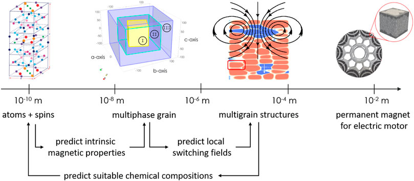
FIGURE 1. Schematics of the lengthscales covered and machine-learning steps used for the design of permanent magnets presented in this paper.

The vision of the approach presented is to provide a toolchain which either guides towards the design of a superior Nd-Fe-B magnet needing less HREEs or which guides towards chemical compositions giving a magnet with adequate magnetic properties for the application but at prices independent of price fluctuations of the REE market. This requires the selection of chemical compositions, the tuning of structural properties and the choice of proper material combinations at the macroscale. Estimated In order to achieve such a bold vision, we have to break up the processes into smaller tasks which are following the length scales scope of view from Angstroms to microns. We try to answer the following questions from the perspective of micromagnetism enhanced by machine learning approaches: i) How are magnetically relevant material properties affected by changes in concentrations of elements in a magnet while focusing on the 2-14-1 phases? ii) What does a single grain inside a large ensemble of grains contribute to coercivity and remanence? iii) How do large ensembles of grains with various grainsizes and secondary phases shape the demagnetization curve? We try to answer these questions from the perspective of micromagnetism enhanced by machine learning approaches.

The paper is organized as follows. In Section 2 the data that were used are described, how it was generated, and how it was incorporated into the models. We further briefly introduce the theoretical background of the applied simulation techniques ranging from first principles simulations to reduced order micromagnetics. We then introduce the machine learning methods applied for building regression models, most importantly partial-least-squares (PLS) regression. We also show how forward machine learning predictors can be combined with genetic algorithms for optimization and inverse design of magnets. Furthermore, we discuss the experimental techniques used for magnetic sample preparation, combinatorial sputtering to produce compostionally graded films, and structural and magnetic characterization. In Section 3 we report the performance of a regression model for the prediction of the spontaneous magnetization and the magneto-crystalline anisotropy constants from the chemical composition of (Nd,Fe,Co,La,Pr)₂(Fe,Co,Ni)₁₄B magnets. We give examples for inverse design of magnetic materials searching for chemical composition required to reach given target values for magnetization and anisotropy. We present the optimal chemical compositions of multi-phase magnets with a core/shell structure with minimum price and maximum coercivity. We also show how machine learning can be used to generate synthetic microstructures that resemble those of sintered magnets and compare the computed demagnetization factors with experimental data. We also analyze the magnetic properties of compositionally graded sputtered films. In Section 4 we discuss the use of machine learning for magnet design. We address open problems and how they might be solved.

2 Materials and methods

2.1 Intrinsic magnetic property prediction

2.1.1 Experimental data foundation

The following described experimental data points are later used to train a machine learning model described in Section 2.1.3 predicting the intrinsic material properties saturation magnetization and magneto-crystalline anisotropy constant. 119 variations of (Nd,Ce,La,Pr)_13.55-(Fe,Co,Ni)_80.54-B_5.91 (at%) alloys were prepared by arc melting. These alloys were annealed at 1373 K for 24 h in Ar atmosphere. After a homogenizing heat treatment, alloy ingots were pulverized and sorted into particles with diameters of $<20\mathrm{\mu }$m in an inert atmosphere to make each particle single crystal.

The powder density was determined using a pycnometer (Ulrtapyc1200e, Quantachrome Instruments, United States). The powder compositions were measured by ICP-AES (ICPS8100, Shimazu, Japan) and the main phase (2-14-1 phase) ratio was calculated from the obtained composition. The magnetic properties were measured by using a vibrating sample magnetometer (PPMS EverCool II, QuantumDesign, United States) at a maximum applied field of 9 T.

Sample powder was mixed with an epoxy resin in a Cu container and solidified in a magnetic field of 1 T for vibrating sample magnetometer (VSM) measurements. M(H) curves of magnetically easy and hard directions were measured in the temperature range from 300 K to 453 K. The magnetic anisotropy field (H_A) was estimated by singular point detection (SPD) method (Cabassi, 2020) from the M(H) curve of hard axis. When anisotropy field is less than 9 T (maximum applied magnetic field of our VSM) H_A can be detected by SPD, otherwise the M(H) curves for both easy and hard axis were extrapolated to higher magnetic field to estimate intersection between them as H_A. On the other hand, saturation magnetization (μ₀M_s) was estimated by the law of approach to saturation (LAS) (Akulov, 1931; Hadjipanayis et al., 1981; Kronmüller et al., 2003) from the M(H) curve of easy axis. When μ₀H_A was lower than the maximum applied field, Eq. 1 was used.

${\mu }_{0}M={\mu }_0{M}_{\mathrm{s}}\left(1-\frac{b}{H^2}\right)(1)$

When μ₀H_A was higher than 9 T, Eqs 2, 3 were used.

${\mu }_{0}M={\mu }_0{M}_{\mathrm{s}}\left(1-\frac{b}{H^2}\right)+{\chi }_{0}H(2)$

${\mu }_0\frac{\mathrm{d}M}{\mathrm{d}H}={\mu }_0{M}_{\mathrm{s}}\left(\frac{2b}{H^3}\right)+{\chi }_0(3)$

M_s is the saturation magnetization and b and χ₀ are constants. The χ₀H term is often referred to as the so-called paramagnetic term (Zhang et al., 2010). Eqs 2, 3 dealing with χ₀ term is more accurate for measuring saturation magnetization, but there is a condition that the applied magnetic field is sufficiently larger than the anisotropy field. The saturation magnetization estimated by the LAS was divided by the main phase ratio of the powder to obtain the saturation magnetization of the 2-14-1 phase in these compositions. For the measurement of the intrinsic properties as described above, grain boundary phases other than the main phase were treated as paramagnetic phases.

2.1.2 First-principles data foundation

The following material database is later used to improve the machine learning model described in Section 2.1.3 predicting the intrinsic material properties saturation magnetization and magneto-crystalline anisotropy constant by appending predicted exchange integral information, Curie temperature and magnetization at 0 K. In this work no attempt to compute the anisotropy constant with first-principles is presented. The material database for the magnetization and Curie temperature (T_C) of ${({\mathrm{N}\mathrm{d}}_{1-\alpha -\beta -\gamma }{\mathrm{Pr}}_{\alpha }{\mathrm{L}\mathrm{a}}_{\beta }{\mathrm{C}\mathrm{e}}_{\gamma })}_2$-${({\mathrm{F}\mathrm{e}}_{1-\delta -\zeta }{\mathrm{C}\mathrm{o}}_{\delta }{\mathrm{N}\mathrm{i}}_{\zeta })}_{14}$-B is constructed using the AkaiKKR program package² (Akai, 1989), where the Korringa-Kohn-Rostoker (KKR) Green’s function method (Korringa, 1947; Kohn and Rostoker, 1954) is implemented within the local density approximation (LDA) of the density functional theory (Hohenberg and Kohn, 1964; Kohn and Sham, 1965). Here, α, β, γ, δ and ζ satisfy the conditions that 0 ≤ α, β, γ, δ, ζ ≤ 1, 0 ≤ α+β+γ ≤ 1 and 0 ≤ δ+ζ ≤ 1. The atomic configurational disorder is treated by the coherent potential approximation (CPA) (Soven, 1970; Shiba, 1971). In the CPA approach, the multiple scattering effects due to random potentials are treated with the single-site approximation. The CPA enables us to calculate the electronic structure and magnetic properties of disordered systems without constructing a large supercell, and hence, is an efficient framework to explore large materials space.

The relativistic effects are included through the scalar relativistic approximation and with spin orbit coupling retaining only the diagonal terms (i.e., l_zs_z terms). LDA, as parametrized by Moruzzi, Janak, and Williams (Moruzzi et al., 2013), is adopted for the exchange-correlation energy functional. The LDA is rather poor for handling strongly localized f states. Therefore, the open core approximation is applied to the f states of the rare earth elements, i.e., Nd, Ce, and Pr, so that the resonances originating from the f states are removed. We assume the electron configurations of Nd³⁺, Ce⁴⁺, and Pr³⁺ in the present calculations.

The T_C is estimated by combining the mean field approximation and the KKR-CPA calculations of magnetic exchange interaction (J_ij) between sites i and j. Here, the Liechtenstein formula (Liechtenstein et al., 1987) is employed to obtain J_ij. According to this formulation, two magnetic atoms are embedded into the CPA effective medium generated by KKR-CPA calculations, and then we evaluate the J_ij values on the basis of the magnetic force theorem, mapping the changes in the band energy due to the infinitesimal rotations of the two magnetic moments to those of the classical Heisenberg Hamiltonian. Experimental lattice parameters are used for R₂T₁₄B (R = Nd, Pr, La, Ce; T = Fe, Co, Ni) when available in literature (Herbst, 1991). Otherwise, the lattice parameters are estimated by integrating first-principles calculation data and available experimental data, as described in Appendix D in (Harashima et al., 2021). The lattice parameters for non-stoichiometric systems are determined from those for stoichiometric systems according to Vegard’s law.

2.1.3 Chemical composition to anisotropy and magnetization with partial least squares

We constructed a model which uses the chemical composition as the only feature to predict the spontaneous magnetization μ₀M_s and the magneto-crystalline anisotropy K₁ of (Nd,La,Ce,Pr)₂(Fe,Co,Ni)₁₄B magnets combining ab-initio data and experimental measurements with partial least-squares regression (PLS). In this section we cover training data preprocessing, analysis and briefly how partial least-squares regression works.

Partial least-squares regression consists of two major parts, i) the decomposition of a matrix into products of smaller matrices similar to principal components analysis (PCA) and ii) the relation between features X and labels Y. In PLS a matrix X is decomposed into a matrix-matrix product of scores T and loadings P such that X = TP^T + E. E here is the residuum. The labels matrix or vector Y is decomposed in the same fashion such that Y = UQ^T + F*. The number of columns in the matrix T is much smaller than the total number of features (the number of columns of the matrix X). Similarly, the matrix U may have much less columns than the number of labels. In other words, both the features and the labels are projected into a latent space. Similar to PCA, the PLS method reduces the dimensionality. Therefore PLS regression is well suited for problems in which either the number of features or the number of labels is large as compared to the number of samples. The scores T are used to predict the Y-scores U. This in turn gives a linear relation between the features and the labels: Y = XB_PLS + B₀. The PLS coefficients B_PLS hold the information of how much each feature contributes to the labels. The latent variables are found through an iterative approach which maximizes the covariance between T and U. In other words the decomposition is built such that i) T best explains the variance in the features, ii) U best explains the variance in the labels, and iii) there is the strongest possible relationship between features and labels (Tobias et al., 1995). There is a lot of well written literature and therefore we may refer to (Geladi and Kowalski, 1986) or (Eriksson et al., 2014) for further reading.

Due to the low amount of training points for heavy rare earth element composites such as with dysprosium (Dy), gadolinium (Gd) and terbium (Tb) it is more difficult to train reliable models and will be covered in future works. These heavy rare earths have been excluded from the training data base as well as entries with holmium (Ho) and manganese (Mn) replacing iron (Fe) and entries where carbon (C) partially replaces boron (B).

Input data for building the machine learning model presented are two data sets: i) Data from ab-initio simulations relating chemical composition to the computed properties such as the spontaneous magnetization, local magnetic moments, the lattice constants, Curie temperature, and the exchange integrals (see Section 2.1.2). ii) Experimental measurements provide the spontaneous magnetization and the anisotropy field for different chemical compositions and temperatures (see Section 2.1.1).

The ab-initio data set and the experimental data do not cover the same combinations of chemical compositions and it is hard to visualize or compute the overlap between two multidimensional sets of partially dependent and independent chemical concentrations of 2-14-1 systems. Our approach is to apply a manifold method exclusively to the ab-initio dataset which transforms each entry to a 2-dimensional projection plane. Each data point receives a repulsive and attractive force between all others, where points close in chemical concentrations attract each other whereas others are pushed away. After relaxation groups of composites will have formed and can be visualized in a 2-dimensional embedding space. In machine learning this is often used to categorize data points in a certain amount of classes, but in our case we use it to gain insight into the overlap of two datasets. After the ab-initio data has been used to calibrate this transformation function, the experimental points are transformed with the same function to verify if those newly added points are far from the ab-initio entries. The result of such a Uniform Manifold Approximation & Projection (UMAP) (McInnes et al., 2018) is shown in Figure 2. One can see that an overlap exists within this projection space which is small but sufficiently encapsulates the ab-initio points. The first principals calculations database consists of many simulations where Co or Ni atoms replace Fe.

FIGURE 2

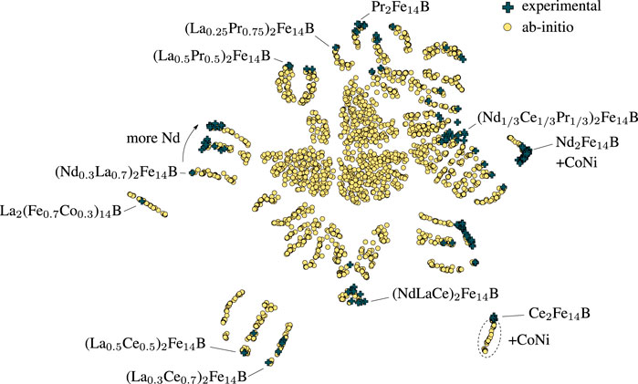
FIGURE 2. UMAP: Two-dimensional embedding space of chemical concentrations from both data sets. Distance between material entries of experimental (blue cross) and first-principles (yellow circle) data. This image illustrates that the overlap between both data sets is small, but experimental points sufficiently encapsulate the ab-initio points.

Using the ab-initio data, we train a first model that predicts ab-initio data from the chemical composition (see i) in Figure 3). We use this partial least squares regressor to augment the experimental data with predicted values for the ab-initio data (see ii) in Figure 3). In addition, we add estimates for M_s(T) and $M_s^3(T)$ estimating the spontaneous magnetization at temperature T with Kuz’min’s equation (Kuz’min, 2005) from the ab-initio-calculated magnetization at 0 K and the Curie temperature. By adding the ab-initio data to the experimental data set, we increase the total number of features which are then used to predict the temperature dependent magnetization and anisotropy with a second partial least squares regressor (see iii) in Figure 3).

FIGURE 3

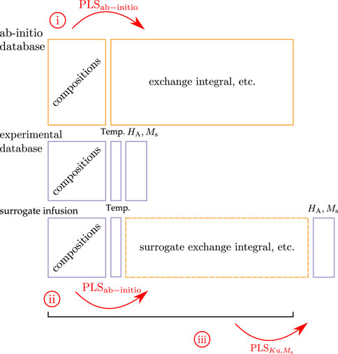
FIGURE 3. Sketch of the 3-step plan to add ab-initio data into the experimental database. (i) Training a PLS regression predicting chemical composition to exchange integral information, (ii) applying this regression model to the experimental database and (iii) training a new PLS model to predict with chemical composition and infused surrogate exchange integral features the intrinsic material properties K₁ and M_s.

To choose the correct number of decomposing components we use nested cross-validation. The data sets shown in Figure 3 are split 5 times into a test set and a training set. With the training set we perform a 5-times repeated 5-fold cross validation. For hyperparameter-optimization we include the polynomial degree of features in the partial least squares regression to leave it to the optimization if higher order contributions should be included or not. The mean squared errors averaged over the test sets are 0.31 MJ/m³ and 0.04 T for K₁ and μ₀M_s, respectively. The feature vector is extended by all combinations of products (2nd degree polynomial) and the final model had 35 components for the partial least squares regression. The forward prediction of this trained model for various chemical compositions is shown in the results section of this manuscript in Section 3.1.

As it is intended to explore and search for new materials, the trained regression is applied to unseen samples of chemical concentration combinations which have no observed or measured output of intrinsic material properties. To gain insight into prediction uncertainty, a rather naive empirical bagging or bootstrapping approach is applied. In our case, not only one but one hundred regressions are calibrated where only slight differences in training data can be found. Each training set is drawn randomly from the full set with the chance of skipping some. The predictions of these hundred regressions provide an average prediction and additionally its prediction variance, referred to as the predictor’s confidence interval (Heskes, 1997). Currently this is our measure of predictor uncertainty but there is potential for improvement here.

Such a trained partial least squares model capable of returning a continuous function of intrinsic material properties along each trained material concentration axis gives an additional opportunity. Combining a multi-objective genetic algorithm framework (Blank and Deb, 2020) with the intrinsic material property predictor can optimize towards a specific target $K_{\mathrm{1}}^{*}$ and $M_{\mathrm{s}}^{*}$ by tuning the chemical concentrations. Similarly, Kim et al. (2018) searched for organic molecules targeting specific molecular designs. Such an inverse design scheme is outlined in Figure 4. There are two objective functions: i) The squared distance between the predicted and the desired K₁ and ii) the squared distance between the predicted and desired μ₀M_s. One major advantage is that we now can define restrictions or constraints to our optimization problem as well e.g., maximum allowed Nd-concentration, only composites of Nd, La and Ce are allowed, and/or the confidence interval has to be below a certain limit.

FIGURE 4

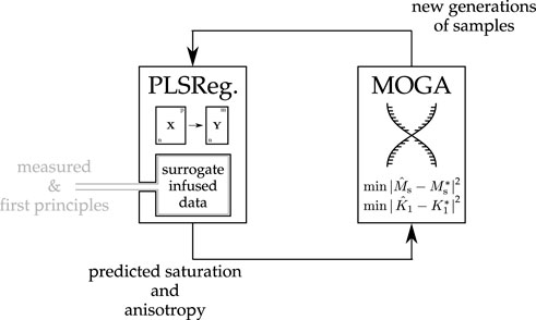
FIGURE 4. Sketch of the inverse design approach, combining the partial least squares regressor, trained with surrogate data, recursively called by a multi-objective optimization genetic algorithm (MOGA) framework, searching for requested intrinsic material properties $K_{\mathrm{1}}^{*}$ and $M_{\mathrm{s}}^{*}$.

2.2 Multi-phase grain coercivity prediction

2.2.1 Automated model generation and micromagnetic simulation

Models of permanent magnets in the range of 10 nm³ to 1 μm³ can be treated with micromagnetic simulations. Micromagnetism is a continuum theory that describes magnetization processes on length scales large enough to replace discrete atomic spins by a continuous function of position M(x) but also small enough to resolve the transition of the magnetization M(x) between magnetic domains. The first argument allows to replace billions of spins with millions of finite elements and hence the computation of demagnetization curves within a reasonable time. The second argument makes it possible to compute the influence of the microstructure on magnetization processes in contrast to macroscopic simulations based on Maxwell’s equations. The key assumption of micromagnetic theory is that the spin orientation changes only by a small angle from one lattice point to the next in a ferromagnet (Brown, 1959). The resolution of the mesh (meshsize) may have significant influence on the energy necessary to form domain walls and the energy required to move domain walls (Donahue and McMichael, 1997). Domain walls might get pinned on too coarse meshes which is an unwanted effect. When simulating permanent magnets, we usually choose a meshsize close to the Bloch wall parameter ${\delta }_0=\sqrt{A/K_1}$ which is a measure of the width of the transition region between two magnetic domains. Exchange constant A and anisotropy constant K₁ of Nd₂Fe₁₄B at room temperature are 8 pJ/M and 4.9 MJ/m³, respectively (Coey, 2010, p. 401). Hence δ₀ = 1.3 nm defines the meshsize close to microstuctural features where the nucleation of reversed domains is likely to happen. While some growth of the meshsize towards the center of the core phase is wanted to speed-up computation, we limited the maximum meshsize to 2δ₀ for unsupervised simulations as it is difficult to automatically detect errors due to artificial pinning of domain walls. This fine discretation limits the maximum modelsize even on today’s computing hardware.

We developed an automated simulation process comprising geometry generation, mesh generation, mesh quality checks, computing the hysteresis properties, and storing the results in a database. The simulation runs completely unsupervised without human interaction. Thus, coercivity data can be sampled in a high-throughput like fashion. The sampler explores the design space and selects a point in feature space. A python script was used to create the multi-phase grain geometry (as sketched in Figure 1) using the open-source software Salome³. MeshGems⁴ was used to create a tetrahedral representation of the geometry. The grains have a brick like shape as shown by transmission electron microscopy (Sepehri-Amin et al., 2013). Such multi-phase grains consist of a core and a shell phase enclosed within a ferromagnetic grain boundary phase. Characteristic features of the core/shell geometry were the thickness of a weakly soft magnetic grain boundary phase (2 nm–50 nm), the thickness of the shell (2 nm–50 nm), the extensions of the grain (60 nm–100 nm in c-direction and 100 nm–150 nm in a- and b-direction), and the misorientation of the grain with respect to the field direction (0°–45°). The hysteresis properties were computed by minimizing the Gibbs free energy considering energy terms due to exchange energy, the magneto-crystalline anisotropy energy, the magnetostatic energy and the Zeeman energy (Exl et al., 2019).

2.2.2 Materials optimization through machine learning

Using micromagnetic simulations we created a database which related chemical composition, grain geometry, and hysteresis properties. We implemented different methodologies to sample the design space. Initially, sample points for training were generated using a Bayesian optimizer (Häse et al., 2018) for maximizing coercivity. In a second stage we applied an active learning scheme. The machine learning predictor for coercivity was used to evaluate the objective function (high coercivity and low Nd + Pr content) of a genetic algorithm. The Pareto points were saved and put into a database for recomputation of the hysteresis properties with the micromagnetic solver. Figure 5 shows the active learning scheme to create additional samples to improve the micromagnetic simulation database.

FIGURE 5

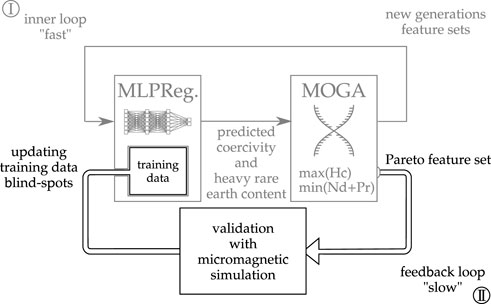
FIGURE 5. Sketch for a proposed active learning scheme which consists of two loops. A fast one (I), in which a multi-objective genetic algorithm tries to find the best solutions–for maximizing the coercivity while minimizing the heavy rare Earth concentration–by testing a shallow neural network. If stopping conditions are met, the second loop is active (II) which receives a set of promising magnet design candidates and validates the prediction by performing a micromagnetic simulation for each. These newly simulated demagnetization curves are then updating the knowledge basis of the shallow neural network.

A neural network regressor is trained to predict the coercive field of multi-phase grains. The model was based on a fully dense neural network as implemented in scikit-learn (Géron, 2019). We used one hidden layer with the number of units as hyperparameter. The rectified linear unit is used as activation function. The mean squared error is used as the loss function which is minimized by the limited-memory Broyden–Fletcher–Goldfarb–Shanno (LBFGS) algorithm (Liu and Nocedal, 1989). The feature vector which contains geometry and intrinsic magnetic properties is augmented with the minimum Stoner-Wohlfarth switching field of the core and shell materials.

In Figure 6 we show the prediction performance as a residual plot and true vs. predicted values for the coercive field of single core-shell grains with defect shells. We included the calibration errors of all micromagnetic simulations as final performance measures: mean absolute error (MAE), root mean squared error (RMSE) and the explained variance (R2). These should not be confused with the predictor performance values during fine tuning of the neural network, which are computed via a 5-fold cross validation. The number of units of the single hidden layer was the only parameter optimized, which gave best results with nine units for the multi-layer perceptron (MLP) regressor inside the sklearn package⁵. The cross validated explained variance is 0.975 and the mean absolute error is 0.148 T.

FIGURE 6

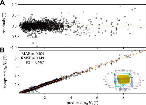
FIGURE 6. (A) prediction residuum over prediction of the coercive field. (B) true micromagnetically computed coercive field over predicted coercive field. Each of those 1908 points refer to a unique micromagnetic multi-phase grain demagnetization simulation, each with different core, shell and grain boundary shape and intrinsic material properties. The inset in the lower right corner shows an example grain structure.

The same bootstrapping approach, as reported in Section 2.1.3, is applied to the coercivity predictor. 100 slightly different training sets are prepared to train 100 neural network regressors, predicting the coercivity. The deviations from their averaged prediction are used to estimate a prediction confidence interval. Additionally all features used for the prediction of coercivity, which depend on the previously predicted material properties are propagated to the prediction uncertainty of coercivity. We think that this is a good measure of the distance in feature space between a point in the test set and the nearest point in the training data.

2.3 Hysteresis of multi-grain structures

2.3.1 Sample preparation and magnetic measurement

Nd-reduced sintered magnets containing Ce and La were fabricated as base sintered magnets. Hydrogen decrepitation and jet-milling processes were used to crush the strip cast flakes into powders. Magnetically aligned green compacts were sintered at 1338 K for 4 h in a vacuum atmosphere. Grain-boundary diffusion was performed at 1223 K for 165 min in vacuum using Nd-Cu based alloys as infiltration materials. This diffusion process forms the core/shell structure in base sintered magnets. The diffused samples were annealed at 773 K for 1 h in vacuum to enhance coercivity.

Magnetic properties were measured by a vibrating sample magnetometer (PPMS EverCool II, QuantumDesign, United States). Scanning electron microscope (SEM) observations were performed using a field emission SEM (ULTRA55, Carl Zeiss, Germany), equipped with an in-lens type detector. SEM observations were performed on specimens milled with an Ar ion beam at an acceleration voltage of 4 kV using an ion milling system (IM4000, Hitachi, Japan) after flat polishing. Crystal structure analysis was carried out by X-ray diffraction (XRD) (SmartLab SE, Rigaku, Japan).

2.3.2 Digital transformation

We apply materials informatics (MI) (Rajan, 2005) to analyze the microstructure of permanent magnets. The following steps were taken to characterize a scanning electron microscope (SEM) image.

1) The two-dimensional power spectrum (Koizumi et al., 2019) obtained by the Fourier transform of the image is converted into a one-dimensional (1D) power spectrum by integrating it in the azimuth direction Figure 7.

2) 10 images of the same magnification per sample are acquired, and the 1D power spectrum converted by the method 1) is averaged.

3) By preparing power spectra of each image and performing principal component analysis of those spectra, the 10 principal components and their weights (principal component scores), the average of all the power spectra, are obtained.

4) The principal component score obtained by 3) is displayed by selecting axes. By coloring each point based on a specific numerical value, for example, it is possible to see whether there is a correlation between the material performance value and the principal component scores.

FIGURE 7

FIGURE 7. (A) SEM image and (B) 2D power spectrum converted from (A). (C) Azimuthal direction integrated 1D power spectrum from (B).

We think that the individualization of analysis and the pre-processing of inhomogeneous data are the bottlenecks in MI, and in order to solve these problems, we have built a common platform for data analysis and storage named “WAVEBASE”⁶. This system is built on a cloud, and users can upload measured data from a web browser. The uploaded data is uniformly pre-processed, features extracted, and visualized in the system. For example, for image analysis, processing is performed by the function 1)-4) above. Data from other techniques such as XRD, small-angle X-ray scattering (SAXS), infrared (IR) and mass spectroscopy can be analyzed in the same way. By utilizing this system, we try to shorten the time from data acquisition to analysis while sharing data and analysis results within multiple joint research institutes.

2.3.3 Synthetic microstructure generation

A power spectrum as shown in Figure 7C characterizes the microstructure of a magnet. We aim to generate synthetic microstructures for micromagnetic simulations that resemble the grain structure of a given magnet. Instead of matching the SEM image with an image derived from the synthetic microstructure we try to create a synthetic microstructure which gives a power spectrum that is similar to that computed from a SEM image. For this purpose, we combine synthetic microstructure generation, neural-network-based image segmentation and a Bayesian optimizer.

We use the software package Neper⁷, which applies Laguerre tessellation for the generation of polycrystalline grains with realistic shape and size distribution (Quey and Renversade, 2018). After slicing the three-dimensional synthetic structure, we create a three-colored image where the different colors represent the main NdFeB phase, the grain boundary phase, and a secondary phase such as for example Nd-oxides. From this artificial microstructure image the power spectrum can be computed. In order to obtain three-colored microstructure images from SEM images we apply automated image segmentation. A convolutional neural network is trained to map a SEM image to a three-color segmented image. We use the well-established unet (Ronneberger et al., 2015; Choudhary et al., 2022) for the network architecture. Instead of manually labeling SEM images we use synthetically generated data for training of the network. Three-colored images which were obtained from synthetic microstructures are randomized by adding noise. Figure 8A shows input output pairs used for training the neural network. Figure 8B shows a SEM image and the segmented three-colored image.

FIGURE 8

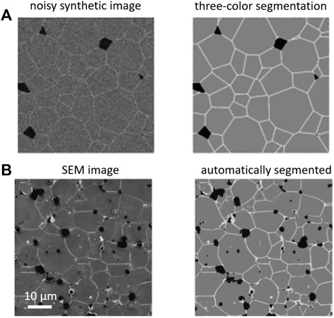
FIGURE 8. (A) Example of an input-output pair for training the neural network for SEM image segmentation. (B) SEM image and its segmentation with the neural network.

The segmentation of the SEM images ensures close similarity in the input color space for the computation of the power spectra between the experimental and the synthetic images. We then apply a Bayesian optimizer⁸ to find a set of input parameters for polycrystalline structure generation with the aim to create a synthetic microstructure which is close to the microstructure of a real magnet. The magnet’s microstructure is characterized by the average of power spectra ${\overline{PSD}}_{\exp }$ obtained from SEM images as described above. To characterize the three-dimensional synthetic grain structure, we compute the average of the power spectra of nine slices through the magnet ${\overline{PSD}}_{\text{syn}}$. The Euclidean norm between the powerspectra $f=|{\overline{PSD}}_{\exp }-{\overline{PSD}}_{\text{syn}}|$ will be minimized during optimization.

2.3.4 Reduced order micromagnetics

For micromagnetic modeling to correctly track magnetic behaviour, various features on multiple length scales have to be taken into account. On the smallest length scale of just a few nanometers crystallographic defects can substantially influence the magnetic reversal of much larger systems. To consider these defects, the model needs to operate on a spatial discretization close to δ₀ in the nanometer regime. Hence, the simulations for large systems require a vast amount of computing resources or are not feasible at all.

To bridge the gap from the nanometer length scale of important microstructural features to a macroscopic length scale, a reduced order model was developed. This model is based on the assumption that nucleation of a sufficiently large reversed domain immediately leads to the magnetic switching of the entire grain in question. Therefore, instead of calculating the state of the magnetic moment on every finite element as in conventional micromagnetism, we assume that each grain is uniformly magnetized and only one macroscopic magnetic moment is assigned per grain. A fast method to approximate the magnetic state of a grain is to employ the embedded Stoner-Wohlfarth (SW) model (Fischbacher et al., 2017; Exl et al., 2018). The embedded approach adapts the original SW method for small ferromagnetic particles to additionally account for long-range interactions of uniformly magnetized grains. Previous research suggests that magnetization reversal of a grain starts close to the edges. Hence, we define evaluation points in all grains at a distance of dL_ex to the grain’s edges. While $L_{\text{ex}}=\sqrt{A/\left({\mu }_0{M}_s^2\right)}$ is the exchange length (Rave et al., 1998), d is a free parameter which will be tuned by comparison to conventional micromagnetics. At these evaluation points the local switching fields are determined analytically by the SW model as

$H_{\text{sw}}=2K_1/\left({\mu }_0{M}_s\right){\left({\sin }^{2/3}\psi +{\cos }^{2/3}\psi \right)}^{-3/2}.$

Here ψ is the angle between the total field acting on the respective point and the magneto-crystalline anisotropy direction of the grain. The total field is the sum of the external field H_ext, the magnetostatic field H_mag and the exchange field H_exch. The magnetostatic field in each point is calculated from the surface charge density by using analytical formulas for polyhedral geometries (Guptasarma and Singh, 1999), employing hierarchical matrices as implemented with h2tools⁹ (Mikhalev and Oseledets, 2016). Hierarchical matrices reduce storage and CPU time, by computing the magnetostatic field from nearby grains exactly, while approximating the field from grains far away from the respective evaluation point. Following the work of Wood, the direction of the magnetization vector of a grain is analytically calculated by the SW model as well (Wood, 2009). This way, in our reduced order model we can also track the reversible part of the demagnetization curve of each grain, and therefore of the entire multigrain system. The exchange field is defined as H_exch = M/l² with l being a phenomenological distance parameter.

We start from a magnetically saturated state with a large positive external field and gradually reverse H_ext in the negative direction until negative saturation. At each field step for each grain we evaluate the total field and check if it overcomes the local switching field H_sw in each point. If multiple grains would switch, only the magnetization of the one with the smallest difference between the total field and H_sw is reversed and the entire system is recomputed. This routine of reversal and recomputation of the total field is done iteratively until a magnetic equilibrium state is reached for the current applied field. Only then this field is reduced by another step and the iterative process starts again.

The free parameters d and l were tuned by comparing calculated coercive fields of single cubic grains to conventional micromagnetic results. We used efficient global optimization (Huang et al., 2006) as implemented in the Dakota suite¹⁰ to find the minimal error for grains with sizes between 100 nm and 800 nm. We included grains with a magneto-crystalline anisotropy direction aligned with the applied field and misaligned by 20°. The intrinsic properties for NdFeB are taken from literature as μ₀M_s = 1.61 T, K₁ = 4.9 MJ/m³ and A = 8 pJ/m. With the optimized parameters d = 1.44 and l = 1.24, the reduced order model can reproduce the coercive fields from conventional micromagnetics very well (see Figure 9).

FIGURE 9

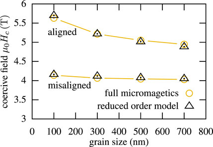
FIGURE 9. Comparison of the reduced order model with classic micromagnetic calculations for single cubic grains of different sizes. The distance parameters for the Stoner Wolfarth evaluation points and exchange field were found by a Bayesian optimizer.

The empirical relation (Kronmüller et al., 1988) for the coercive field

$H_{\mathrm{c}}=\alpha \frac{2K_1}{{\mu }_0{M}_s}-N_{\text{eff}}{M}_{\mathrm{s}}(4)$

is often used to analyze coercivity in permanent magnets. The microstructural parameter α is expected to account for the decrease of the coercive field by soft magnetic defects, misorientation, and intergrain exchange interactions (Kronmüller and Goll, 2002). The microstructural parameter N_eff gives the reduction of the coercive field caused by strong local demagnetizing fields (Grönefeld and Kronmüller, 1989). Experimentally, the microstructural parameters α and N_eff are derived from fitting a straight line to the values of H_c(T)/M_s(T) and $2K_1(T)/({\mu }_0{M}_s^2(T))$ measured at different temperatures T. In micromagnetic simulations, we can compute the microstructural parameters by separating the effects of the demagnetizing field. Computing the demagnetization curve but neglecting the magnetostatic energy term gives $H_{\mathrm{c}}^{*}=\alpha 2K_1/({\mu }_0{M}_s)$ and we can derive $\alpha =H_{\mathrm{c}}^{*}{\mu }_0{M}_s/(2K_1)$. Computing the demagnetizing curve using magnetostatics gives $H_{\mathrm{c}}=H_{\mathrm{c}}^{*}-N_{\text{eff}}{M}_{\mathrm{s}}$. From the difference of the coercive fields computed with and without magnetostatic effects, we obtain the effective demagnetizing factor $N_{\text{eff}}=(H_{\mathrm{c}}^{*}-H_{\mathrm{c}})/M_{\mathrm{s}}$.

2.4 Combinatorial sputtering

A compositionally graded NdCeLaFeB film was fabricated by co-sputtering three targets onto a stationary thermally oxidised Si substrate of diameter 100 mm. The targets were NdFeB, LaFeB, and CeFeB, each with a diameter of 30 mm. The nominal composition of the individual targets (∼RE₁₇Fe_74.5B_8.5) was richer in RE than stoichiometric 2:14:1, to favour the formation of a coercivity inducing RE-rich grain boundary phase. Ta was used as buffer and capping layers, giving the following sample structure: Si/SiO₂/Ta (50 nm)/NdLaCeFeB(1500 nm)/Ta (5 nm). The film was deposited at room temperature and then annealed at 500°C for a duration of 10min, using a rapid thermal annealing furnace (RTA, Jipelec). 2D maps of composition of the as-deposited film were made using Energy Dispersive X-Ray analysis (EDX, Oxford Instruments, spot size $\sim 1\mu$ m) in a scanning electron microscope (SEM, ZEISS). The nominal accuracy of the estimated composition values is of the order of ±1-2 at%. High throughput magnetic characterisation was performed using an in-house developed scanning polar Magneto-Optic Kerr effect (MOKE) system with an integrated coolant-free bi-polar pulsed magnetic field generator and a laser spot size of roughly 50 μm (Dias et al., 2017). The maximum field strength applied at the film surface during a given loop measurement was 4 T. The duration of individual field pulses is of the order of 16 μs, and the delay between positive and negative field pulses is roughly 10 ms. The evolution of crystal structure across the composition gradient was characterized in a high throughput fashion using scanning X-ray diffraction (XRD, Rigaku SmartLab) with Cu-Kα radiation. EDX, MOKE and XRD data points were measured at intervals of 5 × 5 mm². Here XRD was used for high-throughput characterization of the compositionally graded NdCeLaFeB films. For a more detailed characterization of certain new phases characterization methods such as Mössbauer spectroscopy would give additional phase information (Niarchos et al., 2021).

We applied PLS regression in order to predict coercivity from the XRD spectra. PLS regression is well suited for this task, because of its implicit dimensionality reduction. In XRD analysis the number of features, angles at which the scattering intensities were measured, may be higher than the number of samples. Therefore a suitable machine learning method has to be applied when we want to predict material properties such as the coercivity from measured XRD patterns. Indeed, PLS regression has already been widely used in chemistry to analyze spectra (Wold et al., 2001; Eriksson et al., 2014). Machine learning helps to identify important features. In PLS regression a feature is important if the corresponding PLS coefficients are high. Then the feature strongly contributes to Y. On the other hand, a feature is also important if it strongly contributes to the explanation of X given by high loadings which correspond to the feature. The variable importance on projection (VIP) score accounts for both importance on X and Y (Wold et al., 2001). VIP score measures the importance of each feature according to variance explained by each latent variable. The average of the squared VIP scores is one. Therefore features with a VIP score greater than one are considered to be important.

3 Results

3.1 Machine learning of intrinsic magnetic properties

To demonstrate an example of forward model results, predictions of K₁ and μ₀M_s of the trained partial least squares model, over lanthanum concentration with (Nd_x,La_1−x)₂Fe₁₄B are shown in Figure 10 at 300 K and 433 K. The 95% confidence intervals are computed using bootstrapping (Mendez et al., 2020).

FIGURE 10

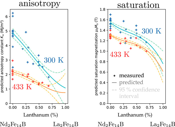
FIGURE 10. Results of trained PLS model to predict with chemical composition and infused surrogate exchange integral features the intrinsic material properties K_u and M_s over lanthanum concentration with (Nd_x,La_1−x)₂Fe₁₄B.

We see that both anisotropy and saturation magnetization decreases with increasing La content. At 433 K the saturation magnetization is close to 1 T if Nd is replaced by 60% La. To make the trained models predictions interpretable, the feature importance can be used. An example is the variable importance on projection (VIP) score of the PLS regression method. A model-agnostic method to compute a feature importance for a prediction has been proposed by Lundberg and Lee (2017) which computes the contributions of a feature by completely removing it from the prediction. Those values are called SHapley Additive exPlanations (in short SHAP values). This can be done globally for a full training data set or locally for one single input feature vector. The major advantage of SHAP values is that they are additive. Starting from the mean model prediction and summing up all important SHAP values gives the final prediction value. In Figure 11 we show a SHAP explanation for the composition (Nd_0.4La_0.6)₂(Fe_0.6Co_0.6)₁₄B at 433 K. We can see that the positive contributions for saturation magnetization result from the increased cobalt content and zero cerium content. The negative contributions are the increased lanthanum concentration and the elevated temperature. The addition of cobalt compensates the loss of saturation magnetization caused by the higher temperature.

FIGURE 11

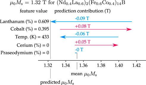
FIGURE 11. SHAP explanation of the prediction of saturation magnetization for (Nd_0.4La_0.6)₂(Fe_0.6Co_0.6)₁₄B at 433 K. SHAP values explain each feature’s positive or negative contribution to the prediction. The sum of all SHAP values and the mean predicted saturation magnetization give the final predicted value. One can see the reduction in M_s caused by the elevated temperature, and that compensation is made with Co.

The above results show that by adding Co it is possible to compensate the loss of M_s owing to La addition. The SHAP plot of Figure 11 shows that increasing the temperature from 300 K to 433 K decreases the saturation magnetization by 0.06 T. In contrast, substituting Sm with a heavy rare-earth such as Gd, Tb or Dy in Sm₂Co₁₇ shows almost zero temperature dependence of remanence in the range from 223 K to 423 K (Hadjipanayis et al., 2006).

3.2 Coercivity of multi-phase grains

In this section, we demonstrate our inverse design approach. Using micromagnetic simulations, we calculated the coercive fields for a platelet-shaped multi-phase grain. The shape and size of the model were inspired by grains found in hot-deformed Nd-Fe-B magnets. A 400 × 400 × 100 nm³ core was enclosed within a 10 nm thick shell. For the simulations we enclosed the multi-phase grain within a 4 nm thick ferromagnetic defect layer (K₁ = 0, μ₀M_s = 1.1 T) which represents the presence of a soft magnetic grain boundary (gb) phase. The volume shares of the core, the shell and the gb are 68%, 22% and 10%, respectively. The intrinsic properties, K₁ and M_s, for the core and shell phase were extracted along a linear fit (dashed line shown in Figure 12) of measured values for chemical compositions at 300 K and do not represent actual measured values. As nucleation is expected to start close to the surface of the multi-phase grain (Grönefeld and Kronmüller, 1989; Fischbacher et al., 2018), K₁ of the shell phase is always higher or equal than K₁ of the core phase. The exchange constant A is assumed to be 8 pJ/m for all three phases. We then reduced K₁ (and consequently M_s) in the core and shell phases until the coercive field μ₀H_c was reduced to 1 T. One suitable phase combination identified was K₁ = 3.77 MJ/m³, μ₀M_s = 1.45 T for the shell phase and K₁ = 0.7 MJ/m³, μ₀M_s = 1.04 T for the core phase. The inverse design approach then predicted (Nd_0.29La_0.36Pr_0.35)₂Fe₁₄B for the shell phase and (La_0.33Ce_0.67)₂(Fe_0.75Co_0.25)₁₄B for the core phase at 300 K. Since this approach can be seen as temperature independent, the same can be done with the 433 K dataset. The predicted chemical compositions are Nd₂(Fe_0.6Co_0.4)₁₄B and (Nd_0.04La_0.22Ce_0.62Pr_0.11)₂(Fe_0.98Co_0.02)₁₄B for shell and core, respectively. The core phase, which represents 68% of the volume, is almost Nd-free. It is recalled that heavy rare Earth elements are not yet included in the predictor.

FIGURE 12

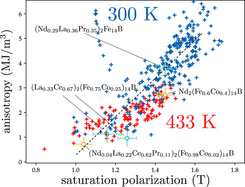
FIGURE 12. Inverse design optimization, by searching for material compositions close to two material property pairs (i) K₁ = 3.77 MJ/m³ and M_s = 1.45 T and (ii) K₁ = 0.7 MJ/m³ and M_s = 1.04 T for different temperatures. Markers show the experimentally acquired pairs at 300 K and 433 K, described in Section 2.1.1. The dashed line is a linear fit through the experimental data at 300 K.

In Figure 12 the bars around the predicted points give the 95% confidence interval of the forward regressor which was evaluated at the best point found by the genetic optimizer. We see that the model uncertainty given by the width of the confidence interval increases with the distance from the experimental data points which are blue crosses for T = 300 K and red crosses for T = 433 K.

With a trained model that predicts coercivities from multi-phase grain geometries and chemical compositions of its phases (explained in Section 2.2.2), we can do inverse modelling: We can search for multi-phase grain structures targeted for a defined coercive field. During optimization we can define conditions, such as only grains with a fixed defect layer thickness or a given maximum Nd content.

Figure 13 demonstrates the two optimization problems and their final Pareto frontiers after 200 generations with a population size of 200. A pareto front is a hypothetical border described by the points of evaluations from an iterative optimization which most efficiently minimize both objective functions. No other points can be found outperforming one objective without losing on the other objective. The two objective functions for both scenarios are maximizing coercivity while minimizing the cost. In both cases the only available material is (Nd_x (Ce_3/4La_1/4)_1−x)₂Fe₁₄B following a press release of Toyota Motor Corporation in 2018¹¹ in which this special lanthanum to cerium ratio has been announced. The difference between the two optimization problems is that in i) a fixed defect shell of 5 nm in each direction has been set which inherits a saturation magnetization 0.8 times the saturation magnetization of the selected shell phase, reflecting some kind of diffusion process. In the second scenario ii) the defect thickness is a free parameter. One can see that the optimization problem for grains with a fixed 5 nm defect reach only 1 T coercivity and cannot be increased anymore by increasing the amount of Nd in the shell phase. On the other hand, if the defect layer thickness is a free parameter, the final population of the optimization consists mainly of designs with the thinnest possible defect, allowing a clear improvement in price efficiency and effective usage of shell Nd in order to increase coercivity.

FIGURE 13

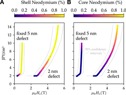
FIGURE 13. Two Pareto frontiers of two inverse design optimizations denoted as (i) fixed 5 nm defect and (ii) 2 nm defect. In both cases the objective was to minimize the cost in JPY/cm³ while maximizing the coercive field. Only (Nd_x (Ce_3/4La_1/4)_1−x)₂Fe₁₄B composites for shell and core materials were allowed. (A) The Pareto set colored with shell Nd (%) and (B) with the core Nd (%). The gray dashed lines show the predictors 95% confidence interval.

3.3 Simulations of hysteresis of multigrain structures

We generated synthetic microstructures of NdFeB magnets by Laguerre tessellation and Bayesian optimization which matches the power spectra of SEM images with those obtained from the synthetic structure. Applying the methodology outlined in Section 2.3.3, we obtained the polycrystalline structure shown in Figure 14. One out of eight experimental SEM images of the magnet whose structure was reconstructed is shown in Figure 8B. The structure generation algorithm minimized the difference between the average power spectrum of the eight experimental images and the average power spectrum of nine slices through the synthetic microstructure. An average grain size of 6.68 μm was obtained for the main phase.

FIGURE 14

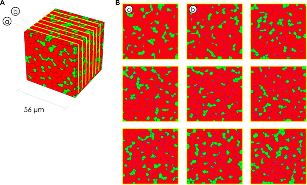
FIGURE 14. Synthetic microstructure generated according to SEM images of sintered NdFeB magnets by matching experimental and synthetically computed power spectra. (A): Three-dimensional grain structure. (B): Nine slices through the structure. The grains of the main phase are red. Non-magnetic inclusions (Nd-Oxides) are green. The grain boundaries shown in black are assumed to be non-magnetic. The structure is generated to resemble that of a magnet with the SEM image shown in Figure 8B.

The newly developed reduced order model based on the embedded Stoner-Wohlfarth model enables the fast computation of demagnetization curves of large multigrain systems. To validate our new model we compare computed demagnetization curves of a cube to the results of conventional micromagnetics. The cube has 160 grains with a mean grain size of 0.1 μm (see inset in Figure 16A). The grains are decoupled by a non-magnetic boundary phase. The intrinsic properties for Nd₂Fe₁₄B are taken from literature as μ₀M_s = 1.61 T, K₁ = 4.9 MJ/m³ and A = 8 pJ/m. On average, each grain has about 2000 points where the local switching field is evaluated. The magneto-crystalline anisotropy direction assigned to the grains is uniformly distributed with a maximal deviation of 35° from H_ext. The resulting demagnetization curves in Figure 15 show very good agreement along the entire reversal process. Along the curves the reversed grains are shown at three different field values. For both models the reversal of the system starts with the same grain. While individual grains deviate, most of the demagnetization progresses via the same grains.

FIGURE 15

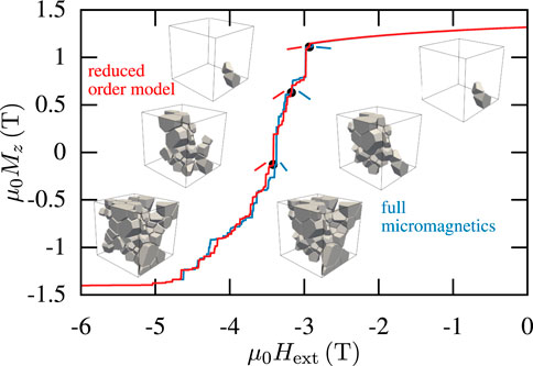
FIGURE 15. Comparison of the demagnetization curve calculated by the reduced order model (red) and the curve calculated by conventional micromagnetics (blue). The insets show the portion of switched grains at three different values of the external field for both models.

Encouraged by this promising result, we enlarged the system to length scales inaccessible by conventional micromagnetic models. We calculate the demagnetization curves of cubes with 160 grains for five different grain sizes from 0.1 μm to 29.3 μm. The cube with the biggest grains has an edge length of 128 μm. For each cube with a specific grain size we generate ten variations of the granular structure to calculate an average demagnetization curve. In Figure 16A the curves of these variations are plotted in light colors, while the darker lines of the respective colors represent their average. The inset shows an example of the used microstructure. With increasing grain size the slope of the demagnetization curve increases and the coercive field decreases. This can be solely attributed to the increased magnetostatic field of larger grains. Furthermore, the distribution of H_c broadens with increasing grain size.

FIGURE 16

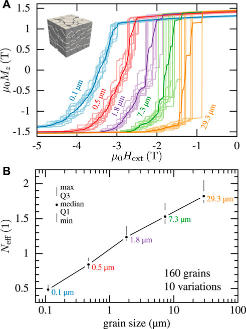
FIGURE 16. (A) Demagnetization curves for cubes with 160 grains of different average grain size. The dark colored curves are the average of curves of ten structure variations drawn in the brighter version of the same color. (B) Calculated local effective demagnetization factor N_eff depending on the grain size of the cube. The depicted distribution for each grain size is calculated from ten microstructural variations. The circles mark the median; the gray lines show the distance between minimum and first quartile (Q1) and maximum and third quartile (Q3), respectively.

Figure 16B shows the calculated demagnetization factor N_eff for a synthetic microstructure consisting of 160 grains as function of grain size. In this simulation the grains were decoupled with a non-magnetic grainboundary phase. The demagnetizing factor increases with increasing grain size. The microstructural parameter resulting from the misorientation of the grains is α = 0.55. The results of the reduced order model are consistent with both experiments and previous mircomagnetic results for a single grain (Bance et al., 2014). Here we compare the computed demagnetizing factors with those of commercial sintered NdFeB magnets. Depending on the heat treatment the demagnetizing factor ranges from 1.0 to 1.5. The grain size distribution for the sintered magnet is shown in Figure 17. In order to obtain the grain size distribution we used four SEM images, we manually labeled the grain boundaries and derived the surface area of the grains with the image processing tool ImageJ (Schneider et al., 2012). The resulting grain size distribution from 2D images was corrected using the method of Saltykov (Saltykov, 1961). For this purpose we applied the software GrainSizeTools (Lopez-Sanchez, 2018). The average grain size is 6.42 μm which is close to the value 6.68 μm obtained by matching the experimental and synthetically computed power spectra. The resulting microsctructure is shown in Figure 14.

FIGURE 17

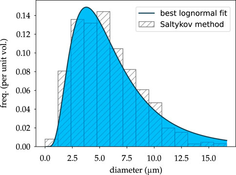
FIGURE 17. Obtained grain size distribution of four SEM images. After manual labeling of grain boundaries the surface areas of the grains were derived with the image processing tool ImageJ (Schneider et al., 2012) and corrected with the method of Saltykov (1961) using GrainSizeTools (Lopez-Sanchez, 2018).

3.4 High throughput methods, combinatorial sputtering

EDX composition maps of the as-deposited NdCeLaFeB film are shown in Figure 18A. Note that only the rare earth (RE) and Fe content is considered (i.e., B is neglected). The RE gradients respect the relative disposition of the individual targets, with the Nd, Ce and La contents being highest in the south-west, east and north-west, respectively. Despite the composition of the individual targets being very close, the Fe content varies somewhat, from a maximum value close to 86 at% to a minimum close to 80 at%. The higher maximum content of Ce compared to Nd and La is tentatively attributed to an inhomogeneity in the sputtering plasma. A 2D array of MOKE loops and the corresponding coercivity map of the annealed NdCeLaFeB film is shown in Figures 18B,C. Coercivity is found to vary across the wafer, with the highest values found in the south of the wafer, where the content of La is lowest. Comparing spatial variations in EDX and MOKE data allows us to plot coercivity on a ternary diagram of Ce, La and Nd content as a percentage of total rare earth (TRE) content (Figure 18D). The zone of maximum coercivity is limited to low La content ($<12.5$%), and stretches to a Ce content of close to 60%. The drop in coercivity with increasing Nd content identified with a red dashed line in the ternary coercivity diagram is attributed to the drop in TRE content in this region of the ternary diagram (Figure 18E).

FIGURE 18

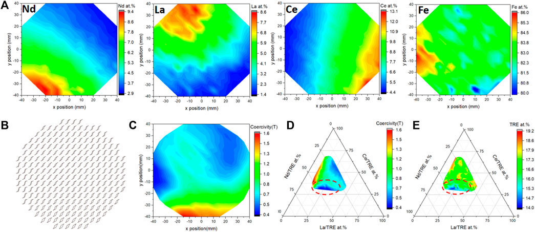
FIGURE 18. (A) EDX maps of Nd, La, Ce and Fe content of a NdCeLaFeB film deposited at room temperature, (B) MOKE loops and (C) coercivity map, (D) coercivity and (E) total rare earth as a function of rare earth over total rare earth content of a NdCeLaFeB film annealed at 500°C for 10 min.

High throughput XRD analysis was applied over an area of 60 by 80 mm². Examples of XRD waterfall plots measured along specific lines are shown in Figure 19. The diffraction peak positions from the powder diffraction file (PDF) card of Nd₂Fe₁₄B (ICSD 00-036-1296) is overlaid on the lower x-axis of both patterns for reference, and all observed XRD peaks can be assigned to the 2-14-1 structure. The diffraction peak positions from the PDF card of Ce₂Fe₁₄B (ICSD 01-079-9727) are overlaid on the upper x-axis of Figure 19A, as the measured points stretch towards Ce-rich compositions while those of La₂Fe₁₄B (ICSD 01-079-9726) are overlaid on the upper x-axis of Figure 19B, as the measured points stretch towards La-rich compositions. Comparison of the experimental peak positions with the PDF cards suggests that La has a lower tendency than Nd and Ce to enter the 2-14-1 crystal structure.

FIGURE 19

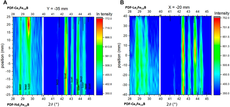
FIGURE 19. XRD waterfall map along lines (A) y = −35 mm and (B) x = −20 mm of the NdCeLaFeB film.

From the data which is shown in Figures 18, 19 we know the local chemical composition, local XRD pattern, and the locally measured coercive field. Machine learning can be used to create a regression model that predicts the coercive field from the chemical composition and the XRD pattern. The features are the XRD intensities sampled for 2ϑ ranging from 28° to 31° and from 40.5° to 45.5° with a step size of 0.04° and the chemical composition Nd, La, Ce, Fe. This gives a total number of 206 features. The total number of samples, positions at which data is available, is 209. PLS regression is a suitable method for a problem for which the number of features is approxmately the same as the number of samples. Therefore, we applied PLS regression to predict the coercive field from the local XRD pattern and the local chemical composition.

We split the total available data randomly into a test and a training set. For the test set we randomly picked 20% to be used for testing the final machine learning model. The remaining 80% of the data were used for training. First, we applied 5-fold cross validation to determine the best number of PLS components. A maximum average R² score was achieved with seven PLS components. Figure 20A shows the measured versus predicted values for the coercive field. The mean absolute error and the R² score for the test set are 0.09 T and 0.81, respectively. Figure 20B gives the 95% confidence interval at the different points on the wafer. The confidence interval was computed using bagging (Mendez et al., 2020). For most points the size of the confidence interval is in the range from 0.1T to 0.15 T. Figures 20C, D give the variable importance on projection (VIP) and the PLS coefficient for the XRD peaks and the chemical elements, respectively. A VIP score greater than 1 is important for the coercive field. Comparing the VIP scores $>1$ and the peak positions from the PDF cards of the pure RE₂Fe₁₄B phases which are well resolved (i.e., the peaks between 41° and 42.5°) shows that the PLS regression identifies peaks with lattice parameters between those of Nd₂Fe₁₄B and Ce₂Fe₁₄B as important contributions to the coercive field. The positive peak in the PLS coefficient at around 30.2° corresponds to a VIP score $>1$. This peak contributes positively to the coercive field and it is tentatively attributed to a RE-rich phase (Ren et al., 2018). The VIP peak at 29.13° may indicate a peak of pure La (ICSD 04-001-0368). The corresponding PLS coefficient is negative. The contributions of the different elements to the coercive field are clearly seen in Figure 20D. All VIP scores are $>1$. The most important variable is the Nd content with a VIP score reaching almost 3. Nd has positive effect on the coercivity with a high positive PLS coefficient. Ce and La both have a negative effect on the coercivity. La reduces the coercivity greater than Ce. The PLS coefficient of Fe is negative. Increasing the Fe content reduces the coercive field because the total RE content is decreasing.

FIGURE 20

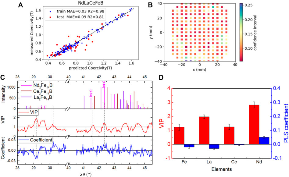
FIGURE 20. (A) Measured coercivity versus coercivity predicted from the XRD pattern and chemical composition, (B) 95% confidence interval for the coercivity prediction of different points on the wafer, (C) peaks of the PDF cards of the pure RE₂Fe₁₄B phases, variable importance on projection (VIP) and PLS coefficient for the XRD peak positions, and (D) VIP and PLS coefficient for the different chemical elements.

4 Discussion

Machine learning assisted materials design may lead to tailored magnetic materials. However, in materials science the available data to establish reliable machine predictions is limited. Accurate physics simulations based on electronic structure and micromagnetic theory are time consuming even on modern hardware. Similarly, gathering experimental data, which relates structure and property of magnetic materials is cumbersome. In this work we proposed different strategies to address these problems. i) The combination of experimental data sets and data obtained from physics simulation may lead to reliable machine learning models. ii) High-throughput measurements on sputtered magnetic films are a means to generate data quickly and in an automated fashion.

To judge the quality of the predictions, the explained variance and the model uncertainty need to be tracked. Though standard statistical methods are available for these tasks, further improvement of the methodologies to test the robustness of regression models and to quantify model uncertainties are needed. Simulated data as input for machine learning models may create a biased model. For intrinsic magnetic data, fusion as presented previously by (Harashima et al., 2021) helps to reduce the error introduced by the approximations of the simulations. On the other hand, the predictor performance for estimating intrinsic magnetic properties can be improved when the experimental datasets are augmented with ab initio data as shown in Section 2.1.3. At the mesoscopic length scale, at which grain morphology, secondary phases, and grain boundary phases are relevant, building of synthetic microstructures that resemble real magnets is a prerequisite for the critical assessment of simulation results. To address this problem we developed methodologies for grain structure generation based on experimental data and micromagnetic simulations for large-grained magnets.

A possibility for the critical review of machine learning models is the comparison of model interpretation results with the well-established expert knowledge in the field. Additive variable importance, as provided by SHAP values, quantitatively explains how the various chemical elements contribute to the intrinsic magnetic properties of magnetic materials. Similarly, the variable importance on projection (VIP) identifies the important peaks in the XRD pattern, the associated phases of which have a strong impact on the coercive field of permanent magnets.

Table 1 shows the applied machine learning models, their input features, predicted outputs and their explained variance measure R².

TABLE 1

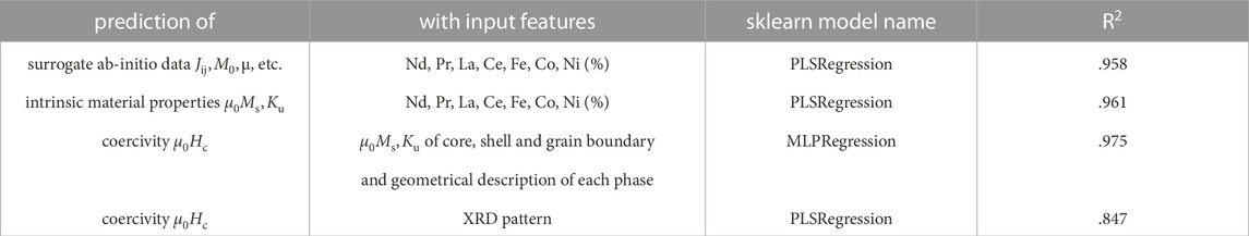
TABLE 1. Summary of applied machine learning models described in Sections 2.1 and 2.2. All R² values have been computed with the full data set but through 5-fold cross-validation. R² is the percentage of how much variance of the predicted quantity can be explained by the trained model.

We demonstrated the possibility of inverse design of magnetic materials. Starting from the desired spontaneous magnetization and magneto-crystalline anisotropy, we estimated possible chemical compositions with intrinsic magnetic properties close to the target values. Furthermore, we can search for Nd-lean magnets composed of core/shell grains with a low price and high coercive field. These magnets are typically fabricated by diffusion of Nd along the grain boundaries in a base magnet with low or zero Nd content (Sepehri-Amin et al., 2013; Ito et al., 2016). Restricting the search space to a base material in which the Ce to La ratio is 3:1, we show that a coercive field close to 1 T can be reached with a Nd-free core under the assumption of unavoidable soft defects with a thickness of 5 nm. This result was obtained using micromagnetic simulations of single multi-phase grains which is a crude approximation. Once generative models for multi-phase multi-granular structures that resemble the microstructure of real magnets are fully established, it will be possible to apply inverse design for the joint optimization of the chemical composition and the magnet’s grain structure. Advances in high-throughput experimental measurements will contribute to overcome this challenge. One example is systematic microstructure variation in terms of grain size or secondary phase of sputtered thin films and the proper local measurement of the grain size by scanning SEM or XRD analysis.

In this work, we adopted feature extraction within a magnetic material data set obtained from a systematically designed experimental data space. In our case, good features from XRD spectra could be extracted by dimensionality reduction for modeling performance of materials by machine learning. We also apply this method to other materials, e.g. catalyst, battery, and carbon materials, and in each case the extracted feature appears to be suitable for expressing their objective value, performance, porosity, etc. In the future, by introducing the WAVEBASE system, it will be possible for collaborators to always share the latest data and analysis results in real time, and we will assess whether it will lead to the acceleration of research.

Data availability statement

The datasets presented in this article are not readily available because the experimental, ab-initio and micromagnetic datasets will not be available in a repository but can be provided after concluding agreement if requested at the corresponding author. Requests to access the datasets should be directed to TSh, thomas.schrefl@donau-uni.ac.at.

Author contributions

TSh, AKt, ND, HA, TM, and TSc contributed to conception and design of the study. AKv, JF, HO, YH, AKr, QA, MG, TF, and NK performend simulations and machine learning analysis. AKn, SG, TD, NS, and YH performed experiments and measurements. MY and AKv organized the data. AKv and JF wrote the first draft of the manuscript. AKv, JF, HO, NS, YH, TF, and TSc wrote sections of the manuscript. All authors contributed to manuscript revision, read, and approved the submitted version.

Funding

The work was partly carried out within the framework of the “Christian Doppler Laboratory for magnet design through physics informed machine learning” funded by the Christian Doppler Research Association. This work was supported by MEXT as “Program for Promoting Researches on the Supercomputer Fugaku” (DPMSD, Grant ID: JPMXP1020200307). The LANEF framework (No. ANR-10-LABX-51-01) is acknowledged for its support with mutualized infrastructure. Institut NEEL received funding from the Toyota Motor Corporation.

Acknowledgments

The financial support by the Austrian Federal Ministry for Digital and Economic Affairs, the National Foundation for Research, Technology and Development, Austria and the Christian Doppler Research Association, Austria is gratefully acknowledged. Data of first-principles computations used in this work was computed using the facilities of the Supercomputer Center of the Institute for Solid State Physics at the University of Tokyo, and computational resources of supercomputer Fugaku provided by the RIKEN Center for Computational Science (Project ID: hp220175).

Conflict of interest

MY, NS, AKn, TSh, and AKt were employed by Toyota Motor Corporation.

The remaining authors declare that the research was conducted in the absence of any commercial or financial relationships that could be construed as a potential conflict of interest.

Publisher’s note

All claims expressed in this article are solely those of the authors and do not necessarily represent those of their affiliated organizations, or those of the publisher, the editors and the reviewers. Any product that may be evaluated in this article, or claim that may be made by its manufacturer, is not guaranteed or endorsed by the publisher.

Footnotes

¹http://153.97.176.35/magnetpredictor, accessed 24-10-2022.

²http://kkr.issp.u-tokyo.ac.jp, accessed: 17-10-2022.

³https://www.salome-platform.org/, accessed 19-10-2022.

⁴www.meshgems.com, now https://www.spatial.com/products/3d-precise-mesh, accessed 19-10-2022.

⁵https://scikit-learn.org/

⁶https://www.toyota.co.jp/wavebase, accessed 17-10-2022.

⁷https://neper.info/, accessed 24-10-2022.

⁸https://scikit-optimize.github.io/stable/, accessed 24-10-2022.

⁹https://pythonhosted.org/h2tools, accessed 17-10-2022.

¹⁰https://dakota.sandia.gov/, accessed 24-10-2022.

¹¹https://global.toyota/en/newsroom/corporate/21139684.html, accessed 09-11-2022.

References

Akai, H. (1989). Fast Korringa-Kohn-Rostoker coherent potential approximation and its application to FCC Ni-Fe systems. J. Phys. Condens. Matter 1, 8045–8064. doi:10.1088/0953-8984/1/43/006

CrossRef Full Text | Google Scholar

Akulov, N. (1931). Über den Verlauf der Magnetisierungskurve in starken Feldern. Z. für Phys. 69, 822–831. doi:10.1007/bf01339465

CrossRef Full Text | Google Scholar

Bance, S., Seebacher, B., Schrefl, T., Exl, L., Winklhofer, M., Hrkac, G., et al. (2014). Grain-size dependent demagnetizing factors in permanent magnets. J. Appl. Phys. 116, 233903. doi:10.1063/1.4904854

CrossRef Full Text | Google Scholar

Binnemans, K., Jones, P. T., Müller, T., and Yurramendi, L. (2018). Rare earths and the balance problem: How to deal with changing markets? J. Sustain. Metallurgy 4, 126–146. doi:10.1007/s40831-018-0162-8

CrossRef Full Text | Google Scholar

Blank, J., and Deb, K. (2020). Pymoo: Multi-objective optimization in Python. IEEE Access 8, 89497–89509. doi:10.1109/ACCESS.2020.2990567

CrossRef Full Text | Google Scholar

Brown, W. F. (1959). Micromagnetics, domains, and resonance. J. Appl. Phys. 30, S62–S69. doi:10.1063/1.2185970

CrossRef Full Text | Google Scholar

Cabassi, R. (2020). Singular point detection for characterization of polycrystalline permanent magnets. Measurement 160, 107830. doi:10.1016/j.measurement.2020.107830

CrossRef Full Text | Google Scholar

Choudhary, A. K., Jansche, A., Grubesa, T., Trier, F., Goll, D., Bernthaler, T., et al. (2022). Grain size analysis in permanent magnets from kerr microscopy images using machine learning techniques. Mater. Charact. 186, 111790. doi:10.1016/j.matchar.2022.111790

CrossRef Full Text | Google Scholar

Coey, J. M. D. (2010). Magnetism and magnetic materials. Cambridge University Press. doi:10.1017/CBO9780511845000

CrossRef Full Text | Google Scholar

Deetman, S., Pauliuk, S., van Vuuren, D. P., van der Voet, E., and Tukker, A. (2018). Scenarios for demand growth of metals in electricity generation technologies, cars, and electronic appliances. Environ. Sci. Technol. 52, 4950–4959. doi:10.1021/acs.est.7b05549

PubMed Abstract | CrossRef Full Text | Google Scholar

Dengina, E., Bolyachkin, A., Sepehri-Amin, H., and Hono, K. (2022). Machine learning approach for evaluation of nanodefects and magnetic anisotropy in FePt granular films. Scr. Mater. 218, 114797. doi:10.1016/j.scriptamat.2022.114797

CrossRef Full Text | Google Scholar

Dias, A., Gomez, G., Givord, D., Bonfim, M., and Dempsey, N. M. (2017). Preparation and characterisation of compositionally graded SmCo films. AIP Adv. 7, 056227. doi:10.1063/1.4977228

CrossRef Full Text | Google Scholar

Donahue, M., and McMichael, R. (1997). Exchange energy representations in computational micromagnetics. Phys. B Condens. MatterHysteresis Model. Micromagnetism 233, 272–278. doi:10.1016/S0921-4526(97)00310-4

CrossRef Full Text | Google Scholar

Eriksson, L., Trygg, J., and Wold, S. (2014). A chemometrics toolbox based on projections and latent variables. J. Chemom. 28, 332–346. doi:10.1002/cem.2581

CrossRef Full Text | Google Scholar

European Commission, Directorate-general for internal market, E., industry, SMEs, S. Bobba, S. Carrara, J. Huismanet al. (2020b). Critical raw materials for strategic technologies and sectors in the EU: A foresight study (Luxembourg: Publication office of the European Union). doi:10.2873/58081

CrossRef Full Text | Google Scholar

European Commission, Directorate-general for internal market, E., industry, SMEs, G. Blengini, C. El Latunussa, U. Eynardet al. (2020a). Study on the EU’s list of critical raw materials (2020): Critical raw materials factsheets (Publications Office). doi:10.2873/92480

CrossRef Full Text | Google Scholar

Exl, L., Fischbacher, J., Kovacs, A., Oezelt, H., Gusenbauer, M., and Schrefl, T. (2019). Preconditioned nonlinear conjugate gradient method for micromagnetic energy minimization. Comput. Phys. Commun. 235, 179–186. doi:10.1016/j.cpc.2018.09.004

CrossRef Full Text | Google Scholar

Exl, L., Fischbacher, J., Kovacs, A., Oezelt, H., Gusenbauer, M., Yokota, K., et al. (2018). Magnetic microstructure machine learning analysis. J. Phys. Mater. 2, 014001. doi:10.1088/2515-7639/aaf26d

CrossRef Full Text | Google Scholar

Fischbacher, J., Kovacs, A., Exl, L., Kühnel, J., Mehofer, E., Sepehri-Amin, H., et al. (2017). Searching the weakest link: Demagnetizing fields and magnetization reversal in permanent magnets. Scr. Mater. 154, 253–258. doi:10.1016/j.scriptamat.2017.11.020

CrossRef Full Text | Google Scholar

Fischbacher, J., Kovacs, A., Exl, L., Kühnel, J., Mehofer, E., Sepehri-Amin, H., et al. (2018). Searching the weakest link: Demagnetizing fields and magnetization reversal in permanent magnets. Scr. Mater. 154, 253–258. doi:10.1016/j.scriptamat.2017.11.020

CrossRef Full Text | Google Scholar

Geladi, P., and Kowalski, B. R. (1986). Partial least-squares regression: A tutorial. Anal. Chim. Acta 185, 1–17. doi:10.1016/0003-2670(86)80028-9

CrossRef Full Text | Google Scholar

Géron, A. (2019). Hands-on machine learning with Scikit-Learn, Keras, and TensorFlow: Concepts, tools, and techniques to build intelligent systems. Sebastopol: O’Reilly Media, Inc.

Google Scholar

Grönefeld, M., and Kronmüller, H. (1989). Calculation of strayfields near grain edges in permanent magnet material. J. Magnetism Magnetic Mater. 80, 223–228. doi:10.1016/0304-8853(89)90122-4

CrossRef Full Text | Google Scholar

Guptasarma, D., and Singh, B. (1999). New scheme for computing the magnetic field resulting from a uniformly magnetized arbitrary polyhedron. GEOPHYSICS 64, 70–74. doi:10.1190/1.1444531

CrossRef Full Text | Google Scholar

Gusenbauer, M., Oezelt, H., Fischbacher, J., Kovacs, A., Zhao, P., Woodcock, T. G., et al. (2020). Extracting local nucleation fields in permanent magnets using machine learning. npj Comput. Mater. 6, 89–10. doi:10.1038/s41524-020-00361-z

CrossRef Full Text | Google Scholar

Hadjipanayis, G. C., fang Liu, J., Gabay, A., and Marinescu, M. (2006). Current status of rare-Earth permanent magnet research in USA. J. Iron Steel Res. Int. 13, 12–22. doi:10.1016/S1006-706X(08)60156-9

CrossRef Full Text | Google Scholar

Hadjipanayis, G., Sellmyer, D. J., and Brandt, B. (1981). Rare-Earth-rich metallic glasses. i. magnetic hysteresis. Phys. Rev. B 23, 3349–3354. doi:10.1103/physrevb.23.3349

CrossRef Full Text | Google Scholar

Harashima, Y., Tamai, K., Doi, S., Matsumoto, M., Akai, H., Kawashima, N., et al. (2021). Data assimilation method for experimental and first-principles data: Finite-temperature magnetization of (Nd, Pr, La, Ce)₂(Fe, Co, Ni)₁₄B. Phys. Rev. Mater. 5, 013806. doi:10.1103/PhysRevMaterials.5.013806

CrossRef Full Text | Google Scholar

Häse, F., Roch, L. M., Kreisbeck, C., and Aspuru-Guzik, A. (2018). Phoenics: A bayesian optimizer for chemistry. ACS Central Sci. 4, 1134–1145. doi:10.1021/acscentsci.8b00307

CrossRef Full Text | Google Scholar

Herbst, J. (1991). R₂Fe₁₄B materials: Intrinsic properties and technological aspects. Rev. Mod. Phys. 63, 819–898. doi:10.1103/revmodphys.63.819

CrossRef Full Text | Google Scholar

Heskes, T. (1997). “Practical confidence and prediction intervals,” in Advances in neural information processing systems 9. Editors M. Mozer, M. Jordan, and T. Petsche (Cambridge: MIT Press), 176–182. doi:10.1142/9789814529020

CrossRef Full Text | Google Scholar

Hirota, K., Nakamura, H., Minowa, T., and Honshima, M. (2006). Coercivity enhancement by the grain boundary diffusion process to Nd–Fe–B sintered magnets. IEEE Trans. Magnetics 42, 2909–2911. doi:10.1109/TMAG.2006.879906

CrossRef Full Text | Google Scholar

Hohenberg, P., and Kohn, W. (1964). Inhomogeneous electron gas. Phys. Rev. 136, B864–B871. doi:10.1103/physrev.136.b864

CrossRef Full Text | Google Scholar

Huang, D., Allen, T. T., Notz, W. I., and Zeng, N. (2006). Global optimization of stochastic black-box systems via sequential kriging meta-models. J. Glob. Optim. 34, 441–466. doi:10.1007/s10898-005-2454-3

CrossRef Full Text | Google Scholar

Ito, M., Yano, M., Sakuma, N., Kishimoto, H., Manabe, A., Shoji, T., et al. (2016). Coercivity enhancement in Ce-Fe-B based magnets by core-shell grain structuring. Aip Adv. 6, 056029. doi:10.1063/1.4945040

CrossRef Full Text | Google Scholar

Jin, J., Ma, T., Zhang, Y., Bai, G., and Yan, M. (2016). Chemically inhomogeneous RE-Fe-B permanent magnets with high figure of merit: Solution to global rare Earth criticality. Sci. Rep. 6, 32200. doi:10.1038/srep32200

PubMed Abstract | CrossRef Full Text | Google Scholar

Kim, K., Kang, S., Yoo, J., Kwon, Y., Nam, Y., Lee, D., et al. (2018). Deep-learning-based inverse design model for intelligent discovery of organic molecules. npj Comput. Mater. 4, 67. doi:10.1038/s41524-018-0128-1

CrossRef Full Text | Google Scholar

Kohn, W., and Rostoker, N. (1954). Solution of the Schrödinger equation in periodic lattices with an application to metallic lithium. Phys. Rev. 94, 1111–1120. doi:10.1103/physrev.94.1111

CrossRef Full Text | Google Scholar

Kohn, W., and Sham, L. J. (1965). Self-consistent equations including exchange and correlation effects. Phys. Rev. 140, A1133–A1138. doi:10.1103/physrev.140.a1133

CrossRef Full Text | Google Scholar

Koizumi, S., Ueda, S., Nishikawa, Y., Terao, T., and Kubo, N. (2019). New attempt to combine scanning electron microscopy and small-angle scattering in reciprocal space. J. Appl. Crystallogr. 52, 783–790. doi:10.1107/S1600576719009208

CrossRef Full Text | Google Scholar

Korringa, J. (1947). On the calculation of the energy of a bloch wave in a metal. Physica 13, 392–400. doi:10.1016/0031-8914(47)90013-x

CrossRef Full Text | Google Scholar

Kronmüller, H., Durst, K.-D., and Sagawa, M. (1988). Analysis of the magnetic hardening mechanism in RE-FeB permanent magnets. J. Magnetism Magnetic Mater. 74, 291–302. doi:10.1016/0304-8853(88)90202-8

CrossRef Full Text | Google Scholar

Kronmüller, H., et al. (2003). Micromagnetism and the microstructure of ferromagnetic solids. Cambridge University Press.

Google Scholar

Kronmüller, H., and Goll, D. (2002). Micromagnetic analysis of nucleation-hardened nanocrystalline PrFeB magnets. Scr. Mater. 47, 551–556. doi:10.1016/s1359-6462(02)00176-8

CrossRef Full Text | Google Scholar

Kuz’min, M. (2005). Shape of temperature dependence of spontaneous magnetization of ferromagnets: Quantitative analysis. Phys. Rev. Lett. 94, 107204. doi:10.1103/physrevlett.94.107204

PubMed Abstract | CrossRef Full Text | Google Scholar

Lambard, G., Sasaki, T., Sodeyama, K., Ohkubo, T., and Hono, K. (2022). Optimization of direct extrusion process for Nd-Fe-B magnets using active learning assisted by machine learning and bayesian optimization. Scr. Mater. 209, 114341. doi:10.1016/j.scriptamat.2021.114341

CrossRef Full Text | Google Scholar

Li, W., Zhao, L., and Liu, Z. (2019). Micromagnetic simulation for the effects of core-shell distributions of RE on the magnetic properties of dual-main-phase Nd-Fe-B based magnets. J. Magnetism Magnetic Mater. 476, 302–310. doi:10.1016/j.jmmm.2018.12.107

CrossRef Full Text | Google Scholar

Liechtenstein, A. I., Katsnelson, M., Antropov, V., and Gubanov, V. (1987). Local spin density functional approach to the theory of exchange interactions in ferromagnetic metals and alloys. J. Magnetism Magnetic Mater. 67, 65–74. doi:10.1016/0304-8853(87)90721-9

CrossRef Full Text | Google Scholar

Liu, D. C., and Nocedal, J. (1989). On the limited memory BFGS method for large scale optimization. Math. Program. 45, 503–528. doi:10.1007/bf01589116

CrossRef Full Text | Google Scholar

Liu, D., Ma, T., Wang, L., Liu, Y., Zhao, T., Hu, F., et al. (2019). Computational analysis of microstructure-coercivity relation in multi-main-phase Nd–Ce–Fe–B magnets. J. Phys. D Appl. Phys. 52, 135002. doi:10.1088/1361-6463/aaff42

CrossRef Full Text | Google Scholar

Lopez-Sanchez, M. A. (2018). GrainSizeTools: A Python script for grain size analysis and paleopiezometry based on grain size. J. Open Source Softw. 3, 863. doi:10.21105/joss.00863

CrossRef Full Text | Google Scholar

Lundberg, S. M., and Lee, S.-I. (2017). A unified approach to interpreting model predictions. Adv. neural Inf. Process. Syst. 30.

Google Scholar

Matsumoto, M., Ito, M., Sakuma, N., Yano, M., Shoji, T., and Akai, H. (2019). Optimal uni-axial ferromagnetism in (La,Ce)₂Fe₁₄B for permanent magnets. doi:10.48550/ARXIV.1901.10119

CrossRef Full Text | Google Scholar

McInnes, L., Healy, J., and Melville, J. (2018). Umap: Uniform manifold approximation and projection for dimension reduction. doi:10.48550/ARXIV.1802.03426

CrossRef Full Text | Google Scholar

Mendez, K. M., Broadhurst, D. I., and Reinke, S. N. (2020). Migrating from partial least squares discriminant analysis to artificial neural networks: A comparison of functionally equivalent visualisation and feature contribution tools using jupyter notebooks. Metabolomics 16, 17. doi:10.1007/s11306-020-1640-0

PubMed Abstract | CrossRef Full Text | Google Scholar

Mikhalev, A. Y., and Oseledets, I. V. (2016). Iterative representing set selection for nested cross approximation. Numer. Linear Algebra Appl. 23, 230–248. doi:10.1002/nla.2021

CrossRef Full Text | Google Scholar

Miyake, T., Harashima, Y., Fukazawa, T., and Akai, H. (2021). Understanding and optimization of hard magnetic compounds from first principles. Sci. Technol. Adv. Mater. 22, 543–556. doi:10.1080/14686996.2021.1935314

PubMed Abstract | CrossRef Full Text | Google Scholar

Möller, J. J., Körner, W., Krugel, G., Urban, D. F., and Elsässer, C. (2018). Compositional optimization of hard-magnetic phases with machine-learning models. Acta Mater. 153, 53–61. doi:10.1016/j.actamat.2018.03.051

CrossRef Full Text | Google Scholar

Moruzzi, V. L., Janak, J. F., and Williams, A. R. (2013). Calculated electronic properties of metals. Elsevier.

Google Scholar

Nakamura, H. (2018). The current and future status of rare Earth permanent magnets. Scr. Mater. 154, 273–276. doi:10.1016/j.scriptamat.2017.11.010

CrossRef Full Text | Google Scholar

Niarchos, D., Gjoka, M., Schönhöbel, A. M., Aubert, A., Madugundo, R., Garitaonandía, J. J. S., et al. (2021). Intrinsic magnetic properties of (nd1-xsmx)fe11ti. J. Alloys Compd. 864, 158097. doi:10.1016/j.jallcom.2020.158097

CrossRef Full Text | Google Scholar

Quey, R., and Renversade, L. (2018). Optimal polyhedral description of 3D polycrystals: Method and application to statistical and synchrotron X-ray diffraction data. Comput. Methods Appl. Mech. Eng. 330, 308–333. doi:10.1016/j.cma.2017.10.029

CrossRef Full Text | Google Scholar

Rajan, K. (2005). Materials informatics. Mater. Today 8, 38–45. doi:10.1016/s1369-7021(05)71123-8

CrossRef Full Text | Google Scholar

Rave, W., Ramstöck, K., and Hubert, A. (1998). Corners and nucleation in micromagnetics. J. Magnetism Magnetic Mater. 183, 329–333. doi:10.1016/S0304-8853(97)01086-X

CrossRef Full Text | Google Scholar

Ren, H., Abbas, N., Liu, Y., Tang, H., Gui, W., Ding, J., et al. (2018). Magnetic hardening of Nd-Ce-Fe-B films with high Ce concentration. Sci. Rep. 8, 11599–9. doi:10.1038/s41598-018-29907-4

PubMed Abstract | CrossRef Full Text | Google Scholar

Ronneberger, O., Fischer, P., and Brox, T. (2015). in International Conference on Medical image computing and computer-assisted intervention (Springer), 234–241.U-net: Convolutional networks for biomedical image segmentation

CrossRef Full Text | Google Scholar

Sagawa, M., Fujimura, S., Yamamoto, H., Matsuura, Y., and Hiraga, K. (1984). Permanent magnet materials based on the rare Earth-iron-boron tetragonal compounds. IEEE Trans. Magnetics 20, 1584–1589. doi:10.1109/tmag.1984.1063214

CrossRef Full Text | Google Scholar

Saltykov, S. (1961). STEROMETRIC METALLURGY, PART 1 (STEREOMETRICHESKAYA METALLOGRAFIYA). Tech. rep. AIR FORCE SYSTEMS COMMAND WRIGHT-PATTERSON AFB OH FOREIGN TECHNOLOGY DIVISION.

Google Scholar

Schneider, C. A., Rasband, W. S., and Eliceiri, K. W. (2012). NIH image to ImageJ: 25 years of image analysis. Nat. methods 9, 671–675. doi:10.1038/nmeth.2089

PubMed Abstract | CrossRef Full Text | Google Scholar

Sepehri-Amin, H., Ohkubo, T., Nagashima, S., Yano, M., Shoji, T., Kato, A., et al. (2013). High-coercivity ultrafine-grained anisotropic Nd–Fe–B magnets processed by hot deformation and the Nd–Cu grain boundary diffusion process. Acta Mater. 61, 6622–6634. doi:10.1016/j.actamat.2013.07.049

CrossRef Full Text | Google Scholar

Shiba, H. (1971). A reformulation of the coherent potential approximation and its applications. Prog. Theor. Phys. 46, 77–94. doi:10.1143/ptp.46.77

CrossRef Full Text | Google Scholar

Soven, P. (1970). Application of the coherent potential approximation to a system of muffin-tin potentials. Phys. Rev. B 2, 4715–4722. doi:10.1103/physrevb.2.4715

CrossRef Full Text | Google Scholar

Strnat, K., Hoffer, G., Olson, J., Ostertag, W., and Becker, J. (1967). A family of new cobalt-base permanent magnet materials. J. Appl. Phys. 38, 1001–1002. doi:10.1063/1.1709459

CrossRef Full Text | Google Scholar

Tobias, R. D., et al. (1995). “An introduction to partial least squares regression,” in Proceedings of the twentieth annual SAS users group international conference (Cary, NC, USA): SAS Institute Inc.), 1250–1257.

Google Scholar

Une, Y., and Sagawa, M. (2012). Enhancement of coercivity of Nd-Fe-B sintered magnets by grain size reduction. J. Jpn. Inst. Metals 76, 12–16. doi:10.2320/jinstmet.76.12

CrossRef Full Text | Google Scholar

Wang, Y., Tian, Y., Kirk, T., Laris, O., Ross, J. H., Noebe, R. D., et al. (2020). Accelerated design of Fe-based soft magnetic materials using machine learning and stochastic optimization. Acta Mater. 194, 144–155. doi:10.1016/j.actamat.2020.05.006

CrossRef Full Text | Google Scholar

Wold, S., Sjöström, M., and Eriksson, L. (2001). PLS-Regression: A basic tool of chemometrics. Chemom. intelligent laboratory Syst. 58, 109–130. doi:10.1016/s0169-7439(01)00155-1

CrossRef Full Text | Google Scholar

Wood, R. (2009). Exact solution for a stoner–wohlfarth particle in an applied field and a new approximation for the energy barrier. IEEE Trans. Magnetics 45, 100–103. doi:10.1109/TMAG.2008.2006286

CrossRef Full Text | Google Scholar

Zhang, H., Zeng, D., and Liu, Z. (2010). The law of approach to saturation in ferromagnets originating from the magnetocrystalline anisotropy. J. magnetism magnetic Mater. 322, 2375–2380. doi:10.1016/j.jmmm.2010.02.040

CrossRef Full Text | Google Scholar