Pressure Mapping Using Nanocomposite-Enhanced Foam and Machine Learning

1 Introduction

An ever-increasing number of devices, mainly in healthcare and robotic industries, employ pressure mapping strategies to visualize the contact distribution on its sensing surfaces. For instance, pressure sensing can detect prolonged localized pressures in patients with limited mobility who may develop ulcers due to the difficulty of shifting their weight. Such ulcers can cause tissue necrosis and can lead to death in the most severe cases. Another example is that pressure mapping is largely employed in the automation field to mimic the feeling of touch in sophisticated human-inspired robots. In these applications, high mapping resolution and real-time sensing are of primary importance.

Conventional pressure mapping systems often employ dense grids of discrete transducers or electrodes. In these cases, the mapping resolution is proportional to the density, complexity, and cost of the distributed transducers (Wu et al., 2016; Nela et al., 2018). The need to overcome these limitations, as well as to achieve miniaturization and conformability to complex surfaces, have motivated the development of pressure sensing systems in the form of films (Shirinov and Schomburg, 2008; Nela et al., 2018), textiles (Ryu et al., 2018; Kim et al., 2019), paint (Li et al., 2021), and foams (Wu et al., 2016). Many of these pressure-sensitive materials have been made possible by leveraging the unique material properties of carbon nanotubes (Huang et al., 2017; Nela et al., 2018; Kim et al., 2019; Li et al., 2021), carbon black (Wu et al., 2016), graphene nanosheets (Tao et al., 2017), and conductive polymers (Shirinov and Schomburg, 2008; Ding et al., 2018), among many others (Zang et al., 2015).

Recently, several studies have demonstrated the efficacy of electrical impedance tomography (EIT) and electrical resistance tomography (ERT) for inferring the conductivity distribution of a surface or a solid using only boundary voltage measurements (Gupta et al., 2017; Duan et al., 2019; Tallman and Smyl, 2020; Li et al., 2021; Lin et al., 2021). For this reason, one of the first applications of EIT has been for noninvasive medical imaging, such as for assessing regional lung aeration (Frerichs et al., 2017). On the other hand, recent studies in the mechanical and civil engineering fields have shown how EIT can be effectively employed to detect material discontinuities and strain states that alter the original conductivity of the inspected material (Loh et al., 2009). Because conductivity is pre-calibrated to applied strains, the resulting conductivity distribution of piezoresistive materials can be used to directly visualize the magnitudes and locations of strain concentrations or distributions of strain. In this context, several fabric-based devices were proposed for pressure sensing (Yao and Soleimani, 2012; Duan et al., 2019; Lee et al., 2021; Lin et al., 2021). For instance, Yao and Soleimani (2012) presented a knitted fabric whose conductivity increases with applied pressure. EIT conductivity mapping was employed to identify pressure distributions. Wang et al. (2016) proposed a nanocomposite sensitive fabric. Specifically, a piezoresistive multi-walled carbon nanotube-latex thin film was integrated with flexible fabric. The identification of pressure hotspots was confirmed, and the sensing performance of this device was found to be stable even after handwashing. More recently, Dai and Thostenson (2019) used EIT to map pressure distributions on a relatively large sensing device made of a nonwoven elastomeric composite coated with carbon nanotubes. Out-of-plane loads induced in-plane Poisson expansion of the coated sensing material and showed acceptable resolution performance. Liu et al. (2021) employed a flexible hydrogel-based sensor to reconstruct high-resolution pressure maps. Although some of these materials can be easily produced in laboratories, the dimensions of the sensing area must be known during the fabrication process. As a consequence, these sensing devices are case-specific, and different applications require custom fabrication.

Since the inverse problem in EIT typically involves least squares-based methods, these conventional algorithms may be unsuitable for real-time pressure mapping due to the extensive computational runtime of matrix inversion operations. Moreover, the low resolution of reconstructed images is a well-known issue related to the regularization strategies typically employed by these EIT methods. Instead, machine learning (ML)-based techniques have been applied to solve the strongly nonlinear EIT problem, mainly in the medical field. Duan et al. (2019) applied machine learning to correct the pressure distribution of fabric using the spatiotemporal total variation algorithm and confirmed near-real-time pressure mapping. Lin et al. (2020) showed that an end-to-end artificial neural network (ANN) approach is faster and generally provides more accurate results with respect to hybrid procedures that employ ML to solve parts of the traditional algorithms, although being less general. Radial basis function networks (RBFNs) have demonstrated excellent generalization capabilities and require a small computational footprint to operate, which has thus become particularly suitable for mobile sensing applications. In addition, Wang et al. (2021) has also shown the superior robustness of RBFNs to noise. Husain et al. (2021) recently proposed a tactile sensing solution employing an RBFN followed by segmentation techniques for object recognition. However, end-to-end solutions based on RBFNs that exploit their low computational cost are still rarely used due to the typical low resolution of the outcome.

This study aims to build on the rich body of work in ML-based EIT methods and to compare the spatial conductivity mapping performance of end-to-end RBFN and deep ANN versus the “traditional” total variation method (TV) (Holder, 2004). In particular, the focus is on reconstructing the strain distribution of a smart foam for pressure hotspot monitoring applications. A pressure-sensitive smart foam was prepared by integrating a piezoresistive carbon nanotube-based thin film with a commercially available foam. Different from other sensing devices, in this case, the sensing film is obtained simply by spray-coating the substrate with an airbrush. This solution is thus easily scalable, since the area and shape of the sensing region only depend on the geometry of the substrate.

Pressure sensing tests were performed, while EIT boundary voltage measurements were acquired for different scenarios. The same datasets were used and processed by the RBFN, ANN, and TV-based algorithms to obtain the corresponding conductivity maps for comparison. For the ML-based approaches, a data normalization strategy and noise-assisted regularization process were proposed to obtain robust and accurate conductivity reconstruction.

2 Electrical Impedance Tomography Background

EIT is a soft-field imaging method that uses applied electrical excitations and measurements obtained along the boundaries of a conductive body to estimate its distribution of electrical properties. In short, EIT consists of the forward and inverse problems. The former involves calculating the voltage distribution on the boundary of the interrogated body when the boundary electrical excitation and the spatial conductivity properties of the body itself are known a priori. On the other hand, the inverse problem consists of estimating the conductivity distribution using boundary current excitations and voltage measurements. The EIT inverse problem can be solved when an alternating current excitation is applied and both voltage magnitudes and phases are recorded. In the case of a direct current (DC) excitation, the EIT problem specializes to become electrical resistance tomography (ERT).

2.1 ERT Forward Problem

Let $\text{Ω}$ be a conductive body with conductivity distribution $\sigma$ and boundary $\text{Γ}$. Considering a given number of electrodes deployed along $\text{Γ}$, if DC is injected using at least two of them (a source and a sink), the electric flow in $\text{Ω}$ can be described using Kirchoff’s law, which correlates $\sigma$ with the electric potential distribution $\varphi$ in the absence of any current source or sink inside of $\text{Ω}$:

$\nabla \cdot \sigma \nabla \varphi =0(1)$

Let $\mathbf{n}$ be an outward unit vector normal to $\text{Γ}$, and $j=\sigma \nabla \varphi \cdot \mathbf{n}$ be the current density in $\text{Γ}$. Given $\sigma$, the knowledge of $\varphi$ on the boundary ${\varphi |}_{\text{Γ}}$ (known as Dirichlet boundary condition) is sufficient to uniquely determine $\varphi$. Similarly, knowing $j$ (known as Neumann boundary condition) allows determining $\varphi$ up to an additive constant. An operator that relates Dirichlet and Neumann data can be defined as ${\text{Λ}}_{\sigma }:{\varphi |}_{\text{Γ}}\to j$, which is known as the Dirichlet to Neuman (DtN) map. This operator—or its inverse ${\text{Λ}}_{\sigma }^{-1}$, the Neuman to Dirichlet (NtD) map—represents the response of the system that is electrically interrogated at its boundary.

In this study, electrical current and voltage were applied and measured, respectively, at discrete electrodes, using a finite element (FE) model. In a FE formulation, the region in which the problem is solved is segmented into a finite number of elements. A collection of these elements is herein called “mesh,” and this work employed linear triangular elements. In the FE solution, a weak formulation of the differential Eq. 1 was solved at the mesh nodes using the complete electrode model (CEM) (Holder, 2004). The solution was thus interpolated over each element using shape functions along the edges of the elements. For more details about the FE implementation, the reader can refer to the referenced works (Holder, 2004; Gupta et al., 2017).

2.2 ERT Inverse Problem

The inverse problem, as formulated by Calderón (2006), consists of recovering $\sigma$ from ${\text{Λ}}_{\sigma }$ by injecting currents in a subset of electrodes and measuring the voltage using all the others. Arranging these quantities in vectors (${\mathbf{i}}_q\in {\mathrm{ℝ}}^Q$ and ${\mathbf{v}}_q\in {\mathrm{ℝ}}^Q$, respectively), a discrete equivalent DtN map can be represented in matrix form as:

${\mathbf{i}}_q=\mathbf{Y}{\mathbf{v}}_q(2)$

where $\mathbf{Y}$ represents the transfer admittance matrix (which has real elements in the case of direct current). Different measurement protocols can be applied using predefined interrogation patterns (i.e., given sets of ${\mathbf{i}}_q$ vectors) that allow building a basis for the space of $\mathbf{Y}$. The set of ${\mathbf{i}}_q$ and ${\mathbf{v}}_q$ vectors obtained through interrogation can be employed to reconstruct $\mathbf{Y}$ by inverting Eq. 2. Therefore, the inverse problem in the discrete case becomes recovering a vector $\mathbf{\sigma }\in {\mathrm{ℝ}}^M$ containing the conductivity values of all the $M$ elements of the FE mesh from $\mathbf{Y}$. Alternatively, the inverse problem can be defined in terms of the transfer impedance $\mathbf{Z}={\mathbf{Y}}^{-1}$, which is the discrete counterpart of an inverse operator ${\text{Λ}}_{\sigma }^{-1}:j\to {\varphi |}_{\text{Γ}}$. Also, the inverse problem can be defined for difference imaging, where the variation of conductivity between two different time instances or states (generally, a baseline and an inspection instant) is recovered from a variation in the NtD map. In all these cases, the inverse problem is ill-posed and ill-conditioned (Holder, 2004), which also becomes extremely unstable in the presence of noise.

Several methods have been proposed to solve the inverse problem using a priori information, which mainly consist of regularization criteria (Holder, 2004) that constrain the solution to rule out the variations that cause instability. These methods, which are briefly described in Section 3, generally require the calculation and inversion of a sensitivity matrix that represents the derivative of the voltage measurements with respect to a conductivity parameter. However, complex inversion operations may hinder portable applications where the computational footprint of processing devices is generally limited.

3 Regularization Approaches

Given a current interrogation pattern, consider the matrix of measured boundary voltages $\mathbf{V}=\mathbf{ZI}$, where $\mathbf{V}=\left[{\mathbf{v}}_1,\dots ,{\mathbf{v}}_Q\right]$ and $\mathbf{I}=\left[{\mathbf{i}}_1,\dots ,{\mathbf{i}}_Q\right]$, with the column vectors ${\mathbf{v}}_q$ and ${\mathbf{i}}_q$ defined in Section 2.2. For simplicity of notation, let $\mathbf{v}$ be a vector containing all the elements of $\mathbf{V}$ arranged in a single column.

Considering difference imaging, the voltage measurement used as an input to the inverse EIT problem can be defined as $\text{δ}\mathbf{v}={\mathbf{v}}^{\left(c\right)}-{\mathbf{v}}^{\left(0\right)}$, where ${\mathbf{v}}^{\left(0\right)}$ and ${\mathbf{v}}^{\left(c\right)}$ are the voltage vectors measured in two different states. A similar difference can be defined in the forward problem, as:

$\text{δ}{\mathbf{v}}_{\mathbf{f}}=\mathit{f}\left(\mathbf{\sigma }+\text{δ}\mathbf{\sigma }\right)-\mathit{f}\left(\mathbf{\sigma }\right)(3)$

where $\mathit{f}\left(\mathrm{■}\right)$ is the output of the forward problem evaluated at the conductivity in its argument, and $\text{δ}\mathbf{\sigma }$ is the conductivity change between the two considered states. Truncating the Taylor series expansion of $\mathit{f}\left(\mathbf{\sigma }+\text{δ}\mathbf{\sigma }\right)$ to the first term and defining the sensitivity matrix as the Jacobian $\mathbf{J}=\partial \mathit{f}\left(\mathbf{\sigma }\right)/\partial \mathbf{\sigma }$, an estimate $\text{δ}\widehat{\mathbf{\sigma }}$ of the difference in the conductivity distribution can be calculated by minimizing the difference between $\text{δ}\mathbf{v}$ and $\text{δ}{\mathbf{v}}_{\mathbf{f}}\approx \mathbf{J}\text{δ}\mathbf{\sigma }$, as follows:

$\text{δ}\widehat{\mathbf{\sigma }}=\underset{\text{δ}\mathbf{\sigma }}{\text{arg}\text{min}}(\Vert \mathbf{J}\text{δ}\mathbf{\sigma }-\text{δ}\mathbf{v}{\Vert }^2+\alpha \Vert \mathbf{R}\left(\text{δ}\mathbf{\sigma }\right){\Vert }^2)(4)$

Here, the symbol $\Vert \mathrm{■}\Vert$ denotes the L² vector norm of its argument, $\mathbf{R}\left(\text{δ}\mathbf{\sigma }\right)$ is a regularization matrix, and the scalar parameter $\alpha$ controls its relative contribution. Common regularization approaches are summarized in the referenced work (Tallman and Smyl, 2020). In this study, the TV approach is employed, according to which

$\mathbf{R}\left(\text{δ}\mathbf{\sigma }\right)={\displaystyle \underset{\text{Ω}}{\int }\nabla \text{δ}\mathbf{\sigma }\text{dΩ}}(5)$

and can be practically implemented in an iterative procedure (Holder, 2004).

To date, the L² norm has mainly been used on the error minimization term of Eq. 4 to reduce computational complexity (Tallman and Smyl, 2020). Thereby, it was considered in this study to represent potential portable applications in devices with a small computational footprint. Besides, quadratic regularization functionals have proven particularly effective in reducing oscillations in reconstructed conductivity (Holder, 2004). However, most of these methods typically favor smoothly varying distributions. On the other hand, the total variation functional can also regularize non-smooth profiles, preserving the edges between conductivity artifacts and background conductivity (Holder, 2004; Tallman and Smyl, 2020). Thus, the TV method was used in this work for comparison to reconstruct small and sharp conductivity variations effectively.

4 Machine Learning Approach

In this section, two alternative ML techniques, namely, an artificial deep neural network (DNN) and a radial basis function network (RBFN), were employed to solve the inverse problem. Since supervised learning algorithms were used, specific considerations were necessary for the construction of a training dataset. Herein, the architecture of the ML tools is described, as well as their training process.

4.1 Preparation of the Training Dataset

DNNs and RBFNs have gained considerable interest in the last decades and are currently some of the most popular supervised ML tools used for regression due to their effectiveness in solving nonlinear problems. A training dataset representing examples of input-output pairs must be used to train the ML tools in the preliminary training phase. Then, in the application phase, the trained network can generate an output based only on input data, following the structure learned from the training set.

Let ${\mathbf{v}}^{\left(c\right)}$ and ${\mathbf{\sigma }}^{\left(c\right)}$ be the voltage measurements collected in the selected interrogation pattern and the conductivity distribution of a given ($c$^th) condition of the inspected body, respectively. A normalized difference of voltage measurement and conductivity distribution in configuration $c$ can be defined as:

$\text{δ}{\overline{\mathbf{v}}}^{\left(c\right)}=\frac{{\mathbf{v}}^{\left(c\right)}-{\mathbf{v}}^{\left(0\right)}}{\widehat{v}}(6)$

$\text{δ}{\mathbf{\sigma }}^{\left(c\right)}={\mathbf{\sigma }}^{\left(c\right)}-{\mathbf{\sigma }}^{\left(0\right)}(7)$

where ${\mathbf{v}}^{\left(0\right)}$ and ${\mathbf{\sigma }}^{\left(0\right)}$ represent the boundary voltage at the electrode locations and the conductivity values of the mesh elements, respectively, corresponding to the baseline configuration, while $\widehat{v}$ is the absolute value maximum of the elements in ${\mathbf{v}}^{\left(0\right)}$. A training set can be defined as $\mathcal{T}=\left\{\text{δ}\overline{\mathbf{V}},\text{δ}\mathbf{\Sigma }\right\}$, with $\text{δ}\overline{\mathbf{V}}=\left[\text{δ}{\overline{\mathbf{v}}}^{\left(1\right)},\dots ,\text{δ}{\overline{\mathbf{v}}}^{\left(C\right)}\right]$ and $\text{δ}\mathbf{\Sigma }=\left[\text{δ}{\mathbf{\sigma }}^{\left(1\right)},\dots ,\text{δ}{\mathbf{\sigma }}^{\left(C\right)}\right]$ being the input and output matrix of the ML tool, respectively. The set $\mathcal{T}$ contains $C$ instances and can be built by solving only the forward problem. By assuming a given conductivity distribution ${\mathbf{\sigma }}^{\left(c\right)}$, the voltage at the boundary ${\mathbf{v}}^{\left(c\right)}$ can be calculated using Eq. 1. The entire training set can be generated by simulating a number ($C$) of different configurations of the body (e.g., random conductivity distributions) and then solving the forward problem for each of them.

In this work, a training set was assembled by simulating random polygonal areas with reduced conductivity, as described in Algorithm 1. This study assumed that applied loads only involved a conductivity reduction in the hotspot region. The sprayed sensing film was compact and thin; therefore, applied loads do not involve a substantial reduction of inter-particle space (and the resulting conductivity increment). On the other hand, the in-plane dilation of the substrate due to the applied out-of-plane loads generated a stretching of the sensing film, which dilated in the specimen’s plane and reduced its thickness due to Poisson’s effect, thus increasing resistivity.

Algorithm 1. Construction of the training set.

The simulated data included in the training set can be different from real-world data, which generally includes noise due to measurement errors and imperfections in the sensing surface or the electrodes. Two strategies to improve the quality of the reconstructed conductivity were adopted in this study. The first concerns the normalization shown in Eq. 6, which is aimed at making the experimental and simulated data comparable in terms of their voltage magnitude. This way, the normalized voltage is still representative of the relative conductivity variation (i.e., minor voltage differences should represent modest conductivity variations). On the other hand, jitter was included in the training set to aid generalization and noise tolerance (Reed and Marks, 1998). Here, jitter indicates the addition of noise in the input of the training set (hence, on ${\mathbf{v}}^{\left(c\right)}$). Indeed, it has been demonstrated that training with noise is equivalent to a form of regularization in which an extra term is added to the error function (Bishop, 1995), following the same idea behind Eq. 4. Therefore, this method can lead to considerable improvements in network generalization while also reducing the risk of overfitting the generally limited training set (An, 1996). Thus, noise was added to the input voltage measurements. The training set that includes jitter was obtained as $\tilde{\mathcal{T}}=\left\{{\mathcal{T}}_1,\dots ,{\mathcal{T}}_S\right\}$, where

${\mathcal{T}}_s=\left\{\text{δ}{\tilde{\mathbf{V}}}_s,\text{δ}\mathbf{\Sigma }\right\}(8)$

with $\text{δ}{\tilde{\mathbf{V}}}_s=\left[\text{δ}{\overline{\mathbf{v}}}^{\left(s,1\right)}+{\mathbf{\epsilon }}_{s,1},\dots ,\text{δ}{\overline{\mathbf{v}}}^{\left(s,C\right)}+{\mathbf{\epsilon }}_{s,C}\right]$, and ${\mathbf{\epsilon }}_{s,c}$ is a different Gaussian-distributed random vector for each value of $s=1,\dots ,S$ and $c=1,\dots ,C$ such that

${\mathbf{\epsilon }}_{s,c}\sim N\left(0,\gamma \text{std}\left(\frac{{\mathbf{v}}^{\left(0\right)}}{\widehat{v}}\right)\right)(9)$

where $\gamma$ is a user-determined parameter, and $\text{std}\left(\mathrm{■}\right)$ denotes the standard deviation of the elements in its argument. In Eqs 8, 9, $S$ is the number of times the original training set $\mathcal{T}$ is repeated with noise in $\tilde{\mathcal{T}}$. Therefore, the number of instances of $\tilde{\mathcal{T}}$ is $SC$.

4.2 Deep Neural Network

In this study, the Sheffield measurement protocol (Loyola et al., 2013) was employed, which is also known as the adjacent interrogation pattern and generates $Q-3$ voltage measurements for each current interrogation. Specifically, the data acquisition process consists of injecting direct current to adjacent pairs of electrodes. For each pair, the resulting boundary voltages across all the other pairs of adjacent electrodes (except those that include the electrodes used for current injection) were recorded simultaneously. This process was repeated until DC was injected into all unique adjacent pairs of boundary electrodes. Thereby, the entire voltage dataset contains $Q(Q-3)$ voltage measurements, which are employed to build the $\mathbf{V}$ matrix (see Section 3).

The first ML tool employed in this work consists of a DNN with three hidden layers, each containing $N$ neurons, in addition to the input and output layers (having $Q(Q-3)$ and $M$ neurons, respectively). After the input layer, batch normalization was performed, followed by the fully connected hidden layers that implement an exponential linear unit activation function. At the end of the network, one last fully connected layer operated as the output layer for regression, without any activation function.

The forward propagation of the network in the central hidden layers can be written as

${\mathbf{x}}_l=\text{elu}\left({\mathbf{W}}_l{\mathbf{x}}_{l-1}+{\mathbf{b}}_l\right)(10)$

where ${\mathbf{x}}_l\in {\mathrm{ℝ}}^N$ and ${\mathbf{b}}_l\in {\mathrm{ℝ}}^N$ are the output and the bias vectors of the $l$^th layer, respectively, while $\text{elu}\left(\mathrm{■}\right)$ represents the exponential linear unit activation function. ${\mathbf{W}}_l\in {\mathrm{ℝ}}^{N\times N}$ is the matrix of the weights of the $l$^th layer (i.e., containing the weights associated with the connections between the neurons of the $(l-1)$ ^th and the $l$^th layer). It should be noted that, since the input and output layers have different numbers of neurons, the size of ${\mathbf{x}}_l$, ${\mathbf{b}}_l$, and ${\mathbf{W}}_l$ vary accordingly between $l=1$ and $l=4$. The entire weight set $\mathbf{W}=\left\{{\mathbf{W}}_1,\dots ,{\mathbf{W}}_L\right\}$ is determined during the training procedure using the set ${\mathcal{T}}_s$ as follows:

$\mathbf{W}=\underset{\mathbf{W}}{\text{arg min}}(\Vert \text{δ}\mathbf{\Sigma }-\mathit{x}(\mathbf{W},\text{δ}\tilde{\mathbf{V}}){\Vert }^2)(11)$

4.3 Radial Basis Function Network

RBFN is a feedforward neural network with a single hidden layer, which uses a radial basis function (RBF) as a nonlinear activation function for each neuron. In this work, an RBFN with the number of neurons smaller than the space of the output ($N<M$) was used to approximate the output conductivity distribution. In particular, a Gaussian function ${\varphi }_n$ was employed as the RBF for each $n$^th neuron, which is defined as follows:

${\varphi }_n=\exp \left(-\frac{\Vert \text{δ}\tilde{\mathbf{v}}-{\mathbf{c}}_n{\Vert }^2}{2b^2}\right)(12)$

where $\text{δ}\tilde{\mathbf{v}}$ is a generic difference voltage measurement, and the centers ${\mathbf{c}}_n$ of the RBFs were selected as the centroids of the clusters obtained using the k-means clustering algorithm on the set of training inputs. Moreover, given a vector $\mathbf{d}$ containing the Euclidean distances $\Vert \text{δ}{\overline{\mathbf{v}}}^{\left(c_1\right)}-\text{δ}{\overline{\mathbf{v}}}^{\left(c_2\right)}\Vert$ between all the possible combinations of indices $c$, the spread parameter $b$ is selected as:

$b=\widehat{d}+\text{std}\left(\mathbf{d}\right)(13)$

where $\widehat{d}$ is the mean of the elements in $\mathbf{d}$ and is the same for all the RBFs. The results obtained by testing different RBFNs with different spread factors using a simulated validation dataset show that the parameter defined as in Eq. 13 generally provides the best approximation of the reference conductivity distribution in this study. Given the RBFs, the output $\mathbf{x}$ of the RBFN was calculated using:

$\mathbf{x}={\displaystyle \sum }_{n=1}^N{\mathbf{w}}_n{\varphi }_n(14)$

where ${\mathbf{w}}_n$ contains the weights associated with the connections between the neurons in the output layer and the $n$^th neuron in the hidden layer. The weight vectors ${\mathbf{w}}_n$ were determined upon defining the parameters of the RBFs (i.e., ${\mathbf{c}}_n$ and $b$) by carrying out a training procedure of the network using the training dataset $\tilde{\mathcal{T}}$. Specifically, the following least-squares problem was solved:

$\mathbf{W}=\text{δ}\mathbf{\Sigma } {\mathbf{\Phi }}^{†}(15)$

Where $\mathbf{W}=\left[{\mathbf{w}}_1, \dots ,{\mathbf{w}}_N\right]\in {\mathrm{ℝ}}^{M\times N}$ is the complete weight matrix, and $\mathbf{\Phi }\in {\mathrm{ℝ}}^{N\times SC}$ is the matrix of ${\varphi }_n$ for each instance $\text{δ}{\tilde{\mathbf{v}}}^{\left(s,c\right)}$, while ${\mathrm{■}}^{†}$ means the Moore-Penrose pseudoinverse of its argument.

5 Pressure Mapping

Pressure mapping tests were performed to compare the performance of ML-based methods versus conventional ERT. A piezoresistive nanocomposite-enhanced foam was prepared with boundary electrodes to facilitate ERT boundary current excitations and voltage measurements. Pressure hotspots were applied to the specimens in order to induce localized resistivity changes, while ERT measurements were obtained. In addition to solving the ERT inverse problem, the ML-based methods were trained and then tested for comparison purposes. In this section, the fabrication process of the sensing specimen is described in detail, and the results obtained from the experimental tests are reported and discussed.

5.1 Nanocomposite-Enhanced Foam Fabrication

The pressure-sensitive surface used in this study was fabricated by depositing a piezoresistive thin film onto a soft substrate, consisting of the Smartfoam (15DC-3G), produced by Nano Composite Products (NCP, Orem, UT). The piezoresistive film is a latex-based ink containing multi-walled carbon nanotubes (MWCNT) (with an outer diameter of 8 nm and purchased from NanoIntegris). Specifically, the MWCNT-latex ink was prepared and fabricated according to the procedure described by Wang and Loh (2016) and briefly reported herein (Figure 1).

FIGURE 1

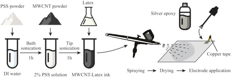
FIGURE 1. Preparation of the MWCNT-latex ink and fabrication of the pressure-sensitive foam.

First, 2 wt.% of poly (sodium 4-styrenesulfonate) (PSS) (Sigma-Aldrich) was dissolved in deionized (DI) water. Second, 0.339 g of MWCNT and 0.806 g of N-methyl-2-pyrrolidinone (NMP) (Sigma-Aldrich) were mixed with 33.855 g of 2 wt.% PSS solution. The mixture was then immersed in an ice bath and subjected to high-energy tip ultrasonication (5 s on and 5 s off; 6.35 mm tip; 30 min at 30% amplitude) for 1 h to disperse the MWCNTs. Last, the sprayable ink was finalized by adding an appropriate amount of latex solution (Kynar Aquatec) and DI water to the MWCNT dispersion.

The MWCNT-latex ink was manually spray-coated onto 214 × 230 mm² Smartfoam specimens (3 mm thick) using a Paasche airbrush. Each specimen was then air-dried at room temperature for at least 12 h before use. After the thin film was completely dry, multi-strand wires were deployed along the boundaries of the specimen using copper tape and silver epoxy (provided by MG Chemicals) to form the electrodes. A total of 26 electrodes arranged in a 6 × 7 pattern was prepared as shown in Figure 2A. Since the foam was flexible and soft, the specimen was fixed to a rigid 3D-printed PLA support.

FIGURE 2

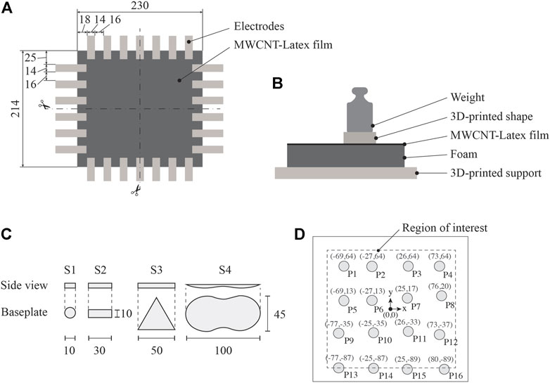
FIGURE 2. (A) Schematic of the sensing specimen and ERT boundary electrodes (B) test setup for applying pressure hotspots (C) 3D-printed shapes to control contact area; and (D) location of hotspots and coordinates of their centers. All dimensions are shown in millimeters.

Since the deposition process only involved spraying the sensing material onto the foam substrate, fabrication was easily scalable. However, it is worth noting that the resolution of conductivity images reconstructed by EIT is generally related to the properties (size and impedance) and the number of electrodes. From a practical point of view, increasing the number of electrodes leads to a longer vector of voltage measurements, which generally needs a more extensive set of trainable variables (i.e., number of RBFs in the RBFN and number of neurons and/or layers in the DNN) to reconstruct conductivity distributions at a high resolution. Moreover, large sensing areas involve longer distances in the interrogation process, increasing material resistance and, therefore, leading to smaller voltage measurements in electrodes far from those used for current injection. This may lead to a higher dependency of the results on instrumentation noise and amplify the effects of unevenly distributed conductivity (e.g., due to material defects). However, in general, these issues can be addressed by increasing the magnitude of the injected current.

5.2 Applied Pressure Test Setup

Prior to the start of any test, baseline ERT measurements of the unstrained nanocomposite-enhanced foam were obtained. ERT measurements were collected using a customized data acquisition (DAQ) system consisting of a Keithley 6221 AC/DC generator (for boundary current excitations) coupled with a Keysight 34980A multifunctional switch with an embedded digital multimeter (for switching and boundary voltage measurement). MATLAB was used to control the DAQ system using the adjacent interrogation pattern. It should be mentioned that DC was injected across a pair of boundary electrodes, while voltage magnitudes across all other adjacent pairs were recorded.

Two sets of pressure sensing tests were performed, both using the setup illustrated in Figure 2B. Test #1 was aimed at investigating whether the proposed sensing solution could accurately determine the location of pressure hotspots. In order to keep the contact area as constant as possible throughout the test, the S1 3D-printed polylactic acid (PLA) disc represented in Figure 2C with a diameter of 10 mm was inserted between a weight and the sensing specimen. A mass of 200 g was placed at 16 different positions on the nanocomposite-enhanced foam as shown in Figure 2D, and ERT measurements were obtained for each position. Test #2 aimed to characterize the accuracy of identifying different pressure shapes. In this case, three 3D-printed PLA shapes (i.e., S2, S3, and S4 shown in Figure 2C) were placed at different positions on the sensing surface. Specifically, a mass of 500 g was used for shape S2, 1 kg for shape S3, and 4 kg for shape S4. Similar to Test #1, ERT measurements were recorded after each pressure hotspot was introduced.

The foam substrate used in this study was relatively thin compared to the dimensions of the sensing area and baseplates. Besides, the latex enhanced the elastic properties of the sensing film and allowed it to adapt to foam deformation without developing significant stresses on its outer surface. Therefore, shear effects due to applied loads and in-plane stretching of the sensing surface that could arise far from the applied pressure hotspot are limited as compared to the deformation of the MWCNT-latex film in the loaded region. For this reason, the expected conductivity variations obtained through ERT were almost coincident with the shape of PLA baseplates. This result remains valid for foam substrates with a modest thickness or relatively high Poisson’s ratio.

5.3 Training Dataset for ML Methods

As explained in Section 4.1, the dataset used to train the 2 ML methods was built by numerically solving the forward problem. The nanocomposite-enhanced foam was modeled according to Figure 3A, with 9716 elements for the FE model and electrodes modeled as void areas. CEM conditions were imposed at the boundary of each electrode (i.e., at the interface between the sensing film and the silver epoxy) as shown in Figure 3A. The experimental test setup is shown in Figure 3B, and the specimen resembles the FE model.

FIGURE 3

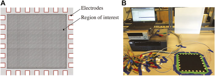
FIGURE 3. (A) FE model of the specimen and (B) experimental setup.

It is pointed out that, while unevenly distributed material may generate spatial differences in the conductivity distribution for real specimens, the training dataset was generated considering a uniform conductivity in “unloaded” regions. However, only variations in conductivity with respect to the baseline configuration are assessed by difference imaging. Therefore, if a complex conductivity pattern constitutes the baseline configuration, and an additional effect (e.g., due to load) perturbs locally the baseline conductivity distribution, only the artifact generated by the perturbing phenomenon is reconstructed by EIT. However, applying a given load to different locations may lead to different conductivity variations based on the effective distribution of the sensing material. The normalization criterion proposed in Section 4.1 aims at minimizing this effect and the differences between the simulations and real experiments.

A set of $C$ = 15,000 random polygons within a rectangular region of interest of 3,690 elements (see Figure 3A) were generated using the following parameters: $P$ = 4, $R_p$ = 70 mm, and $K_p$ = 5 with reference to Algorithm 1. The conductivity within the resulting area was reduced by a random value between 0 and 100% for each case. In order to improve the robustness of the training process, jitter was included in the training dataset with $\gamma$ = 0.01 and $S$ = 5 (see Section 4.1). The DNN used to solve the ERT inverse problem was designed as follows. After the input layer, which contains 598 neurons (i.e., the size of voltage measurements for each inspection), four hidden fully-connected layers, each containing 2048 neurons and followed by exponential linear unit activation functions, were employed. At the end of the network, a fully connected layer with 3,690 neurons without activation functions was used, which has a size equal to the number of elements that constitute the region of interest in the FE mesh.

The network was trained using the extended training set (i.e., including jitter, see Eq. 8) that contains 75,000 different cases, using the Adam optimization algorithm (Kingma and Ba, 2015). The initial learning rate was set to 0.001, since higher values led to convergence issues. Indeed, at the beginning of the training process, a large value was employed to escape spurious local minima and accelerate training. Then, a decay in the learning rate of 1/10 was considered when the root mean square reconstruction error was almost constant (i.e., after 10 epochs) to avoid oscillation around local minima. The authors also noticed that the reconstruction error was almost constant after two drops. Therefore, a total of 30 epochs was selected. The denominator offset was set to 10⁻⁸, and the decay rate of the gradient moving average was 0.9, while the batch size was 128. These parameters are recurrent in training applications (Kingma and Ba, 2015) and the results showed to be slightly affected by different values.

On the other hand, the RBF network consists of a single fully connected layer containing 100 neurons activated by Gaussian RBFs. The centers of the kernel functions were selected as the centers of 100 clusters determined using the k-means algorithm on the jittered training dataset, while the spread parameter $b$ was determined as explained in Section 4.3. The RBF network was trained by solving the least-squares problem of Eq. 15 while considering the full dataset containing 75,000 cases.

Typically, the training set is adequate for regression problems if it uniformly spans the space of the input features. Therefore, the training samples must be designed such that their shape and size represent a comprehensive set of the expected pressure hotspots (in size, shape, and location). From the perspective of scalability, if the sensing area becomes larger but the size of the expected hotspots is the same, the size of the training dataset should increase to include samples that span the input space uniformly and densely.

5.4 Results and Discussion

First, Test #1 was performed, and the datasets were used for solving the ERT inverse problem using difference imaging and the TV method. Figure 4 plots the conductivity distribution changes between each applied pressure hotspot with respect to the baseline. Specifically, an $\alpha$ factor equal to 10⁻⁶ and a single iteration of the procedure shown in Section 3 were employed to generate these results. The location of the largest conductivity variation was, in general, correctly identified, as can be seen in Figure 4 (the reference locations of applied loads are represented as dashed red circles). However, the shape and size of the pressure hotspot (i.e., using the S1 baseplate shown in Figure 2C) are not clearly visible due to the several artifacts present in the reconstructed change in conductivity distributions. It should also be noted that the magnitude of the conductivity changes (here expressed in S/m) were also inconsistent despite the applied pressure being the same. In fact, conductivity change is generally higher when the load was applied closer to the electrodes, which is consistent with previous reports of nonuniform sensitivity between the center and boundary regions (Baltopoulos et al., 2013). Overall, the average computing time to solve the ERT inverse problem using the TV method was 0.65 s using MATLAB (R2020b version) running on an Intel^® Core™ i7-8,700 6@3.20GHz-processor CPU with 2 GB NVIDIA Quadro P620 GPU, 32GB RAM, and Windows 10 operating system.

FIGURE 4

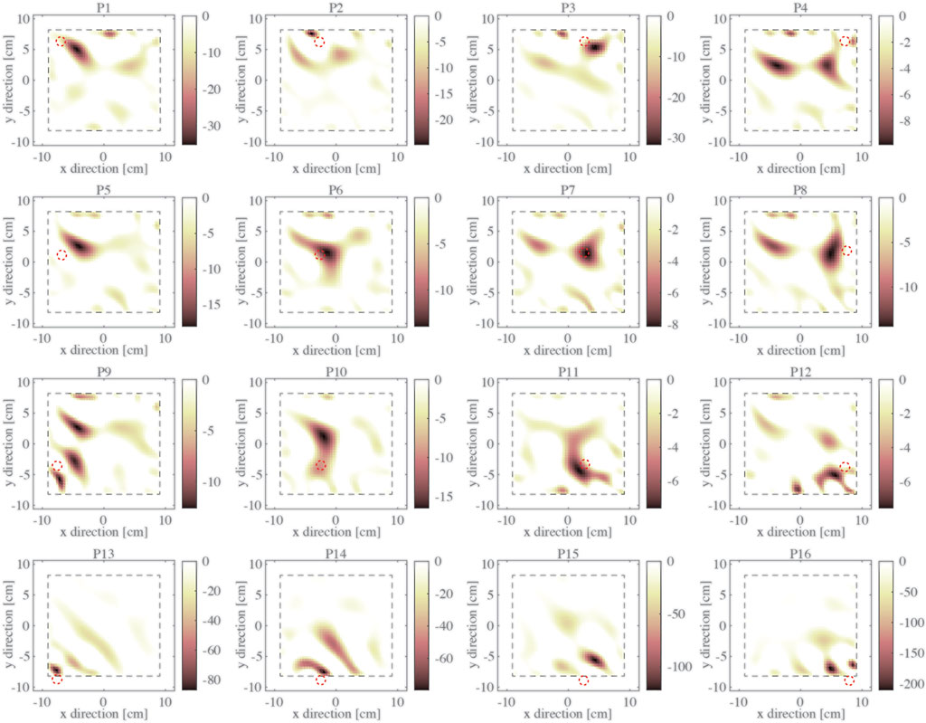
FIGURE 4. Conductivity distributions obtained using the TV method for Test #1.

On the other hand, Figures 5, 6 show the results for Test #1 when the ERT datasets were processed using the DNN and the RBFN methods, respectively. Specifically, the elements in the output vector generated by the ML algorithms are represented on a 2D map corresponding to the respective mesh elements. Compared to the results of Figure 4, the DNN-based method provides a much higher resolution of detecting pressure hotspots, where the actual size and location of the baseplate are generally accurately identified, while noise artifacts are minimized (Figure 5). The reconstruction process takes on average 0.005 s using the trained DNN running on the same hardware system (i.e., less than two orders of magnitude as compared to the TV method). This considerable improvement in computing performance is due to the nature of the feedforward process employed by DNN to solve the ERT inverse problem, which does not require performing demanding matrix inversion operations.

FIGURE 5

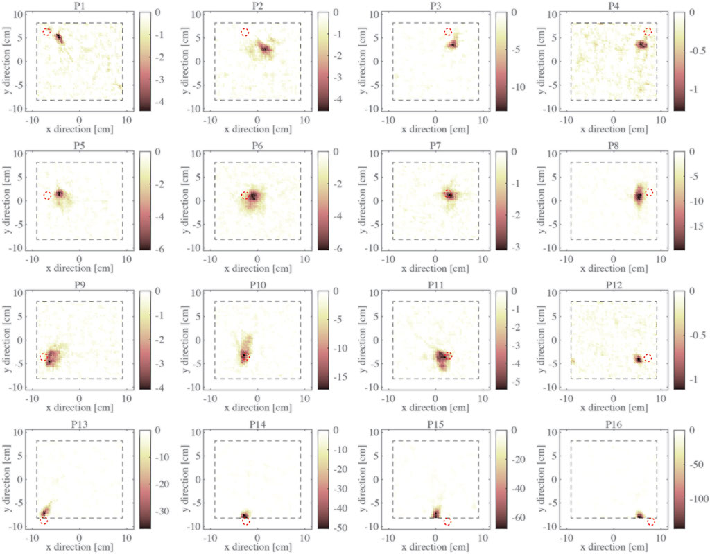
FIGURE 5. Conductivity distributions obtained using the DNN-based method for Test #1.

FIGURE 6

FIGURE 6. Conductivity distributions obtained using the RBFN-based method for Test #1.

The results obtained using RBFN in Figure 6 have a visibly lower resolution as compared to DNN (Figure 5). Although hotspot location in each image is generally well estimated, noise artifacts are more regular as compared to the results of the TV method (Figure 4). The main advantage of the RBFN-based method is its computational time, which was significantly lower and was on average 0.003 s for each reconstruction. Moreover, due to the limited number of neurons employed in the network, the RBFN has 100 weights for each output value or 369,000 weights in total. In contrast, DNN uses over 21 million weights and is difficult to track, especially when these algorithms are implemented and executed using portable computing nodes such as microcontrollers.

The DNN, with a higher number of trainable variables, has shown superior ability in accurately correlating slight and localized variations in the input (voltage measurements) to complex conductivity patterns. On the other hand, a limited set of RBFs constitutes a basis for describing the conductivity distribution in RBFNs, which can only provide a general yet robust reconstruction of the conductivity variation. The relatively large spread factor of the RBFs improves the generalization ability but makes the reconstruction of complex patterns and sharp peaks in predicted conductivity particularly challenging. Nevertheless, in general, due to the lower sensitivity to minor variations of the voltage data, RBFNs are less sensitive to noise.

Overall, both ML methods provided conductivity reduction magnitudes that are almost proportional to those obtained by the TV method, which confirmed the efficacy of the adopted normalization process. However, the estimated magnitude was not only dependent on the load but also on the location on the sensing surface. This result could be due to the uneven thickness (and hence resistance) of the sensing specimen or local phenomena that affected areas close to the electrodes.

Second, the results for Test #2 are shown in Figure 7, where Test #2 corresponded to the case when different contact pressure patterns were applied to the nanocomposite-enhanced foam. Different weights were placed onto rectangular, triangular, and figure-eight baseplates and on the sensing specimens. Figure 7 shows that, although DNN generally provides a more accurate localization and shape reconstruction for small pressure hotspots, it behaves worse for distributed loads, as is visible from the results for the figure-eight baseplate. On the other hand, good reconstruction for large distributed loads obtained through the RBFN confirms its superior generalization ability. Indeed, the maximum size of the polygons representing pressure hotspots in the training set is 70 mm, lower than the maximum size of shape S4. In this case, the result obtained using the DNN may be less accurate since the training set did not include enough samples representative of the real condition, which could only be generated by randomly combining several closely-spaced polygons.

FIGURE 7

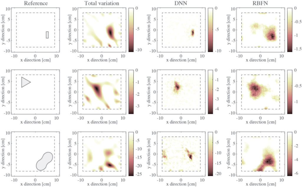
FIGURE 7. Conductivity distributions obtained for Test #2.

6 Conclusion

Pressure mapping was demonstrated using a nanocomposite-enhanced soft foam and the use of 2 ML tools, namely a DNN and an RBFN algorithm, to solve the ERT inverse problem. The DNN method provided accurate results for the identification of small hotspots while also allowing accurate shape reconstruction of the shape of the baseplate used to apply the load. Larger and more complex pressure regions are localized but without accurate shape information. On the other hand, although the RBFN did not allow accurately localize small pressure hotspots, it was more robust for identifying larger applied pressure regions. Both ML techniques performed better than the traditional total variation method, especially in terms of computational efficiency, with a runtime two orders of magnitude lower than the traditional method. The RBFN required a much smaller physical memory and computational footprint than the DNN, since network weights are about 58 times fewer and makes them more suitable for portable applications such as healthcare and robotic. The easy deployment of the sensing film, together with the modest runtime and satisfactory accuracy of the ML-based mapping algorithms, make the proposed solution promising for portable applications (e.g., running on low-cost microcontrollers), especially when the exact shape of the pressure hotspot is not of fundamental interest, such as in most medical applications.

Data Availability Statement

The raw data supporting the conclusion of this article will be made available by the authors, without undue reservation.

Author Contributions

All authors conceived the idea. SL and KL contributed to specimen design and fabrication. SL and SQ conducted the experiments. SQ and YS implemented the algorithms. SQ and YS analyzed the results, while SQ wrote the draft paper while collecting input from all other authors. KL supervised the research and edited the manuscript.

Funding

This research was partially supported by the United States Office of Naval Research (ONR) under grant number N00014-20-1-2329 (principal investigator: KL), as well as the University of California San Diego, Jacobs School of Engineering. SQ (working under Ph.D. advisor Prof. Luca Landi), and his visiting scholar appointment at UC San Diego and the ARMOR Lab, was supported by the University of Bologna, through the Marco Polo program.

Conflict of Interest

The authors declare that the research was conducted in the absence of any commercial or financial relationships that could be construed as a potential conflict of interest.

Publisher’s Note

All claims expressed in this article are solely those of the authors and do not necessarily represent those of their affiliated organizations, or those of the publisher, the editors and the reviewers. Any product that may be evaluated in this article, or claim that may be made by its manufacturer, is not guaranteed or endorsed by the publisher.

References

An, G. (1996). The Effects of Adding Noise during Backpropagation Training on a Generalization Performance. Neural Comput. 8, 643–674. doi:10.1162/neco.1996.8.3.643

CrossRef Full Text | Google Scholar

Baltopoulos, A., Polydorides, N., Pambaguian, L., Vavouliotis, A., and Kostopoulos, V. (2013). Damage Identification in Carbon Fiber Reinforced Polymer Plates Using Electrical Resistance Tomography Mapping. J. Compos. Mater. 47, 3285–3301. doi:10.1177/0021998312464079

CrossRef Full Text | Google Scholar

Bishop, C. M. (1995). Training with Noise Is Equivalent to Tikhonov Regularization. Neural Comput. 7, 108–116. doi:10.1162/neco.1995.7.1.108

CrossRef Full Text | Google Scholar

Calderón, A. P. (2006). On an Inverse Boundary Value Problem. Comput. Appl. Math. 25, 133–138. doi:10.1590/S0101-82052006000200002

CrossRef Full Text | Google Scholar

Dai, H., and Thostenson, E. T. (2019). Large-Area Carbon Nanotube-Based Flexible Composites for Ultra-Wide Range Pressure Sensing and Spatial Pressure Mapping. ACS Appl. Mater. Inter. 11, 48370–48380. doi:10.1021/acsami.9b17100

PubMed Abstract | CrossRef Full Text | Google Scholar

D. Holder (Editor) (2004). Electrical Impedance Tomography - Methods, History and Applications (Boca Raton, FL, United States: CRC Press).

Google Scholar

Ding, Y., Yang, J., Tolle, C. R., and Zhu, Z. (2018). Flexible and Compressible PEDOT:PSS@Melamine Conductive Sponge Prepared via One-Step Dip Coating as Piezoresistive Pressure Sensor for Human Motion Detection. ACS Appl. Mater. Inter. 10, 16077–16086. doi:10.1021/acsami.8b00457

PubMed Abstract | CrossRef Full Text | Google Scholar

Duan, X., Taurand, S., and Soleimani, M. (2019). Artificial Skin through Super-Sensing Method and Electrical Impedance Data from Conductive Fabric with Aid of Deep Learning. Sci. Rep. 9, 8831. doi:10.1038/s41598-019-45484-6

PubMed Abstract | CrossRef Full Text | Google Scholar

Frerichs, I., Amato, M. B. P., van Kaam, A. H., Tingay, D. G., Zhao, Z., Grychtol, B., et al. (2017). Chest Electrical Impedance Tomography Examination, Data Analysis, Terminology, Clinical Use and Recommendations: Consensus Statement of the TRanslational EIT developmeNt stuDy Group. Thorax 72, 83–93. doi:10.1136/thoraxjnl-2016-208357

PubMed Abstract | CrossRef Full Text | Google Scholar

Gupta, S., Gonzalez, J. G., and Loh, K. J. (2017). Self-Sensing Concrete Enabled by Nano-Engineered Cement-Aggregate Interfaces. Struct. Health Monit. 16, 309–323. doi:10.1177/1475921716643867

CrossRef Full Text | Google Scholar

Huang, Z., Gao, M., Yan, Z., Pan, T., Khan, S. A., Zhang, Y., et al. (2017). Pyramid Microstructure with Single Walled Carbon Nanotubes for Flexible and Transparent Micro-Pressure Sensor with Ultra-high Sensitivity. Sensors Actuators A: Phys. 266, 345–351. doi:10.1016/j.sna.2017.09.054

CrossRef Full Text | Google Scholar

Husain, Z., Madjid, N. A., and Liatsis, P. (2021). Tactile Sensing Using Machine Learning-Driven Electrical Impedance Tomography. IEEE Sensors J. 21, 11628–11642. doi:10.1109/JSEN.2021.3054870

CrossRef Full Text | Google Scholar

Kim, K., Jung, M., Jeon, S., and Bae, J. (2019). Robust and Scalable Three-Dimensional Spacer Textile Pressure Sensor for Human Motion Detection. Smart Mater. Struct. 28, 065019. doi:10.1088/1361-665X/ab1adf

CrossRef Full Text | Google Scholar

Kingma, D. P., and Ba, J. L. (2015). “Adam: A Method for Stochastic Optimization,” in 3rd International Conference on Learning Representations, ICLR 2015 - Conference Track Proceedings, San Diego, CA, USA, 7–9 May 2015.

Google Scholar

Lee, H., Park, K., Kim, J., and Kuchenbecker, K. J. (2021). Piezoresistive Textile Layer and Distributed Electrode Structure for Soft Whole-Body Tactile Skin. Smart Mater. Struct. 30, 085036. doi:10.1088/1361-665X/ac0c2e

CrossRef Full Text | Google Scholar

Li, S., Lin, Y.-A., and Loh, K. J. (2021). “Pressure Mapping Using a Smart Nanocomposite Foam and Electrical Impedance Tomography,” in Nano-, Bio-, Info-Tech Sensors and Wearable Systems, California, United States, 22–27 March 2021. Editor J. Kim (SPIE), 5. doi:10.1117/12.2582872

CrossRef Full Text | Google Scholar

Lin, Y. A., Zhao, Y., Wang, L., Park, Y., Yeh, Y. J., Chiang, W. H., et al. (2021). Graphene K‐Tape Meshes for Densely Distributed Human Motion Monitoring. Adv. Mater. Technol. 6, 2000861. doi:10.1002/admt.202000861

CrossRef Full Text | Google Scholar

Lin, Z., Guo, R., Zhang, K., Li, M., Yang, F., Xu And, S., et al. (2020). Neural Network-Based Supervised Descent Method for 2D Electrical Impedance Tomography. Physiol. Meas. 41, 074003. doi:10.1088/1361-6579/ab9871

PubMed Abstract | CrossRef Full Text | Google Scholar

Liu, Z., Zhang, T., Yang, M., Gao, W., Wu, S., Wang, K., et al. (2021). Hydrogel Pressure Distribution Sensors Based on an Imaging Strategy and Machine Learning. ACS Appl. Electron. Mater. 3, 3599–3609. doi:10.1021/acsaelm.1c00488

CrossRef Full Text | Google Scholar

Loh, K. J., Hou, T.-C., Lynch, J. P., and Kotov, N. A. (2009). Carbon Nanotube Sensing Skins for Spatial Strain and Impact Damage Identification. J. Nondestruct Eval. 28, 9–25. doi:10.1007/s10921-009-0043-y

CrossRef Full Text | Google Scholar

Loyola, B. R., Saponara, V. L., Loh, K. J., Briggs, T. M., O'Bryan, G., and Skinner, J. L. (2013). Spatial Sensing Using Electrical Impedance Tomography. IEEE Sensors J. 13, 2357–2367. doi:10.1109/JSEN.2013.2253456

CrossRef Full Text | Google Scholar

Nela, L., Tang, J., Cao, Q., Tulevski, G., and Han, S.-J. (2018). Large-Area High-Performance Flexible Pressure Sensor with Carbon Nanotube Active Matrix for Electronic Skin. Nano Lett. 18, 2054–2059. doi:10.1021/acs.nanolett.8b00063

PubMed Abstract | CrossRef Full Text | Google Scholar

Reed, R. D., and Marks, R. J. (1998). Neural Smithing: Supervised Learning in Feedforward Artificial Neural Networks. Cambridge, MA, USA: MIT Press.

Google Scholar

Ryu, H., Park, S., Park, J.-J., and Bae, J. (2018). A Knitted Glove Sensing System with Compression Strain for Finger Movements. Smart Mater. Struct. 27, 055016. doi:10.1088/1361-665X/aab7cc

CrossRef Full Text | Google Scholar

Shirinov, A. V., and Schomburg, W. K. (2008). Pressure Sensor from a PVDF Film. Sensors Actuators A: Phys. 142, 48–55. doi:10.1016/j.sna.2007.04.002

CrossRef Full Text | Google Scholar

Tallman, T. N., and Smyl, D. J. (2020). Structural Health and Condition Monitoring via Electrical Impedance Tomography in Self-Sensing Materials: A Review. Smart Mater. Struct. 29, 123001. doi:10.1088/1361-665X/abb352

CrossRef Full Text | Google Scholar

Tao, L.-Q., Zhang, K.-N., Tian, H., Liu, Y., Wang, D.-Y., Chen, Y.-Q., et al. (2017). Graphene-Paper Pressure Sensor for Detecting Human Motions. ACS Nano 11, 8790–8795. doi:10.1021/acsnano.7b02826

PubMed Abstract | CrossRef Full Text | Google Scholar

Wang, H., Liu, K., Wu, Y., Wang, S., Zhang, Z., Li, F., et al. (2021). Image Reconstruction for Electrical Impedance Tomography Using Radial Basis Function Neural Network Based on Hybrid Particle Swarm Optimization Algorithm. IEEE Sensors J. 21, 1926–1934. doi:10.1109/JSEN.2020.3019309

CrossRef Full Text | Google Scholar

Wang, L., Gupta, S., Loh, K. J., and Koo, H. S. (2016). Distributed Pressure Sensing Using Carbon Nanotube Fabrics. IEEE Sensors J. 16, 4663–4664. doi:10.1109/JSEN.2016.2553045

CrossRef Full Text | Google Scholar

Wang, L., and Loh, K. J. (2016). Spray-Coated Carbon Nanotube-Latex Strain Sensors. Sci. Lett. J. 5, 234.

Google Scholar

Wu, X., Han, Y., Zhang, X., Zhou, Z., and Lu, C. (2016). Large-Area Compliant, Low-Cost, and Versatile Pressure-Sensing Platform Based on Microcrack-Designed Carbon Black@Polyurethane Sponge for Human-Machine Interfacing. Adv. Funct. Mater. 26, 6246–6256. doi:10.1002/adfm.201601995

CrossRef Full Text | Google Scholar

Yao, A., and Soleimani, M. (2012). A Pressure Mapping Imaging Device Based on Electrical Impedance Tomography of Conductive Fabrics. Sens Rev. 32, 310–317. doi:10.1108/02602281211257542

CrossRef Full Text | Google Scholar

Zang, Y., Zhang, F., Di, C.-A., and Zhu, D. (2015). Advances of Flexible Pressure Sensors toward Artificial Intelligence and Health Care Applications. Mater. Horiz. 2, 140–156. doi:10.1039/C4MH00147H

CrossRef Full Text | Google Scholar