A Structural Damage Identification Method Based on Arrangement of the Static Force Residual Vector

1 Introduction

As a modern green building, steel structure is widely used in building and transportation infrastructure because of its light weight, high strength, strong seismic performance, short construction period, and less environmental pollution (Han and Shi, 2012; Shi et al., 2020; Han et al., 2021). However, with the extension of the service life of the structure, the damage of the structure often brings potential safety hazards. They are vulnerable to damage due to dangerous conditions such as aging, load changes, environmental corrosion, and earthquakes (OBrien and Malekjafarian, 2016; Wang et al., 2018; Eftekhar Azam et al., 2019). One or more components of the structure may be damaged, so the system cannot work normally. As these defects expand in structural members, the safety decreases, resulting in the possible failure of members or the whole structure.

In order to avoid this situation, it becomes more important to monitor the health of infrastructures such as steel buildings and steel bridges. The traditional condition evaluation of steel structure buildings and steel bridges is mainly carried out through visual inspection. In order to detect structural damage as early as possible and prevent structural failure, it is necessary to carry out continuous intelligent health monitoring of the structure. Reliable and effective nondestructive identification can ensure the safety and integrity of the structure (Link and Zimmerman, 2015; Eun-Taik and Hee-Chang, 2018; Truong et al., 2020; Mousavi et al., 2021). However, there are many problems in using timely recorded data to estimate the location and severity of structural damage. In the existing damage detection methods, the most common method is the method based on vibration. In the past few decades, these methods have attracted more and more attention. The principle behind these methods is based on the fact that damage will change structural characteristics, such as stiffness, mass, flexibility, and damping. The changes in these structural characteristics change the dynamic parameters of the structure, such as natural frequency and vibration mode (Nguyen et al., 2016; Pérez and Serra-López, 2019). These changes in structure and modal parameters can be used as indicators of structural damage detection. These techniques are based on the features extracted from modal parameters. They are divided into the following categories: methods based on natural frequency, methods based on modal shape, methods based on curvature/strain modal shape, and other methods based on modal parameters (Rucevskis et al., 2016). In the past few years, a large number of studies on damage identification of various structures based on vibration methods have been completed, such as beams (Huang et al., 2019; He et al., 2021), plate structures (Gomes et al., 2019; Huang and Schröder, 2021), trusses (Azim and Gül, 2021; Zhuo and Cao, 2021), and bridges (Azim and Gül, 2021; Zhan et al., 2021).

In general, structural damage detection is mainly used to identify the location and damage level of the structure. In the process of identification, the response of the external excitation is measured by a dynamic test or static test. Therefore, the damage is usually directly identified by numerical operation. The result of structural damage is the reduction of the local stiffness of the structure. Therefore, the damage of the structure can be regarded as a change in stiffness, ignoring the change in quality, and can be detected by changes in dynamic or static characteristics (Di Paola and Bilello, 2004; Huynh et al., 2005; Wei Fan and Pizhong Qiao, 2011; Abdo, 2012; Sung et al., 2013).

Considering the nature of the measurement data, the measurement methods can be divided into two categories: dynamic methods and static methods. Due to the convenience of dynamic data measurement, several damage identification methods have been developed on the basis of dynamic testing (Cornwell et al., 1999; Abdo and Hori, 2002; Debruyne et al., 2015; Nogal et al., 2016). Many experts have conducted extensive research on damage identification using the residual force vector method under dynamic response. Zimmerman and Kaouk (1992) first proposed the theoretical algorithm related to the residual force vector method. Kahl and Sirkis (1996) improved the theoretical algorithm proposed by the former and identified the damage location in the beam member. Li et al. (2016) used the difference of the virtual residual force vector of the intact structure and the damaged structure to locate the damage location, combined with the response sensitivity method to identify the local damage degree, and better identified the location and damage degree of single damage and multiple damages. Nobahari et al. (2018) used the concept of residual force vector and proposed a method based on the damage index of truss units. This method can find the most likely damaged component location, and eliminate the undamaged units from all variables to reduce the amount of calculation, and then use the genetic algorithm to find a more specific damaged unit in the concentrated position of the damaged component and calculate its damage degrees.

The purpose of dynamic analysis is to determine the parameters such as internal force, stress, and displacement under dynamic load. In vibration modal analysis, the main calculation work is to solve the Eigen problem, which requires more calculation work than static analysis (Kirsch, 2003). The general residual force vector method for damage identification is mainly based on the modal parameters of the dynamic test, which requires a more complicated modal analysis, and the accuracy of the damage analysis results is not high. Based on the residual force vector method under dynamic response, this article proposes a force residual vector method. This method uses the sparse property of the damage unit stiffness matrix and its corresponding residual vector distribution rule to realize the location of the damaged unit and gives the damage degree after the location by solving the self-balance equation of the damaged unit. In this study, numerical examples of simply supported beams and trusses have been verified, and the damage location and damage degree of the structure have been identified. In order to verify the necessity of structural damage identification, the dynamic responses of the original model and the damaged truss model are simulated and compared by using the state space theory under the action of the El Centro seismic wave.

2 Theory of Force Residual Vector Method

2.1 Basic Assumptions

In damage identification with the force residual vector method, it is necessary to make some basic assumptions about the structure:

(1) When the structure is damaged, only the rigidity of the structure is reduced, and the influence of quality on the structure is ignored.

(2) The damage of structural units is discontinuous in the finite element model. This assumption has been given in previous studies (Kasper et al., 2008; Zhang et al., 2009).

2.2 Theoretical Equations

A structural system produces node displacement D under the action of static force F. The static equilibrium equation in the global coordinate system can be expressed as the following formula:

$\mathit{KD}=\mathit{F}(1)$

where K is the global stiffness matrix of the structural system, and D is the node displacement vector in the global coordinate system.

When the structure is damaged, its stiffness matrix will change. Assuming that ${\alpha }_i$ is the damage degree of the stiffness matrix corresponding to the $\mathit{i}-th$ structural unit, the perturbation matrix △K of structural damage can be expressed as the following formula:

$\mathrm{\Delta }\mathit{K}=\alpha \mathit{K}(2)$

where α is the damage degree vector.

Substituting the damage stiffness △K and the displacement d of the structure after damage into Equation 1, we get the following formula:

$\left(\mathit{K}-\mathrm{\Delta }\mathit{K}\right)d=\mathit{F}(3)$

For Equation 3, moving the term without △K to the right side of the equation, we get the following equation.

$\mathrm{\Delta }\mathit{K}d=\mathit{K}d-\mathit{F}(4)$

The vector on the right side of Eq. 4 is defined as the force residual vector P:

$\mathit{K}d-\mathit{F}=\mathit{P}={\left[\begin{array}{cccc}{p}_1& p_2& \cdots & p_{\mathrm{n}}\end{array}\right]}^{{\rm T}}(5)$

The values of elements p_i corresponding to the damaged units in the P vector are much larger than those of the undamaged units. The values of elements p_i corresponding to the undamaged unit approach 0. That can be used as a filtering condition in the analysis process. The elements in the vector P of Eq. 5 are arranged in descending order of their absolute values. The structure units with larger values in front are corresponding to the damaged units. It can be used to realize localization of damage unit precisely.

Equation 5 is composed of n equilibrium equations at nodes, suppose that there is a unit damage on a node and that the elements p_i values, the unit stiffness matrix, and the displacement vector are proportional for a given damage unit, then the ratio is the damage degree. It can be realized identification of damage degree. Therefore, the damage coefficient can be obtained according to the following formula:

${\alpha }_i{\mathit{K}}_{i}d=P_i(6)$

where K_i is the global stiffness matrix containing only the unit stiffness matrix elements of the damage unit.

2.3 State Space Theory

State space representation is a mathematical model that represents a physical system as a set of inputs, outputs, and states, and the relationship between inputs, outputs, and states can be described by many first-order differential equations. For a damped system with n degrees of freedom, the dynamic differential equation can be expressed as follows:

$\mathit{M}\ddot{u}\left(t\right)+{\mathit{C}}_0\dot{u}\left(t\right)+\mathit{K}u\left(t\right)=\mathit{U}\left(t\right)(7)$

where M is the mass matrix of the structure, C₀ is the damping matrix of the structure, K is the stiffness matrix of the structure, U(t) is the load vector at t, and $\ddot{u}\left(t\right)$、, $\dot{u}\left(t\right)$, and $u\left(t\right)$ are the acceleration, velocity, and displacement responses at t, respectively.

Both sides of Equation 7 are multiplied by M⁻¹ at the same time, which can be expressed as follows:

$\ddot{u}\left(t\right)+{\mathit{M}}^{-1}{\mathit{C}}_0\dot{u}\left(t\right)+{\mathit{M}}^{-1}\mathit{K}u\left(t\right)={\mathit{M}}^{-1}\mathit{U}\left(t\right)(8)$

Finishing Equation 8 can Be Expressed as follows:

$\ddot{u}\left(t\right)=-{\mathit{M}}^{-1}\mathit{K}u\left(t\right)-{\mathit{M}}^{-1}{\mathit{C}}_0\dot{u}\left(t\right)+{\mathit{M}}^{-1}\mathit{U}\left(t\right)(9)$

Define the state vector, which can be expressed as follows:

$\mathit{X}\left(t\right)={\left[\begin{array}{cc}u\left(t\right)& \dot{u}\left(t\right)\end{array}\right]}^{{\rm T}}(10)$

The derivation of the state vector can be expressed as follows:

$\dot{\mathit{X}}\left(t\right)={\left[\begin{array}{cc}\dot{u}\left(t\right)& \ddot{u}\left(t\right)\end{array}\right]}^{{\rm T}}(11)$

Combined Equations 9–11 can be expressed as:

$\begin{array}{l}\dot{\mathit{X}}\left(t\right)=\left[\begin{array}{c}\dot{u}\left(t\right)\\ -{\mathit{M}}^{-1}\mathit{K}u\left(t\right)-{\mathit{M}}^{-1}{\mathit{C}}_0\dot{u}\left(t\right)+{\mathit{M}}^{-1}U\left(t\right)\end{array}\right]\\ =\left[\begin{array}{cc}0& \mathit{N}\\ -{\mathit{M}}^{-1}\mathit{K}& -{\mathit{M}}^{-1}{\mathit{C}}_0\end{array}\right]\mathit{X}\left(t\right)+\left[\begin{array}{c}0\\ {\mathit{M}}^{-1}\end{array}\right]\mathit{U}\left(t\right)\end{array}(12)$

where N is the unit matrix.

${\mathit{A}}_{\text{c}}$ and ${\mathit{B}}_{\text{c}}$ are obtained from Equation 12, which can be expressed as follows:

${\mathit{A}}_{\mathrm{c}}=\left[\begin{array}{cc}0& \mathit{N}\\ -{\mathit{M}}^{-1}\mathit{K}& -{\mathit{M}}^{-1}{\mathit{C}}_0\end{array}\right],{\mathit{B}}_{\mathrm{c}}=\left[\begin{array}{c}0\\ {\mathit{M}}^{-1}\end{array}\right](13)$

Combined Equations 12 and 13 can be expressed as follows:

$\dot{\mathit{X}}\left(t\right)={\mathit{A}}_{\mathrm{c}}\mathit{X}\left(t\right)+{\mathit{B}}_{\mathrm{c}}\mathit{U}\left(t\right)(14)$

where A_c is the state matrix of structural continuous time system, and ${\mathit{B}}_{\text{c}}$ is the input matrix of structural continuous time system.

${\mathit{C}}_{\text{a}}$, ${\mathit{C}}_{\text{v}}$, and ${\mathit{C}}_{\text{d}}$ are acceleration output matrix, velocity output matrix, and displacement output matrix, respectively, then the output response Y (t) can be expressed as follows:

$\mathit{Y}\left(t\right)={\mathit{C}}_{\mathrm{a}}\ddot{u}\left(t\right)+{\mathit{C}}_{\mathrm{v}}\dot{u}\left(t\right)+{\mathit{C}}_{\mathrm{d}}u\left(t\right)(15)$

Combined Equations 8–15 can be expressed as follows:

$\mathit{Y}\left(t\right)=\left[\begin{array}{cc}{\mathit{C}}_{\mathrm{d}}-{\mathit{C}}_{\mathrm{a}}{\mathit{M}}^{-1}\mathit{K}& {\mathit{C}}_{\mathrm{v}}-{\mathit{C}}_{\mathrm{a}}{\mathit{M}}^{-1}{\mathit{C}}_0\end{array}\right]\left[\begin{array}{c}u\left(t\right)\\ \dot{u}\left(t\right)\end{array}\right]+{\mathit{C}}_{\mathrm{a}}{\mathit{M}}^{-1}\mathit{U}\left(t\right)(16)$

According to Equation 16, C_c and D_c can be expressed as follows:

${\mathit{C}}_{\mathrm{c}}=\left[\begin{array}{cc}{\mathit{C}}_{\mathrm{d}}-{\mathit{C}}_{\mathrm{a}}{\mathit{M}}^{-1}\mathit{K}& {\mathit{C}}_{\mathrm{v}}-{\mathit{C}}_{\mathrm{a}}{\mathit{M}}^{-1}\mathit{C}\end{array}\right],{\mathit{D}}_{\mathrm{c}}={\mathit{C}}_{\mathrm{a}}{\mathit{M}}^{-1}(17)$

According to Equation 17, it can be expressed as follows:

$\mathit{Y}\left(t\right)={\mathit{C}}_{\mathrm{c}}\mathit{X}\left(t\right)+{\mathit{D}}_{\mathrm{c}}\mathit{U}\left(t\right)(18)$

where C_c is the structure state observation matrix, and D_c is the structure input observation matrix.

The continuous time state space model (Emmert et al., 2016; Rangapuram et al., 2018; Silva et al., 2020; Varanasi and Jampana, 2020) of the system can be expressed as follows:

$\dot{\mathit{X}}\left(t\right)={\mathit{A}}_{\mathrm{c}}\mathit{X}\left(t\right)+{\mathit{B}}_{\mathrm{c}}\mathit{U}\left(t\right)(19)$

$\mathit{Y}\left(t\right)={\mathit{C}}_{\mathrm{c}}\mathit{X}\left(t\right)+{\mathit{D}}_{\mathrm{c}}\mathit{U}\left(t\right)(20)$

Because the output response of the measured structure is collected according to the sampling frequency, there is a specific sampling time interval, that is, the output response is discrete in time. Therefore, the state space model of the discrete-time system should be adopted. Under k sampling points, the discrete-time state space model of the system can be expressed as follows:

$\mathit{X}\left[k+1\right]=\mathit{AX}\left[k\right]+\mathit{BU}\left[k\right](21)$

$\mathit{Y}\left[k\right]=\mathit{CX}\left[k\right]+\mathit{DU}\left[k\right](22)$

The state matrix of the discrete-time system is $A=e^{Ac\Delta t}$, the input matrix of the discrete-time system is $B=A_{\text{c}}^{-1}\left(A-N\right)B_{\text{c}}$, the observation matrix of the discrete-time system is $C=[\begin{array}{cc}{C}_{\text{d}}{-\text{C}}_{\text{a}}{\text{M}}^{-1}\text{K}& C_v-C_a{M}^{-1}{\mathit{C}}_0\end{array}]$, and the input observation matrix is $D=D_{\text{c}}{=\text{C}}_{\text{a}}{\text{M}}^{-1}$.

2.4 Solving Steps

The specific solving steps of this method are as follows:

(1) Establish a stiffness matrix for the target structure and combine the static balance equation to obtain the force residual vector P.

(2) List the elements of vector P according to their corresponding degrees of freedom of structure units, and arrange them in descending order of absolute value.

(3) For the arranged absolute value sequence, divide the previous element by the next element. The position where the quotient obtained by the calculation tends to infinity is the last damaged unit, and the value of the degree of freedom about the last damaged unit is expressed as the total amount of degree of freedom about the damaged units. According to the fact that a structure unit has four degrees of freedom, the number of damaged units can be judged.

(4) For the elements in the list arranged according to the structure unit number, the structure unit whose ratio of the vector value corresponding to the first displacement and the third displacement equals -1 is the damaged unit so that the damaged unit is located. In addition, verify the judgment result of step (3).

(5) Take out the structure unit stiffness matrix of the located damage unit in the global coordinate system, establish the node balance equation one by one according to the number of the damaged units, and solve the damage degree of each unit according to Equation 6 to determine the damage level of the structural member.

(6) The dynamic responses of the original model and the damage model are analyzed by using the state space theory, and the corresponding peak values of displacement, velocity, and acceleration are obtained. The dynamic responses of the original model and the damage model are analyzed by using the state space theory, and the corresponding peak values of displacement, velocity, and acceleration are obtained. Then calculate the relative difference of the corresponding peaks, and summarize the analysis.

Figure 1 shows the flow chart of the specific solving steps of this method.

FIGURE 1

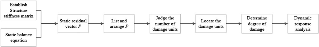
FIGURE 1. Flow chart of calculation.

3 Numerical Model Examples

In order to apply the force residual vector to practice, the following takes simply supported beams and truss structures as examples for numerical model calculations. The structural form of the two engineering examples adopts steel structure. First, we set the degrees of damage of some structural units and calculate the displacements of the structural unit nodes by calculating the force residual vector. Then the node displacements are used to locate the damaged units and determine the degrees of damage. If the identified location and the identified degrees of damage are consistent with the set values, it can show that the force residual vector method can be used to identify the damage location and the damage degree of the structure through the values of node displacements.

3.1 Numerical Model Example of Simply Supported Beam

3.1.1 Calculated Displacement Value of Simply Supported Beam

Take the simply supported beam model shown in Figure 2 as an example to explain the proposed method. The simply supported beam structure is divided into 12 units, and then the finite element analysis for it is carried out. The basic parameters of No.14 I-beam are as follows: unit length L = 0.1 m, cross-sectional area A = 2.15 × 10⁻³ m², elastic modulus E = 200 GPa, moment of inertia I = 7.12 × 10⁻⁶ m⁴, and density ρ = 7.8 × 10³ kg/m³. The simply supported beam model structure added a downward force F = 10 kN in the middle of the span, constrained the horizontal and vertical displacement at node 1, and constrained the vertical displacement at node 13.

FIGURE 2

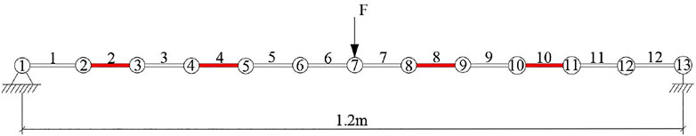
FIGURE 2. Sketch of simply supported beam.

Regardless of the axial displacement of the simply supported beam model, the stiffness matrix of the beam units related to the vertical and angular displacement is taken as follows:

${\mathit{K}}_{\mathrm{e}}=\frac{EI}{L^3}\left[\begin{array}{cccc}12& 6L& -12& 6L\\ 6L& 4L^2& -6L& 2L^2\\ -12& -6L& 12& -6L\\ 6L& 2L^2& -6L& 4L^2\end{array}\right](23)$

According to the degrees of damage ${\alpha }_i$ (0 < ${\alpha }_i$ < 1) introduced Eq. 2, the global stiffness matrix of the beam can be expressed as follows:

$\mathit{K}={\displaystyle \sum _{i=1}^{12}\left(1-{\alpha }_i\right)}{\mathit{K}}_i(24)$

where K_i represents the $i-th$ unit stiffness matrix in the global coordinate system, and the subscript $i$ represents the unit number.

Table 1 shows the node numbers and the numbers of the node degrees of freedom of simply supported beam units.

TABLE 1

TABLE 1. Node number and number of node degrees of freedom of units.

Take multiple damage case as an example: the loss of stiffness is 15% for unit 2, 60% for unit 4, 13% for unit 8, and 30% for unit 10, that is, α₂ = 0.15、α₄ = 0.60、α₈ = 0.13, and α₁₀ = 0.30.

The node displacements are calculated according to Equation 3 and arranged in Table 2 according to the order of degrees of freedom of the units. In the table, $v_{\text{a}}$ and ${\theta }_{\text{a}}$ are the vertical and rotational displacements of the left node of unit, while $v_{\text{b}}$ and ${\theta }_{\text{b}}$ are the vertical and rotational displacements of the right node of unit.

TABLE 2

TABLE 2. Node displacement of simply supported beam (mm).

Figure 3 shows the deformation diagram of the simply supported beam. In the figure, the dotted lines present the original structure, and the solid lines present the deformed structure.

FIGURE 3

FIGURE 3. Deformation diagram of simply supported beam.

3.1.2 Damage Identification of Simply Supported Beam

The calculated node displacements in Table 2 are used as the known values of structural damage identification.

The force residual vector P is determined according to Equation 5 and shown in Table 3.

TABLE 3

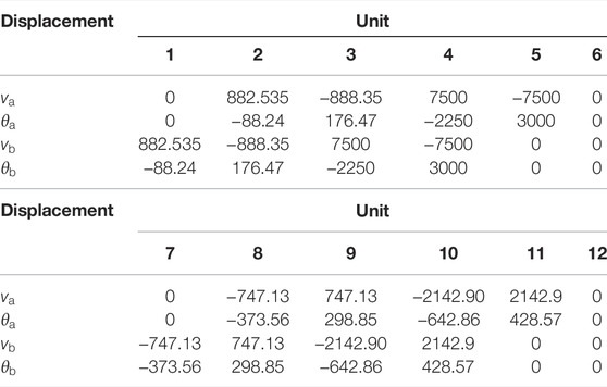
TABLE 3. Values of force residual vector P (N).

Figure 4 shows the distribution and arrangement of force residual vector P.

FIGURE 4

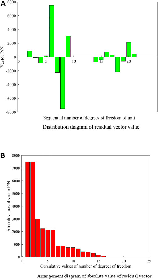
FIGURE 4. Distribution and arrangement of residual vector values of simply supported beam. (A) Distribution diagram of residual vector value (B) Arrangement diagram of the absolute value of the residual vector

Figure 4A presents the distribution of force residual vector P. The abscissa represents, from left to right, the sequential number of vertical and rotational degrees of freedom of unit nodes. The ordinate corresponds to the force residual vector of corresponding units. Figure 4B shows the arrangement of the absolute values of P in descending order. The abscissa represents the cumulative values of the number of vertical and rotational degrees of freedom of unit left and right nodes (the total number of degrees of freedom of unit nodes, including vertical degrees of freedom and corner degrees of freedom).

For the arranged absolute value sequence in Figure 4B, by dividing the previous element by the next element, we obtain the positioning diagram shown in Figure 5. The vertical coordinate of Figure 5 is expressed as the ratio of the absolute value P of the residual force vector corresponding to the first displacement and the third displacement in the element. The maximum ratio, which represents the total number of degrees of freedom of the damage units, is located at 16. Since each unit corresponds to 4 degrees of freedom in the local coordinate system, it can be seen that four units in the simply supported beam have been damaged, which is consistent with the set number of damaged units.

FIGURE 5

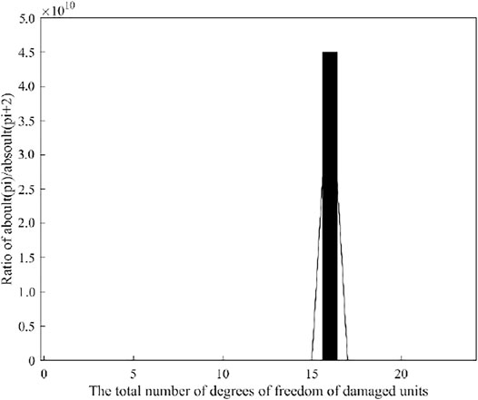
FIGURE 5. Total number of freedom degrees of damage elements.

In Table 3, the units 2, 4, 8, and 10, whose ratio of the residual vector values P corresponding to the first displacement and the third displacement of the units is -1, are damaged units. Those located damage units are the same as the set damage units.

The identification values of damage degrees are obtained by solving damage degrees using Equation 6, and the setting values of the corresponding units are listed in Table 4.

TABLE 4

TABLE 4. Identification values and setting values of unit damage degrees of simply supported beam.

It can be seen from Table 4 that all the identification values of damage degrees are completely consistent with the corresponding setting values. It can be concluded that the force residual vector method can be used to locate the damage position and identify the damage degree of the simply supported beam structure.

3.1.3 Dynamic Response Analysis of Simply Supported Beam

Dynamic response is the dynamic characteristic of the reactive structure under external excitation. The dynamic responses of the original model of the simply supported beam and the damage model of the simply supported beam under the action of the El Centro seismic wave are simulated and analyzed by using the state space theory, and the dynamic response degree of the structure under the action of the original model and the damage model is verified. Parameter setting of dynamic response analysis in this example: sampling frequency F_s = 50 Hz, sampling interval △t = 1/F_s = 0.01 s, number of generated samples N = 2500, El Centro seismic wave is a wave in the east–west direction. Figure 6 shows the time history curve of El Centro seismic excitation applied to the model. Figure 7 shows the displacement, velocity, and acceleration output dynamic response of the original model of a simply supported beam. Figure 8 shows the dynamic response of displacement, velocity, and acceleration output of the damage model of a simply supported beam, and the peak values of the dynamic response in Figures 7 and 8 are the maximum values of dynamic response of displacement, velocity, and acceleration output.

FIGURE 6

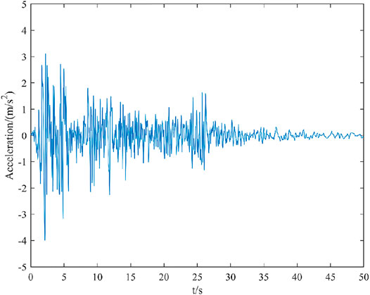
FIGURE 6. EL Centro seismic wave time history curve.

FIGURE 7

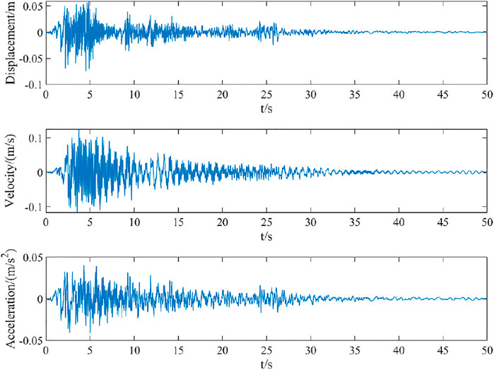
FIGURE 7. Dynamic response of displacement, velocity, and acceleration output of the original model of simply supported beam.

FIGURE 8

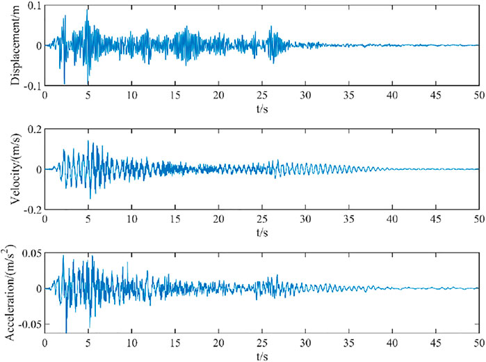
FIGURE 8. Dynamic response of displacement, velocity, and acceleration output of damage model of simply supported beam.

It can be seen from Figure 7 that under the excitation of seismic wave, the displacement, velocity, and acceleration time history curves of the original model begin to decay freely around 5 s, with the peak value of displacement at 4.5 s, the peak value of velocity at 3.54 s, and the peak value of acceleration at 5.02 s. It can be seen from Figure 8 that under the excitation of seismic wave, the displacement, velocity, and acceleration time history curves of the original model begin to decay freely around 5s, with the peak value of displacement at 4.94 s, the peak value of velocity at 5.24 s, and the peak value of acceleration at 2.46 s.

Extract the dynamic response peaks of displacement, velocity, and acceleration of the original model of the simply supported beam and the damage model of the simply supported beam in Figures 7 and 8, and calculate the relative difference between the dynamic response values of displacement, velocity, and acceleration of the original model and the damage model.

It can be seen from Table 5 that under the selected El Centro seismic wave excitation, the displacement response peak of the damage model exceeds the displacement response peak of the original model by 34.0%, the velocity response peak of the damage model exceeds the velocity response peak of the original model by 13.5%, and the acceleration response peak of the damage model exceeds the acceleration response peak of the original model by 13.8%. Considering the long-term use of the structure and the impact of the environment, the structural stiffness is bound to decay. The dynamic response analysis results of different stiffness models are quite different, which shows that the original simply supported beam model can’t effectively reflect the dynamic characteristics of the structure, so it is necessary to identify the damage of the original model. The model after damage identification will not have the problem of misjudgment of structural resistance under earthquake.

TABLE 5

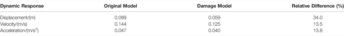
TABLE 5. Maximum dynamic response original model and damage model of simply supported beam.

3.2 Example of Truss Numerical Model

3.2.1 Calculated Value of Truss Displacement

The specific numerical model size of the truss structure is shown in Figure 9. The truss has 10 spans, 37 elements, which are all bar units, the length of the bottom and upper horizontal bar units is 0.4 m, 0.3 m for the vertical bar units, and 0.5 m for the diagonal bar units. The elastic modulus of the steel used is E = 200 GPa, the cross-sectional area of the L-shaped steel unit is A = 2.276 × 10⁻⁴ m², the density ρ = 7.8 × 10³ kg/m³, and the vertical concentrated force F = 15 kN is loaded at the bottom in the middle of the span.

FIGURE 9

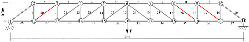
FIGURE 9. Sketch of truss model.

The unit stiffness matrix in the local coordinate system of the unit is expressed as

$K\text{e}=\frac{EA}{L}\left[\begin{array}{cc}1& \mathrm{-}1\\ \mathrm{-}1& 1\end{array}\right](25)$

where E is the elastic modulus of the unit, A is the cross-sectional area of the unit, and L is the length of the unit.

The transformation matrix of unit stiffness matrix in local coordinate system into that in global coordinate system can be expressed as

$S=\left[\begin{array}{cccc}\cos \theta & \sin \theta & 0& 0\\ 0& 0& \cos \theta & \sin \theta \end{array}\right](26)$

where θ is expressed as the rotation angle of the unit between the local coordinate system and the global coordinate system.

The given unit stiffness matrix and transformation matrix under the local coordinate system of the unit, the unit stiffness matrix under the local coordinate system can be transformed into the unit stiffness matrix under the global coordinate system, and the unit stiffness matrix $K_g^e$ (4 × 4 order matrix) under the global coordinate system can be obtained as follows:

$K_{\text{g}}^{\text{e}}=\frac{EA}{L}\left[\begin{array}{cccc}{\cos }^2\theta & \cos \theta \sin \theta & -{\cos }^2\theta & -\cos \theta \sin \theta \\ \cos \theta \sin \theta & {\sin }^2\theta & -\cos \theta \sin \theta & -{\sin }^2\theta \\ -{\cos }^2\theta & -\cos \theta \sin \theta & {\cos }^2\theta & \cos \theta \sin \theta \\ -\cos \theta \sin \theta & -{\sin }^2\theta & \cos \theta \sin \theta & {\sin }^2\theta \end{array}\right](27)$

In this example, the structure has 20 nodes with 40 degrees of freedom. The association table method (He et al., 2021; Huang and Schröder, 2021) requires an extraction matrix T_{4 × 40}. The matrix T extracts the degrees of freedom of different units in the global coordinate system. The T matrix changes with the degrees of freedom of unit and is expressed as

$T={\left[\begin{array}{cccccccccc}0& ···& 0& 1& 0& 0& 0& 0& ···& 0\\ 0& ···& 0& 0& 1& 0& 0& 0& ···& 0\\ 0& ···& 0& 0& 0& 1& 0& 0& ···& 0\\ 0& ···& 0& 0& 0& 0& 1& 0& ···& 0\end{array}\right]}_{4\times 40}(28)$

The unit stiffness matrix in the global coordinate system is

$K_{\text{g}}^E{=\text{T}}^{\text{T}}{K}_{\text{g}}^{\text{e}}T(29)$

where $K_g^E$ is 40 × 40 order matrix.

According to Equation 2 the damage coefficient ${\alpha }_i$ (0 < ${\alpha }_i$ < 1) is introduced, and the global stiffness matrix of the truss can be expressed as

$\mathit{K}={\displaystyle \sum _{i=1}^{37}\left(1-{\alpha }_i\right)}{\mathit{K}}_i(30)$

where K_i represents the $i-th$ unit stiffness matrix in the global coordinate system, and the subscript $i$ represents the unit number.

In order to obtain the static response of the structure, the vertical concentrated force F = 15 KN is loaded at the bottom in the middle of the span. The truss model is modeled by the correlation table method (He et al., 2021; Huang and Schröder, 2021). The steps of locating the position of the stiffness matrix by the correlation table method are as follows: assume that the node ($i$,j) of the unit N corresponds to the position of the node degrees of freedom of the global stiffness matrix as Ni(2×i-1, 2× $i$),Nj (2×j-1, 2×j). For example, for unit 12, the node numbers are 3 and 13, and the position of the node degrees of freedom corresponds to the global stiffness matrix are 5, 6, 25, and 26. Therefore, the corresponding positions of unit 12 in the global stiffness matrix are 5 rows, 6 rows, 25 rows, 26 rows, 5 columns, 6 columns, 25 columns, and 26 columns.

In order to better simulate the actual damage situation, different damage coefficient values are set for different units of the truss. Assuming that units 20, 26, and 27 are damaged by 15%, 60%, and 25%, that is, α₂₀ = 0.15, α₂₆ = 0.60, and α₂₇ = 0.25, Equation 3 can be used to solve the displacement values of each node after damage, as shown in Table 6. In the table, u and v represent horizontal and vertical displacements, respectively.

TABLE 6

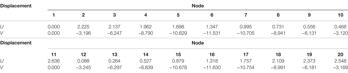
TABLE 6. Displacement values of unit nodes (mm).

Figure 10 shows the deformation diagram of the truss. In the figure, the dotted lines present the original structure, and the solid lines present the deformed structure.

FIGURE 10

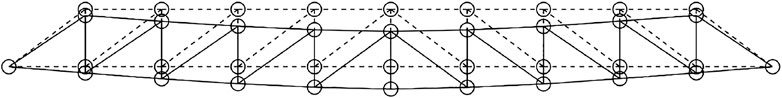
FIGURE 10. Deformation diagram of truss.

3.2.2 Truss Damage Identification

Table 6 can be used to calculate the node displacement value as the known value for structural damage identification.

According to Equation 5, the force residual vector P is obtained, which is listed in Table 7. In the table, $u_{\text{a}}$ and $v_{\text{a}}$ are the horizontal and vertical vectors of the premier node of the unit, respectively, while $u_{\text{b}}$ and $v_{\text{b}}$ are the horizontal and vertical vectors of the second node of the unit.

TABLE 7

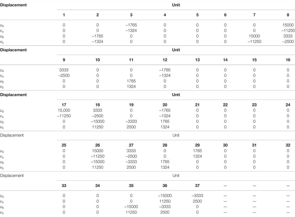
TABLE 7. Values of force residual vector P (N).

Figure 11 represents a distribution and arrangement diagram of the force residual vector P.

FIGURE 11

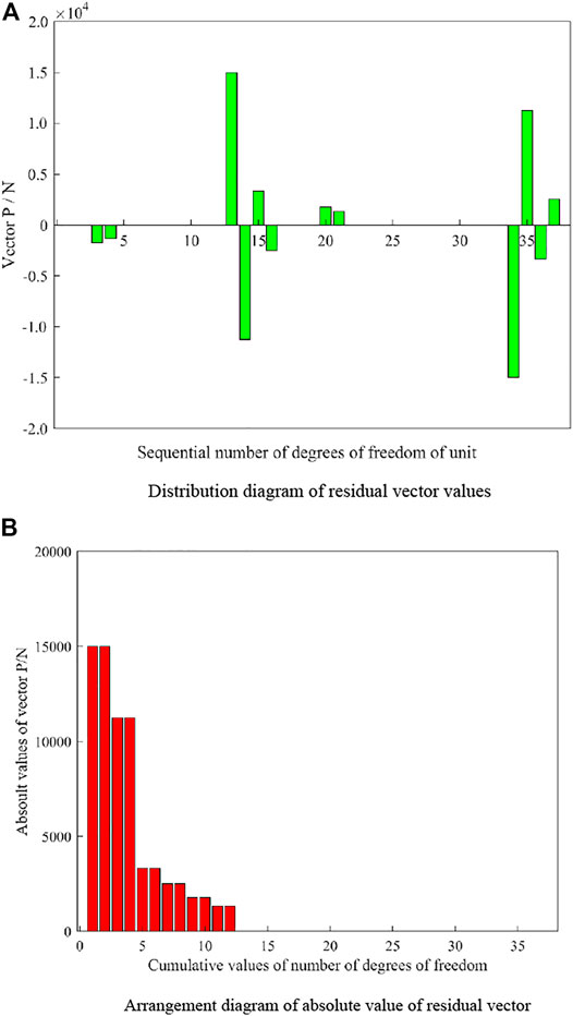
FIGURE 11. Distribution and arrangement of residual vector values of truss. (A) Distribution diagram of the residual vector values (B) Arrangement diagram of the absolute value of residual vector.

Figure 11A presents the distribution of force residual vector P. The abscissa represents the sequential number of the horizontal and vertical degrees of freedom of both nodes for each unit. The ordinate corresponds to the force residual vector of corresponding units. Figure 11B shows the arrangement of the absolute values of P in descending order. The abscissa represents the cumulative values of the number of the horizontal and vertical degrees of freedom of both nodes for each unit (the total number of degrees of freedom of unit nodes, including vertical degrees of freedom and corner degrees of freedom).

For the arranged absolute value sequence in Figure 11B, by dividing the previous element by the next element, we obtain the positioning diagram shown in Figure 12. The vertical coordinate of Figure 12 is expressed as the ratio of the absolute value P of the residual force vector corresponding to the first displacement and the third displacement in the element. The maximum ratio, which represents the total number of degrees of freedom of the damage units, is located at 12. Since each unit corresponds to 4 degrees of freedom in the local coordinate system, it can be seen that three units in the truss have been damaged, which is consistent with the set number of damaged units.

FIGURE 12

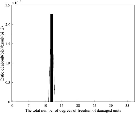
FIGURE 12. Total number of freedom degrees of damage units.

In Table 7, the truss units 20, 26, and 27, whose ratios of the residual stress vector value P corresponding to the first displacement and the third displacement of the element are -1, are the damaged units, and the damaged units located are the same as the set damaged units.

The identification values of damage degrees are obtained by solving damage degrees using Equation 6, and the setting values of the corresponding units are listed in Table 8.

TABLE 8

TABLE 8. Identification values and setting values of unit damage degrees of truss.

It can be seen from Table 8 that all the identification values of damage degrees are completely consistent with the corresponding setting values. It can be concluded that the force residual vector method can be used to locate the damage position and identify the damage degree of the truss structure.

Eraky et al. (2016), Abdo (2012) used the dynamic test method to obtain the eigenvalues and eigenvectors of the structure and combined it with the residual force vector method to identify the damage of the structure. In this article, the static displacement parameters are obtained by the static test method. The static displacement parameters are easier to obtain than the dynamic parameters, and the accuracy of the results is more accurate. In addition, this article uses the intelligent force residual vector algorithm to obtain more accurate results and faster damage identification.

3.2.3 Dynamic Response Analysis of Truss

Using the state space theory to simulate and analyze the dynamic response of the original truss model and damage model under the action of the El Centro seismic wave can verify the dynamic response degree of the structure under the seismic conditions of the original model and damage model, and predict whether the structure will be damaged under seismic load. Parameter setting of dynamic response analysis in this example: sampling frequency F_s = 50 Hz, sampling interval △t = 1/F_s = 0.01 s, number of generated samples N = 2500. Figure 13 shows the time history curve of El Centro seismic excitation applied to the model. Figure 14 shows the dynamic response of the displacement, velocity, and acceleration output of the original model of the truss. Figure 15 shows the dynamic responses of the displacement, velocity, and acceleration output of the damage model of the truss, and the peak value of the dynamic response in Figures 14 and 15 is the maximum value of the dynamic response of the displacement, velocity, and acceleration output.

FIGURE 13

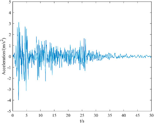
FIGURE 13. EL Centro seismic wave time history curve.

FIGURE 14

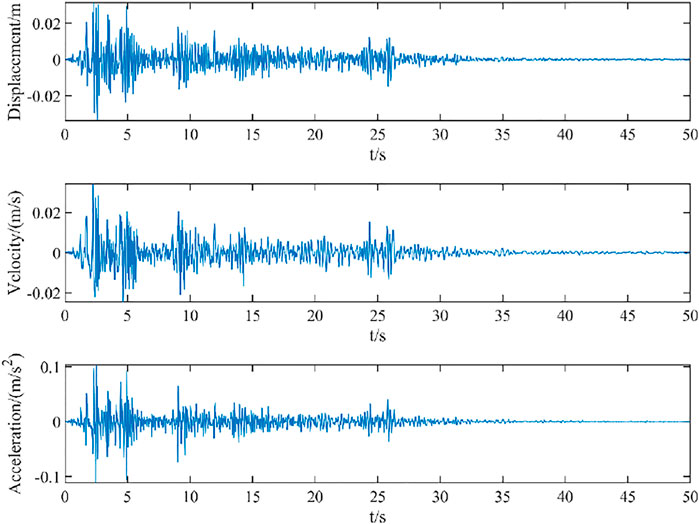
FIGURE 14. Dynamic response of displacement, velocity, and acceleration output of original truss model.

FIGURE 15

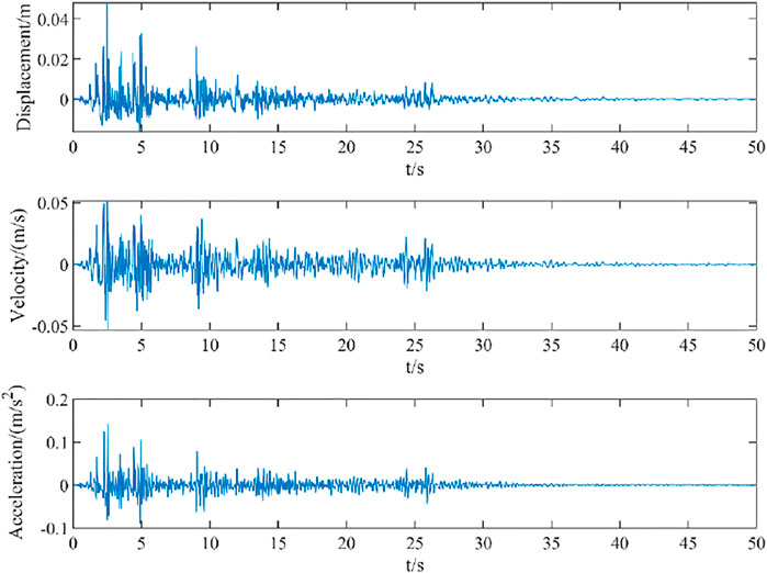
FIGURE 15. Dynamic response of displacement, velocity, and acceleration output of damage truss model.

It can be seen from Figure 14 that under the excitation of seismic wave, the displacement, velocity, and acceleration time history curve of the original model begins to decay freely around 2.50 s, the peak value of displacement is at 2.58 s, the peak value of velocity is at 2.22 s, and the peak value of acceleration is applied at 2.48 s. It can be seen from Figure 15 that under the excitation of seismic wave, the displacement, velocity, and acceleration time history curve of the original model begin to decay freely around 2.50 s, the peak value of displacement is at 2.46 s, the peak value of velocity is at 2.56 s, and the peak value of acceleration is at 2.52 s.

The extracted dynamic response peaks of displacement, velocity, and acceleration of the original model of truss and the damage model of truss are shown in Figures 14 and 15, and the relative difference between the dynamic response values of displacement, velocity, and acceleration of the original model and the damage model is calculated.

It can be seen from Table 9 that under the selected El Centro seismic wave excitation, the displacement response peak of the damage model exceeds the displacement response peak of the original model by 53.6%, the velocity response peak of the damage model exceeds the velocity response peak of the original model by 50.5%, and the acceleration response peak of the damage model exceeds the acceleration response peak of the original model by 38.1%. Considering the long-term use of the structure and the impact on the environment, the structural stiffness is bound to decay. The dynamic response analysis results of different stiffness models are quite different, which shows that the original model cannot effectively reflect the dynamic characteristics of the structure, so it is necessary to identify the damage of the original model. The model after damage identification under earthquake will not cause misjudgment of structural resistance, which further verifies the necessity of damage identification.

TABLE 9

TABLE 9. Maximum dynamic response original model and damage model of truss.

4 Conclusion

Based on the existing research results of the residual force vector method, a new structural damage identification method based on the force residual vector is proposed in this article. Through the identification analysis of some units of the simply supported beam numerical model and the truss numerical model under different damage degrees at the same time, it is shown that this method uses the arrangement of force residual vector elements to intelligently obtain the location of damage recognition, the number of damaged elements, and the degree of damage. It only needs the displacement information under static load and does not need complex modal analysis. In addition, because of the addition of substructure, the solution of the system will not be complicated; the damage identification result is faster, and the calculation speed has a great advantage.

The dynamic responses of the original model and the damaged truss model are simulated and compared by using the state space theory. Under the excitation of the El Centro seismic wave, the dynamic response peak of displacement, velocity, and acceleration of the damage model is much larger than that of the original model, and the original model cannot effectively reflect the dynamic characteristics of the structure. Therefore, it is necessary to identify the damage of the original model, and the model after damage identification will not have the problem of misjudgment of structural resistance under seismic excitation. It can better reflect the potential safety hazards caused by excessive amplitude, velocity, and acceleration of the actual structure under seismic dynamic excitation.

Data Availability Statement

The original contributions presented in the study are included in the article/Supplementary Material; further inquiries can be directed to the corresponding author.

Author Contributions

JS: designed research schemes and drafted and revised the manuscript. ZL: drafted and revised the manuscript. SL: put forward research ideas and revised the manuscript. WW: thesis revision and research funding support.

Conflict of Interest

The authors declare that the research was conducted in the absence of any commercial or financial relationships that could be construed as a potential conflict of interest.

Publisher’s Note

All claims expressed in this article are solely those of the authors and do not necessarily represent those of their affiliated organizations, or those of the publisher, the editors, and the reviewers. Any product that may be evaluated in this article, or claim that may be made by its manufacturer, is not guaranteed or endorsed by the publisher.

References

Abdo, M. A.-B., and Hori, M. (2002). A Numerical Study of Structural Damage Detection Using Changes in the Rotation of Mode Shapes. J. Sound Vib. 251, 227–239. doi:10.1006/jsvi.2001.3989

CrossRef Full Text | Google Scholar

Abdo, M. A.-B. (2012). Parametric Study of Using Only Static Response in Structural Damage Detection. Eng. Struct. 34, 124–131. doi:10.1016/j.engstruct.2011.09.027

CrossRef Full Text | Google Scholar

Azim, M. R., and Gül, M. (2021). Data-driven Damage Identification Technique for Steel Truss Railroad Bridges Utilizing Principal Component Analysis of Strain Response[J]. Struct. Infrastructure Eng. 17 (8), 1019–1035. doi:10.1080/15732479.2020.1785512

CrossRef Full Text | Google Scholar

Cornwell, P., Doebling, S. W., and Farrar, C. R. (1999). Application of the Strain Energy Damage Detection Method to Plate-like Structures. J. Sound Vib. 224, 359–374. doi:10.1006/jsvi.1999.2163

CrossRef Full Text | Google Scholar

Debruyne, S., Vandepitte, D., and Moens, D. (2015). Identification of Design Parameter Variability of Honeycomb Sandwich Beams from a Study of Limited Available Experimental Dynamic Structural Response Data. Comput. Struct. 146, 197–213. doi:10.1016/j.compstruc.2013.09.004

CrossRef Full Text | Google Scholar

Di Paola, M., and Bilello, C. (2004). An Integral Equation for Damage Identification of Euler-Bernoulli Beams under Static Loads. J. Eng. Mech. 130, 225–234. doi:10.1061/(asce)0733-9399(2004)130:2(225)

CrossRef Full Text | Google Scholar

Eftekhar Azam, S., Rageh, A., and Linzell, D. (2019). Damage Detection in Structural Systems Utilizing Artificial Neural Networks and Proper Orthogonal Decomposition. Struct. Control Health Monit. 26 (2), e2288. doi:10.1002/stc.2288

CrossRef Full Text | Google Scholar

Emmert, T., Meindl, M., Jaensch, S., and Polifke, W. (2016). Linear State Space Interconnect Modeling of Acoustic Systems. Acta Acustica united Acustica 102 (5), 824–833. doi:10.3813/aaa.918997

CrossRef Full Text | Google Scholar

Eraky, A., Saad, A., Anwar, A. M., and Abdo, A. (2016). Damage Detection of Plate-like Structures Based on Residual Force Vector. HBRC J. 12 (3), 255–262. doi:10.1016/j.hbrcj.2015.01.005

CrossRef Full Text | Google Scholar

Eun-Taik, L., and Hee-Chang, E. (2018). Damage Identification by the Data Expansion and Substructuring Methods[J]. Adv. Civ. Eng. 12. doi:10.1155/2018/1867562

CrossRef Full Text | Google Scholar

Gomes, G. F., de Almeida, F. A., Junqueira, D. M., da Cunha, S. S., and Ancelotti, A. C. (2019). Optimized Damage Identification in CFRP Plates by Reduced Mode Shapes and GA-ANN Methods. Eng. Struct. 181, 111–123. doi:10.1016/j.engstruct.2018.11.081

CrossRef Full Text | Google Scholar

Han, D. Y., Luo, H., and Kong, X. X. (2021). Damage Identification of a Derrick Steel Structure Based on the Transient Energy Curvature of HVD Envelope Spectrum [J]. J. Vib. Shock 40 (02), 135–140. doi:10.13456/j.cnki.jvs.2021.02.018

CrossRef Full Text | Google Scholar

Han, D. Y., and Shi, P. M. (2012). Identification of Derrick Steel Structures Damage Based on Frequency and BP Neural Network [J]. China Saf. Sci. J. 22 (08), 118–123. doi:10.16265/j.cnki.issn1003-3033.2012.08.010

CrossRef Full Text | Google Scholar

He, H., Zheng, J., Liao, L., and Chen, Y. J. (2021). Damage Identification Based on Convolutional Neural Network and Recurrence Graph for Beam Bridge[J]. Struct. Health Monit. 20 (4), 1392–1408. doi:10.1177/1475921720916928

CrossRef Full Text | Google Scholar

Huang, M., Cheng, S., Zhang, H., Gul, M., and Lu, H. (2019). Structural Damage Identification under Temperature Variations Based on PSO-CS Hybrid Algorithm. Int. J. Str. Stab. Dyn. 19 (11), 1950139. doi:10.1142/s0219455419501396

CrossRef Full Text | Google Scholar

Huang, T., and Schröder, K.-U. (2021). A Bayesian Probabilistic Approach for Damage Identification in Plate Structures Using Responses at Vibration Nodes. Mech. Syst. Signal Process. 146, 106998. doi:10.1016/j.ymssp.2020.106998

CrossRef Full Text | Google Scholar

Huynh, D., He, J., and Tran, D. (2005). Damage Location Vector: A Non-destructive Structural Damage Detection Technique. Comput. Struct. 83, 2353–2367. doi:10.1016/j.compstruc.2005.03.029

CrossRef Full Text | Google Scholar

Kahl, K., and Sirkis, J. S. (1996). Damage Detection in Beam Structures Using Subspace Rotation Algorithm with Strain Data. AIAA J. 34 (12), 2609–2614. doi:10.2514/3.13446

CrossRef Full Text | Google Scholar

Kasper, D. G., Swanson, D. C., and Reichard, K. M. (2008). Higher-frequency Wavenumber Shift and Frequency Shift in a Cracked, Vibrating Beam. J. Sound Vib. 312, 1–18. doi:10.1016/j.jsv.2007.07.092

CrossRef Full Text | Google Scholar

Kirsch, U. (2003). Approximate Vibration Reanalysis of Structures. AIAA J. 41 (3), 504–511. doi:10.2514/2.1973

CrossRef Full Text | Google Scholar

Li, H., Lu, Z., and Liu, J. (2016). Structural Damage Identification Based on Residual Force Vector and Response Sensitivity Analysis. J. Vib. Control 22 (11), 2759–2770. doi:10.1177/1077546314549822

CrossRef Full Text | Google Scholar

Link, R. J., and Zimmerman, D. C. (2015). Structural Damage Diagnosis Using Frequency Response Functions and Orthogonal Matching Pursuit: Theoretical Development. Struct. Control Health Monit. 22, 889–902. doi:10.1002/stc.1720

CrossRef Full Text | Google Scholar

Mousavi, A. A., Zhang, C., Masri, S. F., and Gholipour, G. (2021). Damage Detection and Localization of a Steel Truss Bridge Model Subjected to Impact and White Noise Excitations Using Empirical Wavelet Transform Neural Network Approach. Measurement 185, 110060. doi:10.1016/j.measurement.2021.110060

CrossRef Full Text | Google Scholar

Nguyen, K.-D., Chan, T. H., and Thambiratnam, D. P. (2016). Structural Damage Identification Based on Change in Geometric Modal Strain Energy-Eigenvalue Ratio. Smart Mat. Struct. 25 (7), 075032. doi:10.1088/0964-1726/25/7/075032

CrossRef Full Text | Google Scholar

Nobahari, M., Ghasemi, M. R., and Shabakhty, N. (2018). A Fast and Robust Method for Damage Detection of Truss Structures[J]. Appl. Math. Model. 68, 368–382. doi:10.1016/j.apm.2018.11.025

CrossRef Full Text | Google Scholar

Nogal, M., Lozano-Galant, J. A., Turmo, J., and Castillo, E. (2016). Numerical Damage Identification of Structures by Observability Techniques Based on Static Loading Tests. Struct. Infrastructure Eng. 12 (9), 1216–1227. doi:10.1080/15732479.2015.1101143

CrossRef Full Text | Google Scholar

OBrien, E. J., and Malekjafarian, A. (2016). A Mode Shape-Based Damage Detection Approach Using Laser Measurement from a Vehicle Crossing a Simply Supported Bridge. Struct. Control Health Monit. 23 (10), 1273–1286. doi:10.1002/stc.1841

CrossRef Full Text | Google Scholar

Pérez, M. A., and Serra-López, R. (2019). A Frequency Domain-Based Correlation Approach for Structural Assessment and Damage Identification[J]. Mech. Syst. Signal Process. 119, 432–456. doi:10.1016/j.ymssp.2018.09.042

CrossRef Full Text | Google Scholar

Rangapuram, S. S., Seeger, M. W., Gasthaus, J., Stella, L., Wang, Y. Y., and Januschowski, T. (2018). Deep State Space Models for Time Series Forecasting[J]. Adv. neural Inf. Process. Syst., 31.

Google Scholar

Rucevskis, S., Janeliukstis, R., Akishin, P., and Chate, A. (2016). Mode Shape-Based Damage Detection in Plate Structure without Baseline Data. Struct. Control Health Monit. 23 (9), 1180–1193. doi:10.1002/stc.1838

CrossRef Full Text | Google Scholar

Shi, P. M., Yin, X. D., Han, D. Y., and Luo, H. (2020). Study on Damage Identification Method of Steel Structure Based on Relative Curvature of HVD Marginal Spectral Entropy [J]. Mod. Manuf. Eng. (12), 136–142. doi:10.16731/j.cnki.1671-3122.2020.12.022

CrossRef Full Text | Google Scholar

Silva, C. F., Pettersson, P., Iaccarino, G., and Ihme, M. (2020). Uncertainty Quantification of Combustion Noise by Generalized Polynomial Chaos and State-Space Models. Combust. Flame 217, 113–130. doi:10.1016/j.combustflame.2020.03.010

CrossRef Full Text | Google Scholar

Sung, S. H., Jung, H. J., and Jung, H. Y. (2013). Damage Detection for Beam-like Structures Using the Normalized Curvature of a Uniform Load Surface. J. Sound Vib. 332, 1501–1519. doi:10.1016/j.jsv.2012.11.016

CrossRef Full Text | Google Scholar

Truong, T. T., Dinh-Cong, D., Lee, J., and Nguyen-Thoi, T. (2020). An Effective Deep Feedforward Neural Networks (DFNN) Method for Damage Identification of Truss Structures Using Noisy Incomplete Modal Data. J. Build. Eng. 30, 101244. doi:10.1016/j.jobe.2020.101244

CrossRef Full Text | Google Scholar

Varanasi, S. K., and Jampana, P. (2020). Nuclear Norm Subspace Identification of Continuous Time State-Space Models with Missing Outputs. Control Eng. Pract. 95, 104239. doi:10.1016/j.conengprac.2019.104239

CrossRef Full Text | Google Scholar

Wang, Y., Thambiratnam, D. P., Chan, T. H. T., and Nguyen, A. (2018). Damage Detection in Asymmetric Buildings Using Vibration-Based Techniques. Struct. Control Health Monit. 25 (5), e2148. doi:10.1002/stc.2148

CrossRef Full Text | Google Scholar

Wei Fan, W., and Pizhong Qiao, P. Z. (2011). Vibration-based Damage Identification Methods: A Review and Comparative Study. Struct. Health Monit. 10, 83–111. doi:10.1177/1475921710365419

CrossRef Full Text | Google Scholar

Zhan, J., Zhang, F., Siahkouhi, M., Kong, X., and Xia, H. (2021). A Damage Identification Method for Connections of Adjacent Box-Beam Bridges Using Vehicle-Bridge Interaction Analysis and Model Updating. Eng. Struct. 228, 111551. doi:10.1016/j.engstruct.2020.111551

CrossRef Full Text | Google Scholar

Zhang, W., Wang, Z., and Ma, H. (2009). Crack Identification in Stepped Cantilever Beam Combining Wavelet Analysis with Transform Matrix. Acta Mech. Solida Sin. 22 (4), 360–368. doi:10.1016/s0894-9166(09)60285-8

CrossRef Full Text | Google Scholar

Zhuo, D., and Cao, H. (2021). Damage Identification of Bolt Connection in Steel Truss Structures by Using Sound Signals. Struct. Health Monit. 21 (2), 501–517. doi:10.1177/14759217211004823

CrossRef Full Text | Google Scholar

Zimmerman, D. C., and Kaouk, M. (1992). Structural Damage Detection in Beam Structures Using a Subspace Rotation Algorithm [J]. AIAA J. 34 (12), 2341–2350.

Google Scholar