Machine learning-accelerated small-angle X-ray scattering analysis of disordered two- and three-phase materials

1 Introduction

For heterogeneous, disordered materials, the microstructure i.e. the geometry of the different phases substantially influences the performance of a material, e.g., thermal, electric, mechanical, and mass transport properties (Torquato, 2010). Therefore, characterizing the microstructure is a crucial step towards understanding the material and optimizing its design. A vast number of applications of advanced materials rely on precise control of physical and chemical processes within a microstructure with length scales in the nanometer range, like batteries, chemical separation techniques, and chromatography (Gommes, 2018). To characterize detailed random porous structures, high-resolution 3D imaging techniques e.g., micro/nano X-ray computed tomography (X-ray CT), focused ion beam scanning electron microscopy (FIB-SEM), and transmission electron microscopy tomography (TEMT) can provide high quality information on morphological features. Nevertheless, imaging techniques are frequently time-consuming and require advanced sample preparation methods or sample environments. Moreover, the attainable contrast is strongly sample-dependent and can be prohibitively low.

Complementary to imaging approaches at the nanoscale, small-angle X-ray scattering (SAXS) is a powerful technique that characterizes the nanostructure via a scattering intensity measured in the spectral domain (reciprocal space). More precisely, the spatial distribution of electron density is indirectly observed through the elastic scattering behaviour of X-rays passing through the material. The interaction with the sample forces the X-rays to change direction with a certain angle (the scattering angle). The intensity as a function of scattering angle is related to the electron density distribution through a Fourier transform. With a modern 2D pixel-array detector, SAXS can easily provide structural information for sub-micron length scales and all the way down to a few Ångström, by changing the sample-to-detector distance from meters to millimeters accordingly. In addition, owing to the high penetration power of X-rays, the sample can be studied in different states of matter e.g. gas, solution, or solid, and in other conditions coupled with thermal, mechanical, electrical and magnetic fields (Li et al., 2016). With the latest X-ray detection techniques, SAXS measurements become rather fast, in particular at synchrotron facilities offering high photon flux where hundreds of measurements per second can be performed. This enables so-called in situ/in-operando characterization of continuous nanostructure development. SAXS has been applied to numerous types of materials including nanostructures (Li et al., 2016), biomacromolecules (Blanchet and Svergun, 2013), polymers (Chu and Hsiao, 2001), and porous materials (Welborn and Detsi, 2020).

However, a major challenge of SAXS is that the electron density distribution is in general not uniquely determined by the scattering intensity, owing to the ‘phase problem’ (Taylor, 2003): as X-rays are electromagnetic waves having two important parameters, amplitude and phase, the intensity recorded on the detector is the modulus of the wave’s Poynting vector and proportional to the square of the amplitude of the scattered wave, while the phase information is lost in the experiment. In addition, for isotropic systems, the scattering intensity can be presented in a one-dimensional curve that constitutes spherically-averaged spectral magnitudes, further compressing the information. In effect, the SAXS data contains much less information than the corresponding full, three-dimensional Fourier transform. Limited prior knowledge warrants the fitting of multiple SAXS models in a trial-and-error fashion, which can be a daunting task even for an experienced investigator (Archibald et al., 2020; Do et al., 2020). Further, fitting of non-analytical models can be computationally prohibitive.

Because data analysis constitutes a bottleneck in the use of SAXS, numerous approaches based on machine learning have been proposed in recent years, with the aim of accelerating the data analysis and providing decision support for the operator. Most also focus on biomacromolecules and nanoparticles, which are usually characterized in dilute solution by SAXS. For example, Franke et al. (Franke et al., 2018) use k-nearest neighbors to classify SAXS data based on particle shapes, diameters, and molecular mass; Archibald et al. (Archibald et al., 2020) use weighted k-nearest neighbors and Gaussian processes for classifying SAXS data and determine the most probable type of structure; He et al. (He et al., 2020) use a convolutional neural network-based autoencoder combined with a genetic algorithm to search for structures that are consistent with SAXS data; Scherdel et al. (Scherdel et al., 2021) use machine learning to directly predict effective properties such as thermal conductivity of silica aerogels; Tomaszewski et al. (Tomaszewski et al., 2021) evaluate numerous machine learning approaches to classifying SAXS data.

In this work, we investigate disordered, porous materials where the electron density distribution is modeled using thresholded Gaussian Random Fields (GRFs). This serves as a model system representing continuous multiphase distributions with irregular geometric shapes; this is different from many biomacromolecules and nanoparticles characterized by SAXS which are often treated as isolated systems and can be modelled ab initio. GRFs are frequently used as models for materials microstructures, because they realistically describe phase-separated, heterogeneous materials, originating from a description of spinodal decomposition by Cahn and Hilliard (Cahn and Hilliard, 1958). GRFs have been used in models for scattering data (Berk, 1991; Quintanilla et al., 2007; Gommes, 2013; Gommes and Roberts, 2018) and as material models for a wide variety of materials both for SAXS analysis and otherwise, including microemulsions (Teubner, 1991; Chen et al., 1996), polymer blends (Jinnai et al., 1997; D’hollander et al., 2010; Barman et al., 2019), lithium-ion batteries (Feinauer et al., 2015), porous alloys for energy storage and catalysis (Geslin et al., 2015; Lu et al., 2018), and gels (Roberts, 1997; Gommes and Roberts, 2008). We study the case of two phases, pore (vacuum/air) and solid, and three phases, where the third phase is an intermediate layer residing by the interface between pore and solid. We generate a large number of virtual microstructures for a number of cases. We further develop a Fourier transform-based numerical method for simulating realistic SAXS data. Both the structure generation and SAXS simulation methods are heavily optimized and implemented on GPU with a combined execution time in the order of 1 s. Using the simulated SAXS data as input and the known generation parameters as target output in a machine learning framework, we demonstrate that length scales and volume fractions can be predicted with good accuracy. Our framework is a proof of concept that can be applied to other types of disordered materials as well, in particular other Gaussian random field-based models with different covariance structures.

2 Results and discussion

2.1 Simulation of scattering intensity

In SAXS, the sample is irradiated with collimated or focused X-rays, the incident-radiation wavelength (of the monochromatic X-rays) being λ. The intensity of the elastically scattered X-ray is measured as a function of the magnitude of the scattering vector, q = |q|, where $\mathbf{q}=2\pi \left(\mathbf{k}-{\mathbf{k}}_{\mathbf{0}}\right)$. Here, k₀ and k are the wave vectors of the X-rays before and after scattering. The scattering angle 2θ is related to q by q = 4π sin(θ)/λ (Sorbier et al., 2019). Since the scattering arises from the interaction between X-rays and the electron clouds of the atoms, theoretically the scattering intensity can be written as

$I\left(\mathbf{q}\right)=|\left(\mathcal{F}\rho \right)\left(\mathbf{q}\right){|}^2,(1)$

where $\mathcal{F}\rho$ is the (3D) Fourier transform of the electron density. In practice, the theoretic intensity may be compared to the experimental data with a prefactor I₀ which depends on experimental conditions, and is not considered in this work by assuming that I₀ = 1 throughout. The 1D scattering data is acquired as a spherical mean intensity in q space, I(q), computed by orientational averaging over the spherical shell formed by all q with magnitude q (Schmidt-Rohr, 2007). The SAXS curve consists of measured values of I(q) for a large number of typically equidistant q values in the range q_min ≤ q ≤ q_max.

Assume that a virtual electron density ρ is simulated on a periodic cubic domain, i.e. a 3D voxel array, with resolution N³ and voxel size Δx. Then the fast Fourier transform (FFT) can be used to obtain the discrete counterpart to the scattering intensity, which we again denote by I(q). It is also defined on a periodic cubic domain with resolution N³, for all ${\mathbf{q}}_{\mathit{ijk}}=\left(q_x^{(i)},q_y^{(j)},q_z^{(k)}\right)$ such that

$q_x^{\left(i\right)}=\frac{2\pi }{N\mathrm{\Delta }x}i(2)$

for i = −N/2, − N/2 + 1, … , N/2–2, N/2–1, and likewise for $q_y^{(j)}$ and $q_z^{(k)}$. An orientation-averaged scattering intensity I(q) (an “intensity data reduction”) can then be computed as

$I\left(q\right)=\sum _{i,j,k}{w}_q\left({\mathbf{q}}_{\mathit{ijk}}\right)I\left({\mathbf{q}}_{\mathit{ijk}}\right),(3)$

where w_q is a weight function such that

$w_q\left({\mathbf{q}}_{\mathit{ijk}}\right)=\frac{w_{q,0}}{q_{\mathit{ijk}}^2}\exp \left[-2{\left(\frac{q_{\mathit{ijk}}-q}{\mathrm{\Delta }q}\right)}^2\right](4)$

for q_ijk = |q_ijk|, Δq = 2π/(NΔx) (the grid resolution in q space), with $w_q\left(\mathbf{0}\right)=0$ and w_q,0 chosen so that the sum of the weights is 1. Effectively, w_q describes a normal distribution in the radial direction with mean q and standard deviation Δq/2, all weights rescaled with $1/q_{\mathit{ijk}}^2$ to compensate for the fact that the number of grid points increases in proportion to $4\pi q_{\mathit{ijk}}^2$ (the area of a spherical shell with radius q_ijk).

In practice, because of the symmetries in q space, the N³ array I(q) can be folded into a (N/2 + 1)³ array which substantially reduces the computation time (for the steps corresponding to Eqs 3, 4). The simulation is implemented on GPU in Matlab (Mathworks, Natick, MA, US).

2.2 Microstructure model

In the original model by Cahn and Hilliard (Cahn and Hilliard, 1958), GRFs arose as a solution to a spinodal decomposition model described as a superposition of cosine waves,

$\psi \left(\mathbf{x}\right)=\sqrt{\frac{2}{M}}\sum _{m=1}^M\cos \left({\mathbf{q}}_m\cdot \mathbf{x}+{\eta }_m\right),(5)$

for M ≫ 1, some wave vectors q_m and random phase offsets η_m, 0 ≤ η_m < 2π. The wave vectors follow some probability distribution $\mathrm{\Gamma }\left(\mathbf{q}\right)$; if it is radially symmetric and only a function of |q|, the GRF is statistically isotropic. A disadvantage of constructing a GRF like this is that ψ(x) is not a periodic function unless the wave vectors are constrained to axis-aligned directions and certain magnitudes.

Therefore, we instead use a method based on the Fast Fourier Transform (FFT) (Lang and Potthoff, 2011). A GRF can generally be described by a mean value and a covariance function (Liu et al., 2019). The spectral density of this covariance function actually equals $\mathrm{\Gamma }\left(\mathbf{q}\right)$ (Teubner, 1991). Generating a GRF in a cubic domain with resolution N³ is performed as follows. Gaussian noise is generated in the spatial domain. Then, it is Fourier transformed and multiplied by the square root of the spectral density of the target covariance function. Finally, the result is inverse Fourier transformed, yielding a GRF ψ(x) with the specified covariance function. In other words, starting with Gaussian white noise W(x), where W is $\mathcal{N}(\mathrm{0,1})$-distributed and independent for all x, the GRF is obtained as

$\psi \left(\mathbf{x}\right)=\left({\mathcal{F}}^{-1}{\mathrm{\Gamma }}^{1/2}\mathcal{F}W\right)\left(\mathbf{x}\right)(6)$

We use the spectral density

$\mathrm{\Gamma }\left(\mathbf{q}\right)={\left(1+|a\mathbf{q}{|}^8\right)}^{-2},(7)$

a special case of a spectral density used before (Matérn, 1986; Lang and Potthoff, 2011), also in models for materials microstructures (Röding et al., 2020; Prifling et al., 2021) (note that the spectral density is not normalized hence not a probability distribution; this only results in a linear scaling of the GRF, which is of no concern here). Because $\mathcal{F}W$ and Γ are both symmetric, ψ(x) is real-valued. The parameter a has dimension length and we refer to it as a scaling parameter, to which the length scale is approximately proportional. It is important to note that the length scale is determined not only by a but by the entire functional form of Γ.

We model both two phases, pore (vacuum/air) and solid, and three phases, where the third phase is an intermediate layer residing by the interface between pore and solid. The layer can be regarded as a material condensed at the surface of the solid phase. The microstructures are parameterized by the scaling parameter a, the porosity ϵ, and the fraction ν of the pore space filled up by the intermediate layer; for the two-phase microstructures, ν = 0. The volume fractions are ϵ(1 − ν), ϵν, and 1 − ϵ for pore, layer, and solid. In addition, electron densities need to be specified. We let all electron densities be between 0 (vacuum) and one for convenience; the scattering intensity is proportional to the mean squared fluctuation of the electron density of the material (Welborn and Detsi, 2020) but also to other experimental factors such as X-ray photon flux. Therefore, the scattering intensity can always be rescaled. We choose ρ_pore = 0, ρ_layer = 0.65, and ρ_solid = 1. Assuming that the intermediate layer is water, the electron density ratio between the layer and the solid phase is fairly close to that of water to cellulose (density 1.5 g/cm³, ρ_layer ≈ 0.69), and water to hard carbon (Nishi and Pistoia, 2014) (density 1.45–1.55 g/cm³, ρ_layer ≈ 0.69–0.74), all of which were estimated by using refractive index at around 8 keV (Cu K-alpha X-ray source) from the center of X-ray optics (Henke et al., 1993).

Microstructures are generated from the GRFs in the following manner. First, a binary function is obtained by thresholding,

${\psi }^{\prime }\left(\mathbf{x}\right)=\left\{\begin{array}{cc}0,\hfill & \psi \left(\mathbf{x}\right)\le T\hfill \\ 1,\hfill & \psi \left(\mathbf{x}\right)>T\hfill \end{array}\right.,(8)$

for T such that p (ψ(x) ≤ T) = ϵ. Second, ψ′ is smoothed with a 3D Gaussian filter (accounting for periodicity; σ = 2 voxels, but this choice is not crucial), yielding ψ″, 0 ≤ ψ″ ≤ 1. Two-phase electron densities can now be defined by

$\rho \left(\mathbf{x}\right)=\left\{\begin{array}{cc}{\rho }_1,\hfill & {\psi }^{″}\left(\mathbf{x}\right)\le T\hfill \\ {\rho }_2,\hfill & {\psi }^{″}\left(\mathbf{x}\right)>T\hfill \end{array}\right.(9)$

for T such that p (ψ″(x) ≤ T) = ϵ. Three-phase electron densities can be defined similarly by

$\rho \left(\mathbf{x}\right)=\left\{\begin{array}{cc}{\rho }_1,\hfill & {\psi }^{″}\left(\mathbf{x}\right)\le T_1\hfill \\ {\rho }_2,\hfill & T_1<{\psi }^{″}\left(\mathbf{x}\right)\le T_2\hfill \\ {\rho }_3,\hfill & {\psi }^{″}\left(\mathbf{x}\right)>T_2\hfill \end{array}\right.(10)$

for T₁ such that p (ψ″(x) ≤ T₁) = ϵ(1 − ν) and T₂ such that p (T₁ < ψ″(x) ≤ T₂) = ϵν) (and also p (ψ″(x) > T₂) = 1 − ϵ)).

Note that the ‘intermediate’ values of ψ″ (not equal to 0 or 1) will be concentrated near what will be the pore-solid interface, which is the reason for defining it this way. It ensures that with high probability, the intermediate layer will be adjacent to both pore and solid. If, on the other hand, ρ(x) would be obtained by thresholding ψ(x) directly, parts of the intermediate layer phase might end up in contact only with pore or only with solid in all directions, which would not be physically plausible. It is also worth pointing out that by using the 3D Gaussian filter also in the two-phase model, the two- and three-phase models are seamlessly integrated into the same framework and the two-phase model is a special case of the three-phase model.

The generation procedure is illustrated with microstructures generated on a grid of size 512³ with voxel size Δx = 0.5 nm (therefore the parameter a also has unit nm). In Figure 1, using a single 2D slice of a three-phase model with a = 4 nm, ϵ = 0.60, and ν = 0.50. In Figure 2, a 3D visualization of the same structure is shown. The simulation is implemented on GPU in Matlab (Mathworks, Natick, MA, US).

FIGURE 1

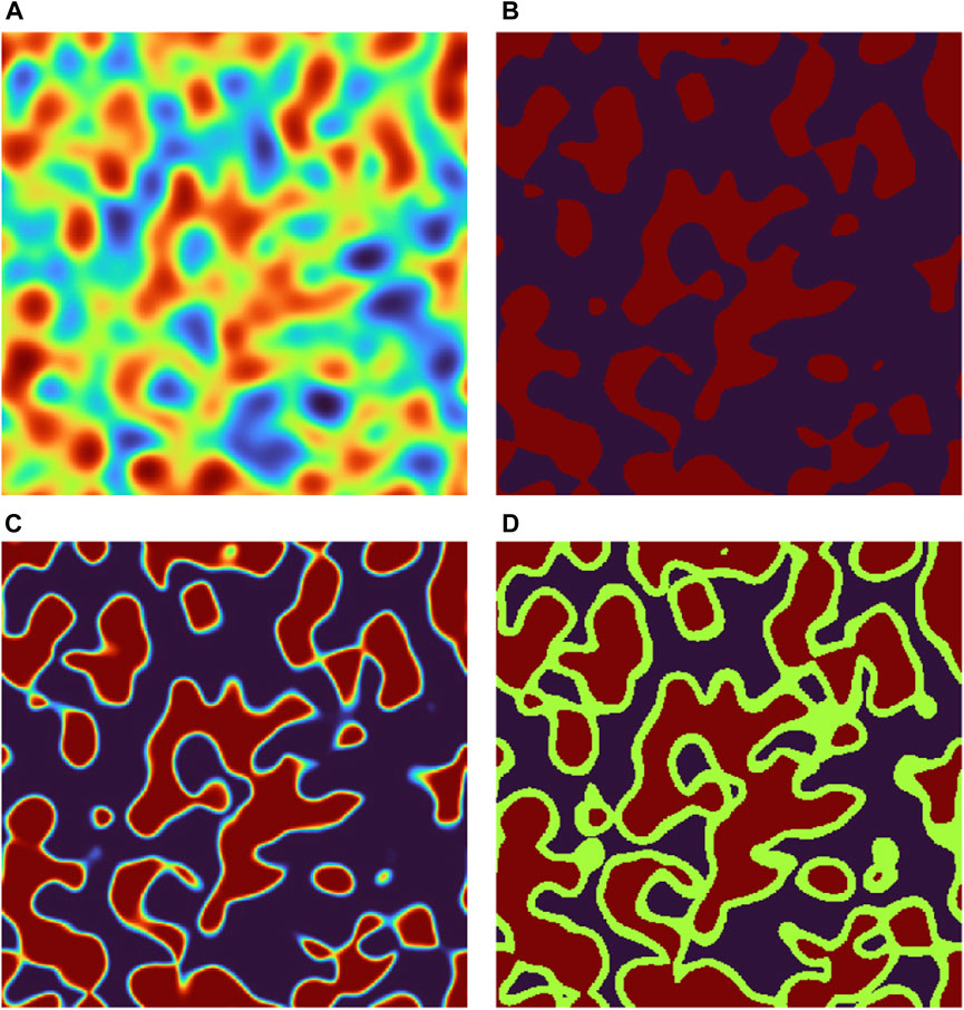
FIGURE 1. Illustration of a single 2D slice of a three-phase model with a =4 nm, ϵ =0.60, and ν =0.50. In (A), the GRF is shown (arbitrary intensity scale). In (B), a binary structure is shown, obtained from (A) by thresholding at the quantile ϵ. In (C), a smooth structure is shown, obtained from (B) by smoothing with a 3D Gaussian filter. In (D), the final electron density is shown, obtained from (C) by thresholding at the quantiles ϵ(1− ν) and ϵ.

FIGURE 2

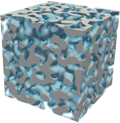
FIGURE 2. Illustration of a three-phase model with a =4 nm, ϵ =0.60, and ν =0.50. For an illustration of a single 2D slice from this model, see Figure 1.

2.3 Dataset generation

For developing a machine learning-based model for prediction of microstructural parameters, a large number of microstructures are generated on a grid of size 512³ with voxel size Δx = 0.5 nm (we reiterate that therefore the parameter a also has unit nm, whereas ϵ and ν are dimensionless quantities).

We reiterate that two-phase microstructures are generated using ρ_pore = 0 and ρ_solid = 1; varying ρ_solid is unnecessary because SAXS data can always be rescaled. Three-phase microstructures are generated using the same values and additionally ρ_layer = 0.65.

For all datasets, the scaling parameter a is uniformly distributed in [0.8, 8] nm. The resulting range of length scales is found to be represented well considering the resolution and simulation box size and to be accessible in the simulated q range. We generate four separate datasets: 1) two-phase, low porosity structures 2) two-phase, high porosity structures, 3) three-phase, low porosity structures, and 4) three-phase, high porosity structures. The porosity ϵ is uniformly distributed in [0.1, 0.5] for the low porosity structures and in [0.5, 0.9] for the high porosity structures. For the three-phase structures, the fraction of the intermediate layer in the pores ν is uniformly distributed in [0.05, 0.5] in both cases. The reason why porosities lower and higher than 0.5 are treated separately is that in the two-phase case, the values ϵ and 1 − ϵ literally cannot be distinguished because they are ‘mirror images’ of each other; therefore, approximate information about the porosity needs to be supplied as an input from e.g. sample contrast. This symmetry is referred to as Babinet’s principle and is reflected in the so-called Porod invariant of a two-phase scattering pattern (Zhang et al., 2012),

$Q={\int }_0^{\infty }I\left(q\right)q^2\mathrm{d}q\propto 2\pi \mathrm{\Delta }{\rho }^2ϵ\left(1-ϵ\right),(11)$

where Δρ is the electron density difference between the two phases, which is one in our case. So, whether the structure has low or high porosity is information that has to be supplied by the user. In the three-phase case, the situation is more complex, and unless ρ_layer = 1/2 there is no exact mirror image. Nevertheless, we treat two- and three-phase structures consistently in this respect.

For each of the four cases, 2¹⁹ (524,288) microstructures are generated for the training dataset, 2¹⁸ (262,144) for the validation dataset, and 2¹⁷ (131,072) for the test dataset. The scattering intensity is simulated for 500 q values, equidistant between q_min ≈ 0.04 nm⁻¹ and q_max ≈ 3.00 nm⁻¹; these values are taken from an in-house experimental setup using an Anton Paar SAXSpoint 2.0 (Anton Paar, Graz, Austria) and cover a normal SAXS probing range without losing the generality. On an NVIDIA A40 GPU, the average execution time for microstructure generation and simulation of SAXS data combined is approximately 1 s.

Note that the simulation of the scattering intensity I(q) described above does not account for measurement noise. The specifics of the noise are dependent on the experimental conditions (such as photon flux and quantum efficiency of the detector) and thereby on the intensity scale determined by the unknown prefactor I₀, as aforementioned. We use a noise model inspired by the Poisson distributed photon counting nature of the data acquisition (Sedlak et al., 2017). A Poisson model would imply that the variance of the noise is σ²(q) = I(q); however, considering the intensity scales resulting from using I₀ = 1, this model assumption does not produce realistic noise levels. Instead, we use a lognormal noise model with mean I(q) and σ²(q) = αI(q), where a value of α is sampled from a log-uniform distribution in [10², 10^5.5] for each SAXS curve. The lognormal distribution only produces positive values, whereas the commonly suggested normal approximation can produce physically implausible, negative values (which it did, in this case). Note that whereas we account for measurement noise, we do not account for the finite instrument resolution which would yield a slight blurring of the SAXS curves.

Further, analogously to Gommes (2018) (Gommes, 2018), each simulated SAXS curve is normalized, dividing by a total intensity approximated by

$4\pi \tilde{Q}=\sum _{i}I\left(q_i\right)4\pi q_i^2\delta q.(12)$

where $\tilde{Q}$ is a discrete approximation of the Porod invariant. Note that this is a summation of the intensities weighted by spherical shells with thickness δq, the distance between consecutive values in the vector of q values. Effectively, $4\pi \tilde{Q}$ equals the total intensity in a spherical shell with inner and outer radii q_min and q_max. In Figure 3, examples of simulated SAXS curves are shown. Note that for some parameter values (specifically for some scaling parameters) the low-q plateau is very long and carries very little information for parameter prediction. However, when selecting a q range appropriate for the entire data set, it is unavoidable that some SAXS curves exhibit a long plateau.

FIGURE 3

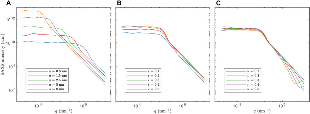
FIGURE 3. Examples of simulated SAXS curves. In (A), a is varied for ϵ =0.3 and ν =0 (two-phase model). In (B), ϵ is varied for a =2.5 nm and ν =0 (two-phase model). In (C), ν is varied for a =2.5 nm and ϵ =0.3 (three-phase model). For clarity, measurement noise has not been added to these curves.

2.4 Prediction of model parameters

The classical approach to estimating parameters in a model would be some variety of curve fitting, using e.g. least squares to find a scattering intensity curve that deviates minimally from the data and extract its parameters. However, predicting the model parameters can alternatively be considered a nonlinear regression and supervised learning problem: given a set of inputs i.e. the scattering intensities and the corresponding outputs i.e. the model parameters, find a function that approximates the mapping from input to output. Virtually any machine learning method for regression can be used in this setting. We rely on XGBoost (Chen and XGBoost, 2016), a specific implementation of gradient boosted trees. XGBoost has proven useful and accurate in another recent SAXS study where it was found to be superior to several other methods (Tomaszewski et al., 2021). Conveniently, and contrarily to some other candidate methods, XGBoost provides support for GPU acceleration. The orders-of-magnitude speedup delivered by the GPU acceleration makes XGBoost a particularly pragmatic choice for experiments involving large amounts of data, as it significantly shortens the experimentation time. The prediction model is a tree ensemble that combines a large number of weak, decision tree-based prediction models to produce a single, stronger prediction model. Each regression tree is constructed by recursively splitting the input data space into partitions or “branches”. After a sufficient amount of splitting, the space is divided into “leafs”, where each leaf corresponds to a single, scalar value which is the prediction of the output. Whereas a single regression tree is a poor approximation to the function mapping input to output, combining a large number of regression trees is a very powerful approach with performance on par with artificial neural networks. While deep neural networks dominate machine learning for computer vision and natural language processing, tree ensemble methods are generally the recommended approach for tabular data (Shwartz-Ziv and Armon, 2022).

The inputs of the training set are first preprocessed by transforming to logarithmic scale. Then, they are standardized by computing the mean and variance for each dimension separately on the training set, and then rescaling to zero mean and unit variance. Finally, the same rescaling (using the mean and variance of the training set) is applied to the validation and test sets (and also to new data once the prediction model is finalized and used). The outputs are not preprocessed. During training, the trees of the XGBoost model are optimized with respect to mean squared error (MSE) loss,

$\mathrm{M}\mathrm{S}\mathrm{E}=⟨{\left(\widehat{y}-y\right)}^2⟩,(13)$

where y is a target value and $\widehat{y}$ is a predicted value. Note that regression trees can inherently only be used to produce scalar predictions; hence, separate models are trained for each of the (scalar) outputs. The performance of XGBoost is affected by a number of hyperparameters. Refraining from going into too much detail, the parameters control the speed of learning, size and detail of the trees, random subsampling of both samples and input dimensions for each tree, regularization, and the number of trees. We list the ones that we explore further in Table 1, together with a concise explanation of their meaning and the ranges we investigate. The effect of the hyperparameters is investigated using a random search optimization, jointly for all hyperparameters (Bergstra and Bengio, 2012). The choice of which hyperparameters to study and their ranges are selected after an initial investigation. Because of the computational workload, this is performed only for the ϵ parameters (ϵ and ν are the hardest to predict, and of those only ϵ is present in all datasets). The results led to the following hyperparameters being used for all cases: learning_rate = 0.005, max_depth = 15, min_child_weight = 3, subsample = 0.15, colsample_bytree = 0.15, reg_lambda = 0.2, and max_bin = 1,024. Then, for all 10 outputs, training is performed with these values and n_estimators = 50,000. Further, for every output, 10 training runs are performed and the best-performing model is selected. We also use an early stopping rule that finalizes the training if no improvement is found for the last 1,000 added trees, and the best-performing model (best value of n_estimators) is selected. Therefore, in practice, the values of n_estimators in the final models vary from 6,060 to 48,841. Other than the hyperparameters stated, the default XGBoost settings are used. The training is run on NVIDIA A100 GPUs. The average execution time is approximately 3 h.

TABLE 1

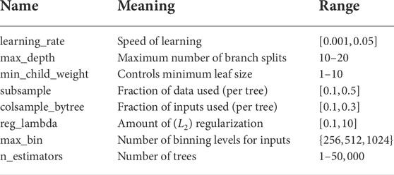
TABLE 1. List of hyperparameters investigated, with a brief explanation of their meaning and range of their values.

The results for the final selected XGBoost models is shown in Table 2. In addition to MSE, we also use the more intuitive mean absolute percentage error (MAPE) loss,

$\mathrm{M}\mathrm{A}\mathrm{P}\mathrm{E}=100\cdot ⟨\left|\frac{\widehat{y}-y}{y}\right|⟩\%.(14)$

TABLE 2

TABLE 2. Error measures for the prediction of the parameters, where MSE and MAPE (in %) is given for the training, validation and test sets.

Further, in Figures 4, 5, we show scatter plots of the predictions of all parameters for the test sets. We note that the scaling parameter a is consistently the easiest to predict in terms of MAPE (considering the substantial impact of the value of a on both the length and magnitude of the low-q plateau as seen in Figure 3, this is no surprise), but evidently a bit more difficult for increasing values of a because the relative error increases (not shown). This might be partly because of resolution limitations for low values of q (the simulated values of I(q) for low q is based on a very small number of grid points in q space; and large length scales i.e. large a correspond to low q). Also, the porosity ϵ is consistently the most difficult to predict. Finally, the fraction ν of the pore spaced filled up by intermediate layer is predicted a bit better than ϵ, but has more pronounced outliers in the low porosity case, in particular for low ν. This is likely because the fraction of the third phase is very low for low values of both ϵ and ν, and therefore the simulated SAXS data contains very limited information about that phase. For all parameters, the predictions have a positive bias near the lower bound of the range of true values. Likewise, the predictions have a negative bias near the upper bound of the range of true values. This is simply because the models are not trained to predict values outside the range and hence are unlikely to make such predictions. This fact also illustrates very clearly that the models cannot be expected to extrapolate well, but will rather provide reasonable predictions only within the domain of applicability (Sutton et al., 2020), which is determined by the distribution of inputs and outputs in the training set and the prediction model itself. It is also worth pointing out that if the prediction model would have been trained to predict the porosity on the low-porosity and the high-porosity data jointly, the predicted values would be nonsensical, and accordingly, the reported accuracy would be substantially lower.

FIGURE 4

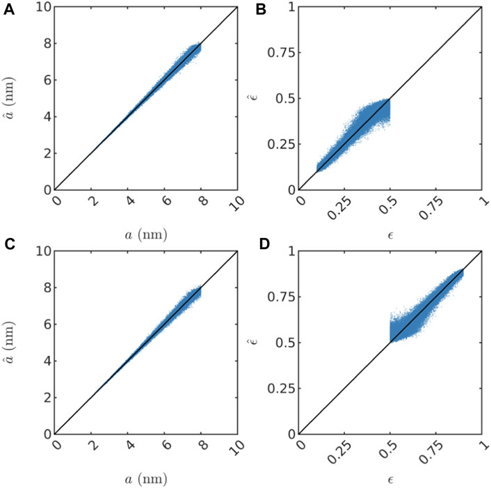
FIGURE 4. Scatter plots showing prediction results on the test set for both two-phase datasets. In (A,B), predictions of a and ϵ are shown for the two-phase low porosity structures. In (C,D), predictions of a and ϵ are shown for the two-phase high porosity structures.

FIGURE 5

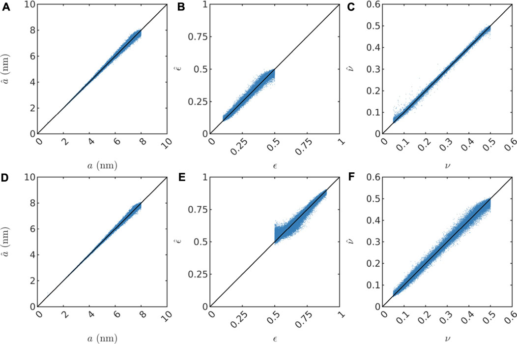
FIGURE 5. Scatter plots showing prediction results on the test set for both three-phase datasets. In (A–C), predictions of a, ϵ, and ν are shown for the three-phase low porosity structures. In (D–F), predictions of a, ϵ, and ν are shown for the three-phase high porosity structures.

In this context, it is important to note that the structures are random and not uniquely defined by the set of parameter values used to generate them; each set of parameter values can yield a very large number of different structures that in turn yield an equal number of different SAXS curves. Therefore, a SAXS curve cannot be uniquely mapped to a set of parameter values, even in the absence of measurement noise; their relationship is inherently random. It follows that the prediction loss is due to a combination of the randomness of the structures and the randomness induced by the added measurement noise. Therefore, there is in practice a lower bound on the attainable accuracy. This effect is essentially a result of the limited resolution and field of view of the simulated data and not as such a fundamental limitation of SAXS.

It is worth noting that we investigate two other techniques for regression. The first is also based on XGBoost but utilizing chained regression. This means that the different outputs are predicted sequentially such that the predictions of the first are used as input for prediction of the second, and the predictions of the first and second are used as inputs for prediction of the third. Also we investigate fully-connected artificial neural networks. An initial investigation suggests that neither of these two attempts yield better results than the ‘plain’ XGBoost approach presented, and are therefore not shown herein.

2.5 Simulated case study

To illustrate the performance of the method more clearly, we do a case study on simulated data using the three-phase model. Because the prediction model does not capture variability, the uncertainty of the predictions cannot be assessed using a single SAXS measurement. Therefore, we simulate a large number of measurements using the same parameter values, akin to performing replicate real measurements. Indeed, for a = 4 nm, ϵ = 0.70, and ν = 0.20, we generate 500 SAXS curves with the same noise model as before and use the three-phase high porosity model for prediction. The results are shown in Figure 6. The combined results are $\widehat{a}=4.004\pm 0.025$ nm, $\widehat{ϵ}=0.701\pm 0.009$, and $\widehat{\nu }=0.201\pm 0.005$ (m ± sd). In this case (for the three-phase high porosity model), the average execution time for prediction is 2.5 m for each SAXS curve and all three predicted outputs; however, this depends on the model complexity (i.e. the value of n_estimators). Note that this execution time only reflects the prediction as such and not loading and preprocessing of data and saving predictions. Further, the results for a single structure are shown in Figure 7, showing the simulated 1D SAXS curve from both the true structure and a reconstructed structure using the predicted parameter values (in this case $\widehat{a}=3.982$ nm, $\widehat{ϵ}=0.706$, and $\widehat{\nu }=0.195$) as well as representative slices from the true and reconstructed structures. In the high q range, the reconstructed SAXS curve reasonably well reproduces that of the true structure. In the low q range, there is a larger discrepancy. However, due to the simulated SAXS curves being an average of very few values of I(q) for low q, the random fluctuations between different structures will be larger in that range.

FIGURE 6

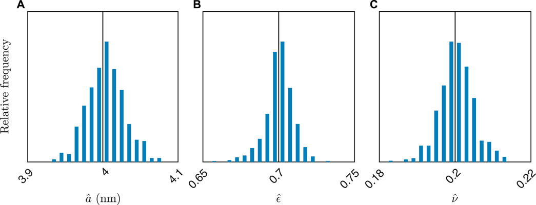
FIGURE 6. Histogram of estimated values for 500 simulated SAXS curves for a = 4 nm, ϵ = 0.70, and ν = 0.20. In (A–C), the distribution of estimated values of a, ϵ, and ν are shown. The true values are also indicated (vertical black lines).

FIGURE 7

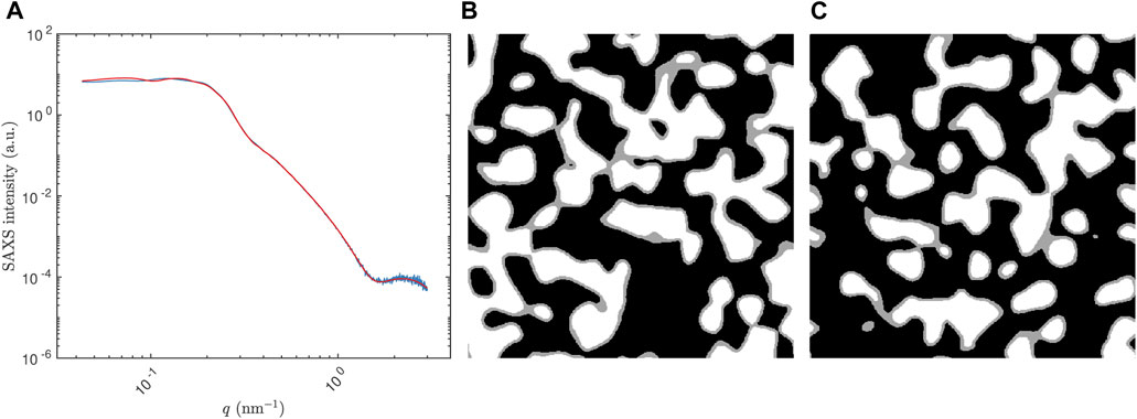
FIGURE 7. Results for a single structure in the case study. In (A), the simulated SAXS curve for a =4 nm, ϵ =0.70, and ν =0.20 (blue), and a (noiseless) SAXS curve of a structure generated using the predicted parameters $\widehat{a}=3.982$ nm, $\widehat{ϵ}=0.706$, and $\widehat{\nu }=0.195$ (red) are shown. In (B,C), single slices from the true structure and the reconstructed structure are shown, showing pore (black), water (gray), and solid (white).

3 Conclusion

We have implemented a machine learning-based approach to fast estimation of microstructural parameters from SAXS data. The microstructure model is based on a periodic Gaussian random field with variable length scale, which is processed and thresholded to yield two-phase (pore and solid) and three-phase (pore, intermediate layer, and solid) structures, with all phases having different electron densities. We also develop a Fourier transform-based method to simulate SAXS data. Both microstructure generation and SAXS simulation are implemented on the GPU and very fast. We generate four very large, separate datasets: 1) two-phase, low porosity structures 2) two-phase, high porosity structures, 3) three-phase, low porosity structures, and 4) three-phase, high porosity structures. We demonstrate that by performing regression using XGBoost, a decision tree-based machine learning framework, the parameters of the models can be predicted with good accuracy. Given that artificial neural networks did not perform better than XGBoost, and given that there is no time dependence or translational invariance in the data to further exploit, it is unlikely that more advanced architectures such as recurrent or convolutional neural networks would perform better. Further, the parameter prediction executes virtually instantaneously. Hence the computational burden of conventional model fitting can be avoided, enabling for the SAXS practitioner to efficiently analyze many measurements.

We observed positive and negative bias in the predictions observed near the lower and upper bound of the simulated parameter ranges. This bias could be reduced by using a wider range of parameters (where possible) for the training set while maintaining the ranges for the validation and test sets. In this manner, the performance of the prediction will be assessed in a smaller parameter space, which should then be considered the domain of applicability.

Although the microstructure models herein are aimed at mimicking a certain type of morphology and certain ranges of the parameters, similar models can be expected to perform well for other types of microstructures (i.e., fibers, foams, granules) and other parameter ranges. The only requirement is that the microstructure model is efficiently implemented so that a large, representative dataset can be generated, and that the corresponding SAXS curves are sufficiently informative regarding the parameters to be predicted. Although the approach is evaluated on a specific type of morphology, it is a proof of concept that can be used for other types of materials, both with regard to spatial structure and electron density values, and also for other experimental parameters such as other q value ranges, and non-equidistant q values. Indeed, generalizing this investigation to multiple classes of Gaussian random field-based models would be an interesting prospect for further work.

In conclusion, this proof of concept illustrates the usefulness not only of the machine learning-based approached but also of the efficient GPU-accelerated scheme for simulating the materials structures and the corresponding SAXS data and the new three-phase model. Finally, all the data and codes used herein are publicly available to facilitate further development in this field.

Data availability statement

The datasets presented in this study can be found in online repositories. The names of the repository/repositories and accession number(s) can be found below: DOI:10.5281/zenodo.5948941.

Author contributions

SY and JR conceived the idea. MR developed the microstructure generation and SAXS simulation methods together with SY. MR, PT, and MB developed the machine learning methods. MR and JR coordinated the work. All authors contributed to designing the study and to writing the manuscript.

Funding

MR acknowledges the financial support of the Swedish Research Council for Sustainable Development (grant number 2019-01295). SY acknowledges the financial support of the Swedish Research Council (grant number 2018-06378).

Acknowledgments

The computations were in part performed on resources at Chalmers Centre for Computational Science and Engineering (C3SE) provided by the Swedish National Infrastructure for Computing (SNIC).

Conflict of interest

The authors declare that the research was conducted in the absence of any commercial or financial relationships that could be construed as a potential conflict of interest.

Publisher’s note

All claims expressed in this article are solely those of the authors and do not necessarily represent those of their affiliated organizations, or those of the publisher, the editors and the reviewers. Any product that may be evaluated in this article, or claim that may be made by its manufacturer, is not guaranteed or endorsed by the publisher.

References

Archibald, R. K., Doucet, M., Johnston, T., Young, S. R., Yang, E., and Heller, W. T. (2020). Classifying and analyzing small-angle scattering data using weighted k nearest neighbors machine learning techniques. J. Appl. Crystallogr. 53, 326–334. doi:10.1107/s1600576720000552

CrossRef Full Text | Google Scholar

Barman, S., Rootzén, H., and Bolin, D. (2019). Prediction of diffusive transport through polymer films from characteristics of the pore geometry. AIChE J. 65, 446–457. doi:10.1002/aic.16391

CrossRef Full Text | Google Scholar

Bergstra, J., and Bengio, Y. (2012). Random search for hyper-parameter optimization. J. Mach. Learn. Res. 13, 281.

Google Scholar

Berk, N. F. (1991). Scattering properties of the leveled-wave model of random morphologies. Phys. Rev. A . Coll. Park. 44, 5069–5079. doi:10.1103/physreva.44.5069

PubMed Abstract | CrossRef Full Text | Google Scholar

Blanchet, C. E., and Svergun, D. I. (2013). Small-angle X-ray scattering on biological macromolecules and nanocomposites in solution. Annu. Rev. Phys. Chem. 64, 37–54. doi:10.1146/annurev-physchem-040412-110132

PubMed Abstract | CrossRef Full Text | Google Scholar

Cahn, J. W., and Hilliard, J. E. (1958). Free energy of a nonuniform system. I. Interfacial free energy. J. Chem. Phys. 28, 258–267. doi:10.1063/1.1744102

CrossRef Full Text | Google Scholar

Chen, S. H., Lee, D. D., Kimishima, K., Jinnai, H., and Hashimoto, T. (1996). Measurement of the Gaussian curvature of the surfactant film in an isometric bicontinuous one-phase microemulsion. Phys. Rev. E 54, 6526–6531. doi:10.1103/physreve.54.6526

PubMed Abstract | CrossRef Full Text | Google Scholar

Chen, T., and XGBoost, C. G. (2016). “A scalable tree boosting system,” in Proceedings of the 22nd ACM SIGKDD Conference on Knowledge Discovery and Data Mining, San Francisco, CA, USA, August 13-17, 2016, 785–794.

Google Scholar

Chu, B., and Hsiao, B. S. (2001). Small-angle X-ray scattering of polymers. Chem. Rev. 101, 1727–1762. doi:10.1021/cr9900376

PubMed Abstract | CrossRef Full Text | Google Scholar

D’hollander, S., Gommes, C. J., Mens, R., Adriaensens, P., Goderis, B., and Du Prez, F. (2010). Modeling the morphology and mechanical behavior of shape memory polyurethanes based on solid-state NMR and synchrotron SAXS/WAXD. J. Mat. Chem. 20, 3475–3486. doi:10.1039/b923734h

CrossRef Full Text | Google Scholar

Do, C., Chen, W.-R., and Lee, S. (2020). Small angle scattering data analysis assisted by machine learning methods. MRS Adv. 5, 1577–1584. doi:10.1557/adv.2020.130

CrossRef Full Text | Google Scholar

Feinauer, J., Brereton, T., Spettl, A., Weber, M., Manke, I., and Schmidt, V. (2015). Stochastic 3D modeling of the microstructure of lithium-ion battery anodes via Gaussian random fields on the sphere. Comput. Mater. Sci. 109, 137–146. doi:10.1016/j.commatsci.2015.06.025

CrossRef Full Text | Google Scholar

Franke, D., Jeffries, C. M., and Svergun, D. I. (2018). Machine learning methods for X-ray scattering data analysis from biomacromolecular solutions. Biophysical J. 114, 2485–2492. doi:10.1016/j.bpj.2018.04.018

CrossRef Full Text | Google Scholar

Geslin, P.-A., McCue, I., Gaskey, B., Erlebacher, J., and Karma, A. (2015). Topology-generating interfacial pattern formation during liquid metal dealloying. Nat. Commun. 6 (1–8), 8887. doi:10.1038/ncomms9887

PubMed Abstract | CrossRef Full Text | Google Scholar

Gommes, C. J., and Roberts, A. P. (2018). Stochastic analysis of capillary condensation in disordered mesopores. Phys. Chem. Chem. Phys. 20, 13646–13659. doi:10.1039/c8cp01628c

PubMed Abstract | CrossRef Full Text | Google Scholar

Gommes, C. J., and Roberts, A. P. (2008). Structure development of resorcinol-formaldehyde gels: Microphase separation or colloid aggregation. Phys. Rev. E 77, 041409. doi:10.1103/physreve.77.041409

PubMed Abstract | CrossRef Full Text | Google Scholar

Gommes, C. J. (2018). Stochastic models of disordered mesoporous materials for small-angle scattering analysis and more. Microporous Mesoporous Mater. 257, 62–78. doi:10.1016/j.micromeso.2017.08.009

CrossRef Full Text | Google Scholar

Gommes, C. J. (2013). Three-dimensional reconstruction of liquid phases in disordered mesopores using in situ small-angle scattering. J. Appl. Crystallogr. 46, 493–504. doi:10.1107/s0021889813003816

CrossRef Full Text | Google Scholar

He, H., Liu, C., and Liu, H. (2020). Model reconstruction from small-angle X-ray scattering data using deep learning methods. iScience 23, 100906. doi:10.1016/j.isci.2020.100906

PubMed Abstract | CrossRef Full Text | Google Scholar

Henke, B. L., Gullikson, E. M., and Davis, J. C. (1993). X-Ray interactions: Photoabsorption, scattering, transmission, and reflection at E = 50-30, 000 eV, Z = 1-92. Atomic Data Nucl. Data Tables 54, 181–342. doi:10.1006/adnd.1993.1013

CrossRef Full Text | Google Scholar

Jinnai, H., Hashimoto, T., Lee, D., and Chen, S.-H. (1997). Morphological characterization of bicontinuous phase-separated polymer blends and one-phase microemulsions. Macromolecules 30, 130–136. doi:10.1021/ma960486x

CrossRef Full Text | Google Scholar

Lang, A., and Potthoff, J. (2011). Fast simulation of Gaussian random fields. Monte Carlo Methods Appl. 17, 195–214. doi:10.1515/mcma.2011.009

CrossRef Full Text | Google Scholar

Li, T., Senesi, A. J., and Lee, B. B. (2016). Small angle X-ray scattering for nanoparticle research. Chem. Rev. 116, 11128–11180. doi:10.1021/acs.chemrev.5b00690

PubMed Abstract | CrossRef Full Text | Google Scholar

Liu, Y., Li, J., Sun, S., and Yu, B. (2019). Advances in Gaussian random field generation: A review. Comput. Geosci. 23, 1011–1047. doi:10.1007/s10596-019-09867-y

CrossRef Full Text | Google Scholar

Lu, Z., Li, C., Han, J., Zhang, F., Liu, P., Wang, H., et al. (2018). Three-dimensional bicontinuous nanoporous materials by vapor phase dealloying. Nat. Commun. 9 (1–7), 276. doi:10.1038/s41467-017-02167-y

PubMed Abstract | CrossRef Full Text | Google Scholar

Matérn, B. (1986). Spatial variation. New York: Springer.

Google Scholar

Nishi, Y. (2014). “2 - past, present and future of lithium-ion batteries: Can new technologies open up new horizons?,” in Lithium-ion batteries. Editor G. Pistoia (Amsterdam: Elsevier), 21–39.

CrossRef Full Text | Google Scholar

Prifling, B., Röding, M., Townsend, P., Neumann, M., and Schmidt, V. (2021). Large-scale statistical learning for mass transport prediction in porous materials using 90, 000 artificially generated microstructures. Front. Mat. 8, 786502. doi:10.3389/fmats.2021.786502

CrossRef Full Text | Google Scholar

Quintanilla, J. A., Chen, J. T., Reidy, R. F., and Allen, A. J. (2007). Versatility and robustness of Gaussian random fields for modelling random media. Model. Simul. Mat. Sci. Eng. 15, S337–S351. doi:10.1088/0965-0393/15/4/s02

CrossRef Full Text | Google Scholar

Roberts, A. P. (1997). Morphology and thermal conductivity of model organic aerogels. Phys. Rev. E 55, R1286–R1289. doi:10.1103/physreve.55.r1286

CrossRef Full Text | Google Scholar

Röding, M., Ma, Z., and Torquato, S. (2020). Predicting permeability via statistical learning on higher-order microstructural information. Sci. Rep. 10, 15239. doi:10.1038/s41598-020-72085-5

PubMed Abstract | CrossRef Full Text | Google Scholar

Scherdel, C., Miller, E., Reichenauer, G., and Schmitt, J. (2021). Advances in the development of sol-gel materials combining small-angle X-ray scattering (SAXS) and machine learning (ML). Processes 9, 672. doi:10.3390/pr9040672

CrossRef Full Text | Google Scholar

Schmidt-Rohr, K. (2007). Simulation of small-angle scattering curves by numerical Fourier transformation. J. Appl. Crystallogr. 40, 16–25. doi:10.1107/s002188980604550x

CrossRef Full Text | Google Scholar

Sedlak, S. M., Bruetzel, L. K., and Lipfert, J. (2017). Quantitative evaluation of statistical errors in small-angle X-ray scattering measurements. J. Appl. Crystallogr. 50, 621–630. doi:10.1107/s1600576717003077

PubMed Abstract | CrossRef Full Text | Google Scholar

Shwartz-Ziv, R., and Armon, A. (2022). Tabular data: Deep learning is not all you need. Inf. Fusion 81, 84–90. doi:10.1016/j.inffus.2021.11.011

CrossRef Full Text | Google Scholar

Sorbier, L., Moreaud, M., and Humbert, S. (2019). Small-angle X-ray scattering intensity of multiscale models of spheres. J. Appl. Crystallogr. 52, 1348–1357. doi:10.1107/s1600576719013839

CrossRef Full Text | Google Scholar

Sutton, C., Boley, M., Ghiringhelli, L. M., Rupp, M., Vreeken, J., and Scheffler, M. (2020). Identifying domains of applicability of machine learning models for materials science. Nat. Commun. 11 (1–9), 4428. doi:10.1038/s41467-020-17112-9

PubMed Abstract | CrossRef Full Text | Google Scholar

Taylor, G. (2003). The phase problem. Acta Crystallogr. D. Biol. Crystallogr. 59, 1881–1890. doi:10.1107/s0907444903017815

PubMed Abstract | CrossRef Full Text | Google Scholar

Teubner, M. (1991). Level surfaces of Gaussian random fields and microemulsions. Europhys. Lett. 14, 403–408. doi:10.1209/0295-5075/14/5/003

CrossRef Full Text | Google Scholar

Tomaszewski, P., Yu, S., Borg, M., and Rönnols, Jerk (2021). “Machine learning-assisted analysis of small angle X-ray scattering,” in Proceedings of the 2021 Swedish Workshop on Data Science, Växjö, Sweden, December 2-3, 2021.1–6

PubMed Abstract | CrossRef Full Text | Google Scholar

Torquato, S. (2010). Optimal design of heterogeneous materials. Annu. Rev. Mat. Res. 40, 101–129. doi:10.1146/annurev-matsci-070909-104517

CrossRef Full Text | Google Scholar

Welborn, S. S., and Detsi, E. (2020). Small-angle X-ray scattering of nanoporous materials. Nanoscale Horiz. 5 (12–24), 12–24. doi:10.1039/c9nh00347a

CrossRef Full Text | Google Scholar

Zhang, H., Scholz, A. K., Jordan de, C., Vion-Loisel, F., Besnard, G., Alexander, H., et al. (2012). Nanocavitation in carbon black filled styrene–butadiene rubber under tension detected by real time small angle X-ray scattering. Macromolecules 45, 1529–1543. doi:10.1021/ma2023606

CrossRef Full Text | Google Scholar