Gas-assisted electrospinning of high-performance ceramic fibers: Optimal design modelling and experimental results of the gas channel of the nozzle

1 Introduction

Traditional ceramic fiber materials are usually prepared from ceramic oxide particles, and the inherent brittleness of ceramic materials greatly limits their application (Dan et al., 2003; Xu et al., 2018; Jia et al., 2022). After more than a decade of development, various methods for preparation of flexible ceramic fibers are discussed, including electrospinning, solution blow spinning, centrifugal spinning, self-assembly, chemical vapor deposition, atomic layer deposition, and polymer conversion (Luo et al., 2012; Ichikawa, 2016; Xu et al., 2018; Li et al., 2019; Cai et al., 2020; Calisir and Kilic, 2020; Ramlow et al., 2021). Among these preparation technologies, electrospinning is one of the most commonly used method for fabrication of ceramic fibers (Luo et al., 2012; Malwal and Gopinath, 2016; Hamid et al., 2017).

The main advantage of electrospinning is that the structure and morphology of the ceramic fiber can be easily controlled by adjusting the composition of the precursor solution, or alternation of spinning parameter and calcination conditions. However, electrospinning of ceramic fiber has mostly remained in the research level, which can be basically because of hard processes and parameters controlling and the low rate of production. Solution blow spinning has emerged as an alternative technique to produce sub-micron/nano sized fibers and can relieve the user of the limitations posed by electrospinning. The yield of fiber production is about hundred times higher than that of electrospinning, making it suitable for industrialization (Magaz et al., 2018; Tandon et al., 2019).

In this paper, using the advantages of solution blow spinning technology for reference, we prepared nanofiber by using assisted gas during the electrospinning process. As the nozzle design and the attenuation force are of utmost importance in gas-assisted electrospinning, both numerical and experimental methods were used to investigate the fiber formation. The optimal nozzle design parameters for gas reverse flow problem are studied using the finite element method. There is no bead formation in the actual production, which indicates that the optimized gas-assisted electrospinning can successfully produce high-performance ceramic fibers.

2 Fiber structure model and motion equation

Models used to simulate fibers include the “multi-sphere” model, “node-chain” model, and “bead-elastic rod” model (Yamamoto and Matsuoka, 1993; Kong and Platfoot, 1997). For the multi-sphere model, due to the large length-to-diameter ratio of the fiber, the model requires too many balls, resulting in too much calculation, and the model is not suitable for the high-speed airflow field. For the nodal chain model, when calculating the airflow resistance acting on the fiber segment, the straight-line distance between the nodes is used to represent the true length of the fiber segment, which often leads to a situation that is extremely inconsistent with the actual situation. For example, when the fiber segment is folded in half, the nodes at both ends overlap, and the straight-line distance between the nodes is zero, so the calculated airflow resistance is zero. In fact, the length of the fiber segment is half of the straight length at this time, and the airflow resistance received is not equal to zero. In comparison, the bead-elastic rod model is a better fiber model. In this study, we need to establish a fiber physical model that shows the elastic elongation and bending deformation of the polymer solution in the air flow field and can be simple and feasible in the numerical calculation. So we apply another model that can better reflect the characteristics of fibers “sphere-spring” model as a fiber model. This model has been used to simulate macromolecules in polymer dynamic structure (Bird et al., 1987). In this model, the elasticity of the fiber is reflected by the elasticity of the spring, and the flexibility of the fiber is reflected by the bendability of the spring. The “sphere-spring” fiber model is shown in Figure 1.

FIGURE 1

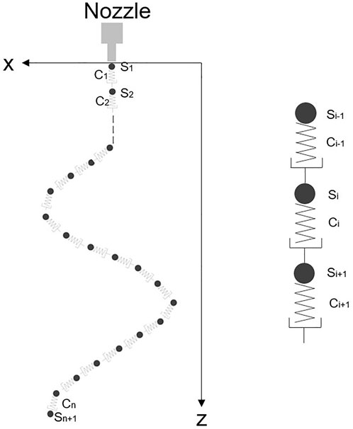
FIGURE 1. Fiber spinning model.

In Figure 1, S represents the sphere ball and C represents the connecting spring. The fiber is made up of n+1 balls connected by n massless springs. The mass $m_i$ of the $i$ ball is determined by the linear density of the fiber and the distance between two adjacent balls (fiber segment length). $m_i$ is

$m_i=\frac{{\rho }_f}{2}\left(l^{i-1}+l^i\right)(1)$

where ${\rho }_f$ is the linear density of the fiber, $l^{i-1}$ and $l^i$ are the lengths of the two springs connecting the ball $i,$ when $i=1$ or $i=n+1$, $l^0=l^{n+1}=0$.

The bending torque force $F_{ib}$ acting on the $i$ ball depends on the stiffness of the fiber and is expressed by formula (2), which has been explained in detail in the literature (Yamamoto and Matsuoka, 1993), and will not be repeated here.

$F_{ib}=-b\bullet ∆y_i(2)$

where $b$ is bending torque constant. The bending torque constant implies the rigidity of bending deformation, which is assumed to be a constant; $∆y_i$ is the deflection.

When the fiber in the particle phase moves in the flow field, it is mainly subjected to gravity, buoyancy, air resistance, additional mass force, pressure gradient force, Saffman lift, turbulent pulsating force, and thermophoretic force. Here, we only consider the main force of air resistance and ignore the influence of other forces. The resistance of the airflow acting on the fiber segment includes friction resistance and differential pressure resistance. The frictional resistance is caused by the speed difference between the airflow and the fiber, and the pressure differential resistance is related to the characteristic area of the fiber segment. For the $i$ connecting spring, these two forces can be calculated by the following two formulas.

$F_f^i=\frac{1}{2}{C}_f\rho A_t^i\left|u_t-v_{it}\right|\left(u_t-v_{it}\right)(\mathrm{3a})$

$F_p^i=\frac{1}{2}{C}_p\rho A_n^i\left|u_n-v_{in}\right|\left(u_n-v_{in}\right)(\mathrm{3b})$

where $F_f^i$ and $F_p^i$ represent frictional resistance and differential pressure resistance, respectively; where $C_f$ and $C_p$ are the frictional resistance coefficient and the differential pressure resistance coefficient, respectively. The specific calculation formula is shown in formula (4) (Ju and Shambaugh, 1994). $\rho$ is the density of air, $A_t^i$ and $A_n^i$ are the surface area and longitudinal cross-sectional area of the fiber section, respectively. $u_t$ and $v_{it}$ are the velocity of the air flow along the axial direction of the fiber section and the velocity of the ball, respectively; $u_n$ and $v_{in}$ are the velocity of the airflow along the normal direction of the fiber section and the velocity of the ball, respectively.

$C_f=0.78\times {\left(R_{e_l}\right)}^{-0.61}(\mathrm{4a})$

$C_p=6.96\times {\left(R_{e_d}\right)}^{-0.44}{\left(\frac{d}{d_0}\right)}^{0.404}(\mathrm{4b})$

In the aforementioned two formulas, $R_{e_l}$ and $R_{e_d}$ are the relative Reynolds number based on fiber straight length used when calculating surface friction resistance and differential pressure resistance, respectively; $d$ is the diameter of the fiber; $d_0$ is the reference diameter, equal to 78um.

The total resistance exerted on the fiber segment is

$F_d^i=F_f^i+F_p^i(5)$

The force on each ball is equal to half of the combined force of the resistance acting on the two springs connecting the ball, which is calculated by formula (6).

$\left.F_{id}=\frac{1}{2}{\left(F\right.}_d^{i-1}+F_d^i\right)(6)$

For the fiber model subjected to the aforementioned force, the following force balance equation can be used to describe the fiber movement.

$m_i\frac{d{v}_i}{dt}=F_{ib}+F_{id}+F_{i-1.i}+F_{i,i+1}(7)$

where $v_i$ is the speed of the $i$ ball; $F_{i-1.i}$ and $F_{i,i+1}$ are the forces between adjacent balls, which is the elastic restoring force of the spring.

Formula (7) is the governing equation of the fiber motion.

3 Simulation and analysis

3.1 Reverse flow phenomenon

During the spinning, whether it is electrospinning, gas-assisted electrospinning or solution blow spinning, there are gel problems on the spinning tip. The generation of gel is related to the concentration, temperature, and preservation time of the solution. In other words, the larger the concentration of the solution, the lower the temperature, and the longer the preservation time can promote the formation of gel.

In order to clarify the gel formation mechanism of different spinning technologies, Polyvinyl solution spinning experiments were performed with three different spinning technologies, as shown in Figure 2. As shown in Figures 2A–E, it was found that the gel appeared in front of the needle tip during the spinning without gas. In this experiment, the speed of the liquid supply was too large, resulting in the continuous output solution not being able to be stretched into fiber by the electric field. Due to the effect of gravity and electric field power, the position of the gel appears at the front and bottom of the spinning tip.

FIGURE 2

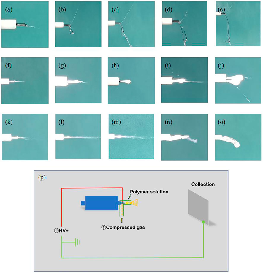
FIGURE 2. (A–E) is the spinning state of the 0, 1, 5, 10, and 15 min of ES; (F–J) is the spinning state of the 0, 1, 5, 10, and 15 min of GES; (K–O) is the spinning state of the 0, 1, 5, 10, 15, 15 min of SBS; (P) Schematic diagram of three spinning methods: while the polymer solution supply, (1) GES: turn on ①compressed gas and ②high-voltage power supply; (2) ES: turn off ①compressed gas and turn on ②high-voltage power supply; (3) SBS: turn on ①compressed gas and turn off ②high-voltage power supply.

As shown in Figures 2F–O, during the spinning with gas, the position of the gel appeared wrapped around the spinning needle. You could obviously see the phenomenon of interrupted spinning as shown in Figures 2H, N, O. This can be explained in the simulation model shown in Figure 3. The airflow of the needle under the streaming field conditions was simulated by the finite element analysis software shown in Figure 3. It can be seen from Figure 3B that at the front of the needle, there was obvious reverse flow phenomenon. This phenomenon had also been reported in the paper of the predecessors (Atif et al., 2020). Therefore, the gel appeared after the spinning process with gas was due to reverse flow at the front of the needle tip, and a certain disturbance was formed around the tip of the needle, which enhanced the volatilization of the solvent and increased the concentration of the solution near this needle tip. At the same time, the existence of a certain air pressure can reduce the local temperature due to the Joule–Thomson effect. So, the increase in concentration and decrease in temperature promoted gel formation. After a period of spinning, as the gel becomes larger, until the needle was completely blocked, the phenomenon of interrupted spinning would occur.

FIGURE 3

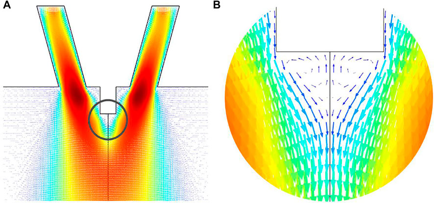
FIGURE 3. Speed vector diagram of the nozzle position: (A) Overall simulation map; (B) elimination of the needle tip.

By comparing Figures 2F–J and Figures 2K–O, it can be found that the needle tip was easier to completely block if spinning just by using gas flow. This is because if there is an auxiliary of electric field power, it could weaken the impact of reverse flow. The schematic diagram of the three spinning methods is shown in Figure 2P.

In summary, in the process of spinning with gas flow, reverse flow phenomenon is the biggest cause of the solution gel formation. Therefore, how to weaken the impact of reverse flow during spinning is of great research significance for the spinning technology.

In this paper, the max distance of the reverse flow, the max speed of the reverse flow, and the max speed of the positive flow are considered to be the relevant indicators of the strong or weak features of the reverse flow phenomenon. The shorter the max distance of the reverse flow is, the lower the max speed of the reverse flow becomes, and the higher the max speed of the positive flow is, the weaker the reverse flow phenomenon becomes.

3.2 Model optimization objective

3.2.1 Digital description of reverse flow in a simulation model

The airflow of the nozzle under the streaming field conditions was simulated by the finite element analysis software shown in Figure 3. There are high -pressure airflows on both sides of the needle, and the tip of the needle is a low -pressure area. Under the action of atmospheric pressure, some airflows will move closer to the tip of the needle, so as to form local reverse flow at the needle tip.

As shown in Figure 4, the gas-flow is sprayed from the +Z direction to the zero point. To create the coordinate system, the center point of the needle outlet is the center point, and the positive direction of the gas-flow speed is defined from zero to the +Z direction.

FIGURE 4

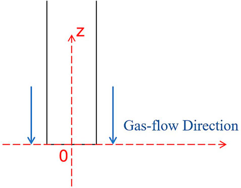
FIGURE 4. Coordinate system diagram of the gas-flow at the needle.

Draw a two-dimensional line of x = 0 in Figure 4, and calculate the speed of the gas-flow from 0 to Z in the direction of Z, which can get the relationship curve of the gas-flow speed in the direction of the Z direction as Figure 5 shown.

FIGURE 5

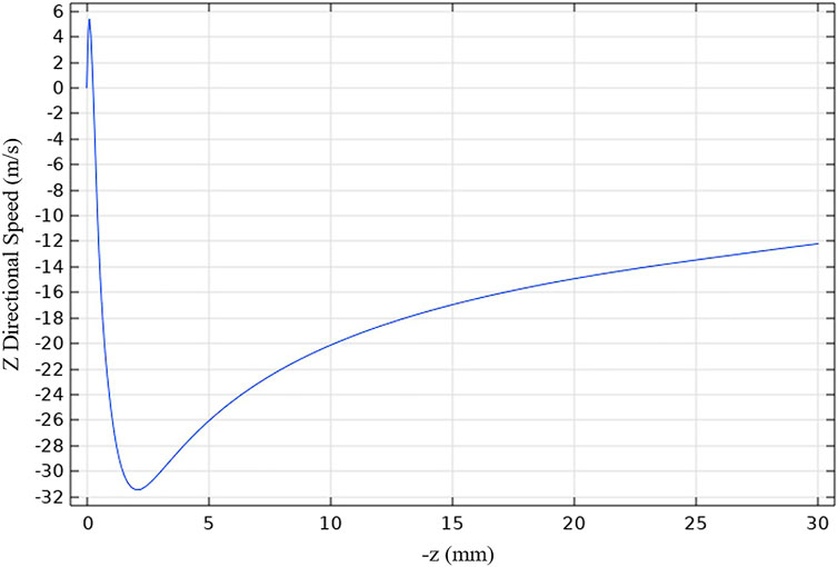
FIGURE 5. Curve of the gas-flow + Z direction speed at the -Z moving direction.

3.2.2 Objective and the method of optimization

In this paper, the max distance of the reverse flow, the max speed of the reverse flow, and the max speed of the positive flow would be used as the optimization objective of the reverse flow phenomenon problem. We would optimize the reverse flow phenomenon by changing the angles of nozzles, the needles size, and the length of needles tip exposed.

3.3 Effect of different flow angles on the max flow velocity, the max velocity, and distance of reverse flow

First, we established a two-dimensional axial symmetrical layer flow model in the finite element simulation software, and established a local solution domain of airflow speed changes for the nozzle position, which is conducive to reducing unnecessary calculation quantities to improve solution efficiency. Then the material of the solution domain was defined as the air domain, and defined the entrance and exit positions of the airflow were defined, as shown in the blue line label in Figure 6.

FIGURE 6

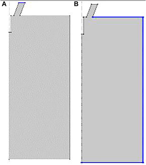
FIGURE 6. Boundary condition settings of the airflow import and export: (A) Blue line is entrance; (B) blue line is exit.

We set the airflow entry speed to 20 m/s, and the exit static pressure is set to 0Pa. In order to improve the convergence of the calculation results, we added the order jump function, and set the non-self-negative stability parameter δid of the layer flow module to 0.5, and then divided the grid of the model. The angle value was based on the surface of the needle exit, and the gas flow emitting direction was set to 30°, 45°, 60°, 75°, 90°, and 90°*, respectively. Among them, "*" means that before the gas flow leaves the nozzle, the airflow has been in contact with the inner needle. Adjusting the distance from the flow of the needle tip to 1mm, we set the flow field simulation in different angles of gas flowing. The simulation results are shown in Figure 7. The curve diagram drawn by the simulation calculation results of each angle is shown in Figure 8.

FIGURE 7

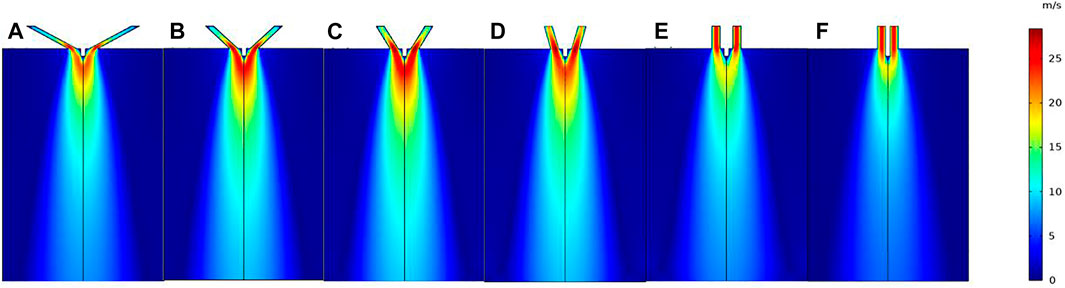
FIGURE 7. Flow speed distribution cloud map of different nozzles angle: (A) 30°; (B) 45°; (C) 60°; (D) 75°; (E) 90°; (F) 90°*.

FIGURE 8

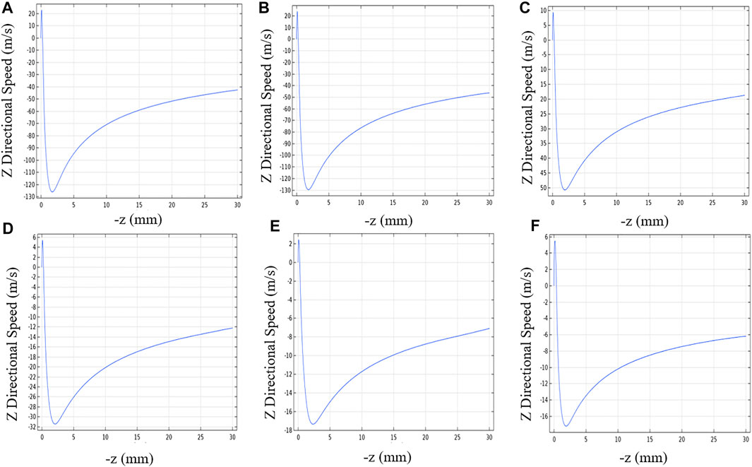
FIGURE 8. Curve of the gas-flow speed at the -Z direction at different angles: (A) 30°; (B) 45°; (C) 60°; (D) 75°; (E) 90°; (F) 90°*.

After sorting the aforementioned data, we draw the max flow velocity and the max distance of reverse flow diagram at different angles, shown in Figure 9. From Figure 9, when the angle is 90°*, the distance of reverse flow is the longest, and the max reverse flow speed is the minimum, so it can be seen that the angle is the best parameter of nozzle to solve the problem of reverse flow phenomenon.

FIGURE 9

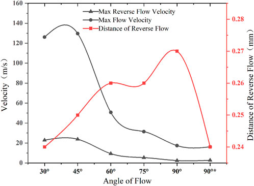
FIGURE 9. Folding diagram of the flow velocity and the distance of reverse flow at different angles.

3.4 Effect of the different needle size on the max flow velocity, the max velocity, and distance of reverse flow

From the results from Figure 9 and the simulation results of different length of needle tip, including 2, 3, and 4mm, it can be concluded that the distance of reverse flow is the longest, and the max reverse flow speed is the minimum when the angle is 90°*. Therefore, with an angle of 90°*, the exposure length of the needle was set to 8 mm, the inner diameter of the gas channel was set to 1.8 mm, and the gas flow was set to 15 L/min. We used the three different specifications of 20G (outer diameter 0.9 mm and inner diameter 0.6 mm), 23G (outer diameter 0.63 mm and inner diameter 0.33 mm), and 25G (outer diameter 0.51 mm and inner diameter 0.26 mm) to simulate and analysis, as shown in Figure 10.

FIGURE 10

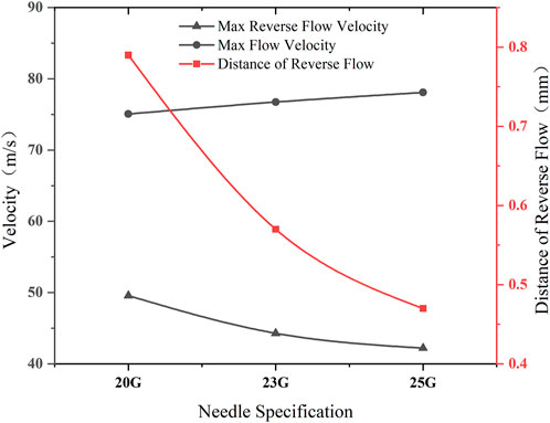
FIGURE 10. Folding diagram of the flow velocity and the distance of reverse flow at different needle specification.

It can be seen from Figure 10 that the max speed and the distance of the reverse flow is reduced as the diameter of the needle decreased, and the max speed of the positive current is also increased with the reduction of the diameter of the needle. Therefore, it is believed that the use of 25 G needles for spinning can solve the problem of reverse flow to the greatest extent.

3.5 Effect of different length of needle tip exposed on the max flow velocity, the max velocity, and distance of reverse flow

According to the simulation results of the previous chapter, for the structure of 90°*and 25 G needle, the length of needles tip exposed were set to 2 mm, 4 mm, 6 mm, and 8 mm. The folding diagram of the flow velocity and the distance of reverse flow at different length of tip exposed is shown in Figure 11.

FIGURE 11

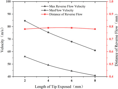
FIGURE 11. Folding diagram of the flow velocity and the distance of reverse flow at different length of tip exposed.

From the data of Figure 11, as the exposure length of the needle was increased, the maximum speed of the inverse flow was decreased but the change in the distance of reverse flow is not obvious, so the structure has a certain effect on reducing the phenomenon of reverse flow. Based on the consideration of optimization of reverse flow problems, this paper uses the exposure length of the needle tip of8 mm as the optimal parameter of the experimental data of the group.

4 Experiment and results

4.1 Study of air pressure for different needle tip

As shown in Figure 12, we set up an air pressure test device for different nozzles. Before accessing different nozzles, it was necessary to ensure that the compressor was filled with gases and it was stable. By adjusting the pressure regulating valve, the pressure indicator was displayed as 10.0 kPa, and immediately, the nozzle was accessed to read the air pressure data.

FIGURE 12

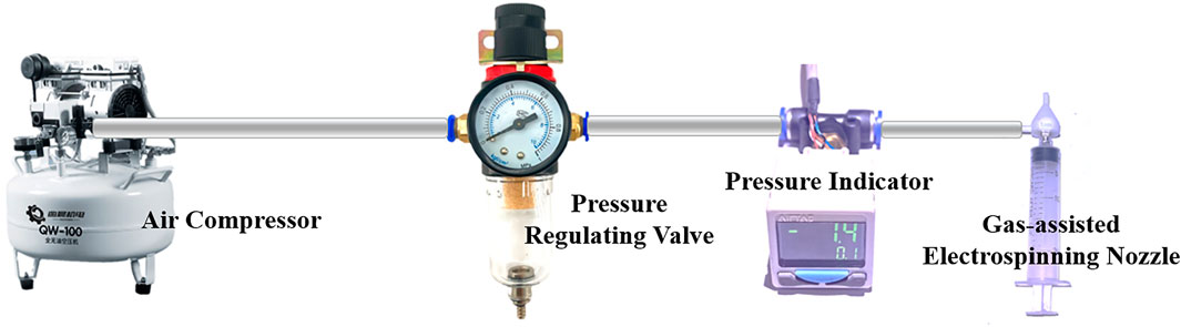
FIGURE 12. Schematic diagram of air pressure test device.

From the simulation and measured data comparison of Figure 13, it can be found that the larger the simulation speed, the smaller the measured air pressure value. This can be explained by Bernoulli’s theorem: the smaller the air pressure, the larger the airflow speed. It shows that the simulation results have certain reference significance to real situation.

FIGURE 13

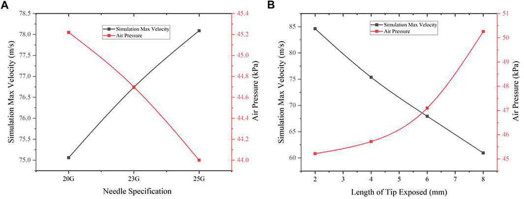
FIGURE 13. Comparison chart of the simulation data and measured data: (A) Different needle specifications; (B) Different needle tip exposed distance.

4.2 Preparation of high-performance ceramic fibers

4.2.1 Manufacturing process

4.2.1.1 Preparation of TEOS/PVA solution

Tetraethyl orthosilicate (TEOS, Aladdin), ionic water, and phosphate (Aladdin) were added into TEOS solution in the weight ratio of 1:2:0.005, respectively. Also, a 15wt% solution of polyvinyl alcohol (PVA220, Kuraray) in ion water was prepared. Finally, the TEOS solution was mixed with a PVA solution at a 1: 1 ratio to obtain the spinning solution.

4.2.1.2 Preparation of ultra-fine fiber membrane

According to the simulation and experimental results of the previous chapter, we chose an airflow nozzle with a 90°*, 8 mm length, and 23 G needle size because it will affect the supply of the solution if the diameter of the needle is too small. The TEOS/PVA solution was drawn into a 10-ml plastic syringe with a 23 G stainless steel needle. The needle was charged to 20 kV using a power supply and the mixture was pumped at a rate of 3 ml/h to the tip of the needle using a syringe pump. The auxiliary gas flow pressure controlled by the pressure regulating valve was set to 0.03 MPa. The needle was positioned 25 cm above a grounded collector with a 800rpm rate. A jet of the polymer solution was launched from the needle tip and was collected on the grounded surface, and ultra -fine fiber membrane was collected on the collector.

4.2.1.3 Preparation of ceramic fiber membrane

We placed the ultra-fine fiber membrane in the muffle furnace (Zhengzhou Xinhan Instrument Equipment Co., Ltd.), and the polymer composite fibers were in an air atmosphere and heated at a rate of 5°C/min until reaching 800°C. After maintaining the temperature for 3 h, the method of natural cooling was used to cool from high temperature to room temperature.

4.2.2 Characterization

The surface morphology of the nanofibers was observed by scanning electron microscopy (SEM, TESCAN MIRA3). The distribution of nanofiber diameters was calculated from the SEM images using ImageJ software (NIH, USA). We randomly selected 50 nanofibers from the SEM image to measure diameter, and finally made a diameter distribution diagram as shown in Figures 14C, D. The morphology of the PVA/SiO2 fibers was observed by SEM as shown in Figure 14A, with an average diameter of 310 nm. The nanofiber after burn is shown in Figure 14B, with an average diameter of 452nm, which is higher before the burning, indicating that nanofibers have a certain percentage of contraction in the direction of length, which can also prove it from the change in the area before and after the burning membrane.

FIGURE 14

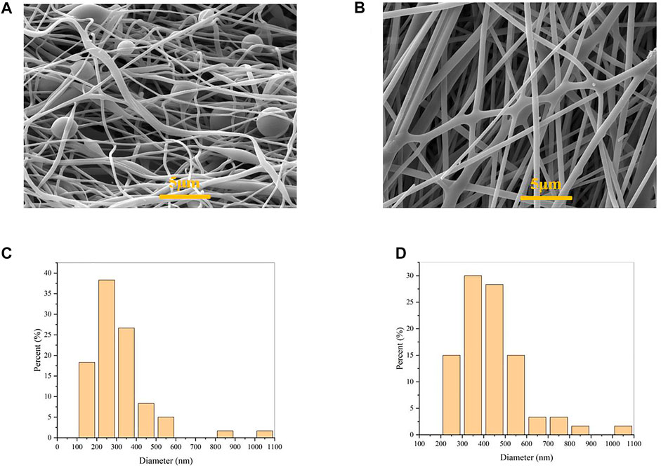
FIGURE 14. (A) SEM image of PVA/SiO2 nanofibers; (B) SEM image of ceramic nanofibers; (C) nanofiber diameter distribution graph of PVA/SiO2 nanofibers; (D) nanofiber diameter distribution graph of ceramic nanofibers.

The phase identification and crystallinity was obtained by using a wide angle X-ray diffraction (XRD, D8 Advance ECO) in the reflection mode with Cu-Ka radiation over Bragg 2h-angle ranging from 10–60. From Figure 15A, the strong and broad amorphous halo at 2θ = 22° in curve of three samples. It is the typical SiO2 widely drain peak, which also proves that the material is a non-fixed structure.

FIGURE 15

FIGURE 15. (A) XRD for SiO2 ceramic nanofibers; (B) flame retardant test; (C) heat insulation test.

The laser thermal conductor (LFA457, Netzsch) was used to test the thermal conductivity of SiO₂ nanofiber membrane, and the thermal diffusion coefficient was measured as 0.234 mm²/s under the condition of 230 V laser voltage and 25°C. In addition, Figures 15B, C also shows the actual flame retardant and thermal insulation effect of the SiO₂ fiber membrane.

5 Conclusion

The current research provides a comprehensive numerical and experimental analysis for nanofibers produced using gas-assisted electrospinning. The gas flow characteristics through different parameters' nozzle were investigated numerically using computational fluid dynamics and experimentally in a custom-built gas-assisted electrospinning setup to produce SiO₂ nanofibers.

In this paper, based on the consideration of optimization of reverse flow problems, it is believed that with 90°* as the nozzle angle, with 23 G as the needle specification, with 8 mm as the length of needle tip exposed is a set of best nozzle parameters. Taking these parameters as experimental conditions, the ceramic fibers prepared were tested or measured by SEM, XRD, and laser thermal conductor, which have proved that gas-assisted electrospinning can prepare high-performance ceramic fiber membranes. The results presented in the paper will pave the way for future research in fiber manufacturing using gas-assisted electrospinning.

Data availability statement

The original contributions presented in the study are included in the article/Supplementary Material; further inquiries can be directed to the corresponding authors.

Author contributions

All authors listed have made a substantial, direct, and intellectual contribution to the work and approved it for publication. Among the authors, GX, MC, and YG are equal, and are the joint first authors.

Funding

The authors gratefully acknowledge support from the Key-Area Research and Development Program of Guangdong Province (Grant No. 2019B010941001), 2019 Dong guan Postgraduate Joint Training (Practice) Workstation Project (Grant No. 2019707126017), Guangdong Basic and Applied Basic Research Foundation (Grant No. 2019A1515110432), Foshan Science and Technology Innovation Project (Grant No. 2020001004407).

Conflict of interest

Authors GX and JZ are employed by Foshan Nanofiberlabs Co., Ltd., China.

The remaining authors declare that the research was conducted in the absence of any commercial or financial relationships that could be construed as a potential conflict of interest.

Publisher’s note

All claims expressed in this article are solely those of the authors and do not necessarily represent those of their affiliated organizations, or those of the publisher, the editors, and the reviewers. Any product that may be evaluated in this article, or claim that may be made by its manufacturer, is not guaranteed or endorsed by the publisher.

References

Atif, R., Combrinck, M., Khaliq, J., Hassanin, A. H., Shyha, I., Elnabawy, E., et al. (2020). Solution blow spinning of high-performance submicron polyvinylidene fluoride fibres: Computational fluid mechanics modelling and experimental results. Polymers-Basel 12 (1140), 1140. doi:10.3390/polym12051140

PubMed Abstract | CrossRef Full Text | Google Scholar

Bird, R. B., Curtiss, C. F., Armstrong, R. C., and Hassager, O. (1987). Dynamics of polymeric liquids, volume 2, kinetic theory, 2nd edition. New York, United States: Wiley.

Google Scholar

Cai, Z., Su, L., Wang, H., Niu, M., Li, M., Gao, H., et al. (2020). Hydrophobic sic@C nanowire foam with broad-band and mechanically controlled electromagnetic wave absorption. Acs Appl. Mater Inter 12 (7), 8555–8562. doi:10.1021/acsami.9b20636

CrossRef Full Text | Google Scholar

Calisir, M., and Kilic, A. (2020). A comparative study on SiO2 nanofiber production via two novel non-electrospinning methods: Centrifugal spinning vs solution blowing. Mater Lett. 258 (1), 12675110. doi:10.1016/j.matlet.2019.126751

CrossRef Full Text | Google Scholar

Dan, L., Wang, Y., and Xia, Y. (2003). Electrospinning of polymeric and ceramic nanofibers as uniaxially aligned arrays. Nano Lett. 3 (8), 1167–1171. doi:10.1021/nl0344256

CrossRef Full Text | Google Scholar

Hamid, E., Rajan, J., and Seeram, R. (2017). Electrospun ceramic nanofiber mats today: Synthesis, properties, and applications. Materials 10 (11), 1238. doi:10.3390/ma10111238

PubMed Abstract | CrossRef Full Text | Google Scholar

Ichikawa, H. (2016). Polymer-derived ceramic fibers. Annu. Rev. Mater Res. 46, 335–356. doi:10.1146/annurev-matsci-070115-032127

CrossRef Full Text | Google Scholar

Jia, C., Xu, Z., Luo, D., Xiang, H., and Zhu, M. (2022). Flexible ceramic fibers: Recent development in preparation and application. Adv. Fiber Mater 4 (4), 573–603. doi:10.1007/s42765-022-00133-y

PubMed Abstract | CrossRef Full Text | Google Scholar

Ju, Y. D., and Shambaugh, R. L. (1994). Air drag on fine filaments at oblique and normal angles to the air stream. Polym. Eng. Sci. 34 (12), 958–964. doi:10.1002/pen.760341203

CrossRef Full Text | Google Scholar

Kong, L. X., and Platfoot, R. A. (1997). Computational two-phase air/fiber flow within transfer channels of rotor spinning machines. Text. Res. J. 67 (4), 269–278. doi:10.1177/004051759706700406

CrossRef Full Text | Google Scholar

Li, G., Zhu, M., Gong, W., Du, R., Eychmüller, A., Li, T., et al. (2019). Boron nitride aerogels with super-flexibility ranging from liquid nitrogen temperature to 1000 °C. Adv. Funct. Mater 29, 1900188. doi:10.1002/adfm.201900188

CrossRef Full Text | Google Scholar

Luo, C. J., Stoyanov, S. D., Stride, E., Pelan, E., and Edirisinghe, M. (2012). Electrospinning versus fibre production methods: From specifics to technological convergence. Chem. Soc. Rev. 41 (13), 4708–4735. doi:10.1039/c2cs35083a

PubMed Abstract | CrossRef Full Text | Google Scholar

Magaz, A., Roberts, A. D., Faraji, S., Nascimento, T., Medeiros, E. S., Zhang, W., et al. (2018). Porous, aligned and biomimetic fibers of regenerated silk fibroin produced by solution blow spinning. Biomacromolecules 19, 4542–4553. doi:10.1021/acs.biomac.8b01233

PubMed Abstract | CrossRef Full Text | Google Scholar

Malwal, D., and Gopinath, P. (2016). Fabrication and applications of ceramic nanofibers in water remediation: A review. Crit. Rev. Environ. Sci. Technol. 46 (5), 500–534. doi:10.1080/10643389.2015.1109913

CrossRef Full Text | Google Scholar

Ramlow, H., Marangoni, C., Motz, G., and Machado, R. A. F. (2021). Statistical optimization of polysilazane-derived ceramic: Electrospinning with and without organic polymer as a spinning aid for manufacturing thinner fibers - sciencedirect. Chem. Eng. J. Adv. 9, 100220. doi:10.1016/j.ceja.2021.100220

CrossRef Full Text | Google Scholar

Tandon, B., Kamble, P., Olsson, R. T., Blaker, J. J., and Cartmell, S. H. (2019). Fabrication and characterisation of stimuli responsive piezoelectric pvdf and hydroxyapatite-filled pvdf fibrous membranes. Molecules 24 (10), 1903. doi:10.3390/molecules24101903

PubMed Abstract | CrossRef Full Text | Google Scholar

Xu, C., Wang, H., Song, J., Bai, X., Liu, Z., Fang, M., et al. (2018). Ultralight and resilient Al2o3 nanotube aerogels with low thermal conductivity. J. Am. Ceram. Soc. 101, 1677–1683. doi:10.1111/jace.15301

CrossRef Full Text | Google Scholar

Yamamoto, S., and Matsuoka, T. (1993). A method for dynamic simulation of rigid and flexible fibers in a flow field. J. Chem. Phys. 98 (1), 644–650. doi:10.1063/1.464607

CrossRef Full Text | Google Scholar