Multiphysics simulation of an anisothermal reactive spontaneous capillary rise between electric rotor wires

1 Introduction

The rotor is the rotating component of an electric motor, while the stator is the static component, mainly consisting of copper wire coils. Two predominant technologies are used in the design of the rotor in electric vehicles: either a permanent magnet rotor or a copper wire wound rotor. The first currently offers better compacity and efficiency at maximum charge. However, the second, studied in this paper, provides the best efficiency across the wide range of speeds at which the vehicle is used thanks to its current modulation, which is crucial to make optimal use of the battery energy. Regarding the materials used, the wound style of rotor is also less critical in terms of both supply and recycling (Moragues et al., 2021). The wound rotor is composed primarily of a laminated steel core around which insulated copper wires are wound. Following this winding, the rotor is immersed in a liquid acrylate-based thermosetting resin bath.

Several publications in the literature deal with impregnated electrical coils: thermal parameters have been investigated (Simpson et al., 2013), and the aging of the insulation materials and experimental and simulation results in terms of their impact on electrical performance have been studied for rotor and stator cases (Loubeau, 2016; Nategh et al., 2014; Nategh et al., 2015). Studies on final product performance and material choices are also available; however, the manufacturing step is much less thoroughly documented, especially for wound rotors. Studies related to the impregnation step, in particular, were not identified for electric windings, unlike other fiber-impregnation applications for structural composite applications, such as carbon or glass fiber components. For electrical rotors, the role of good impregnation with resin is central for the application in order to:

• bind the wires (enabling them to resist vibrational, electromagnetic, and centrifugal forces: rotation speed rises to 12,000 rpm),

• improve insulation,

• resist chemical attacks and moisture, and

• improve thermal conductivity.

Resin impregnation between the wires occurs under controlled temperature settings to facilitate resin flow and polymerization. Unlike many composite processes, this does not involve pressurization to facilitate resin flow between the wires (of ≃ 1 mm in diameter). This suggests that capillary and gravity forces play a significant role in impregnation. The objective of the present study was to evaluate the impregnation quality of the windings under this type of processing conditions. Doing so requires characterization and simulation of a multi-material and multiphysics process in which phenomena such as heat transfer, polymerization kinetics, and resin flow are strongly coupled.

Before addressing the full-scale and fully coupled case, an intermediary step was implemented to understand the phenomena involved and validate the observations at a small scale (roughly half the rotor coil size in all directions). As presented in Moisy et al. (2022), an impregnation set-up (Figures 1A, B) was designed and optimized (including use a representative sample, design of an adapted impregnation follow-up method, and definition of a repeatable protocol). A heated aluminum mold containing a cavity was designed. The sample, referred to as a copper bar, consisted of 23 insulated copper wires aligned and positioned in the cavity (Figures 1C, D). The wires were 10 cm in length and ≃ 1 mm in diameter, and were organized in a compact hexagonal arrangement. The size of the resulting channels between the wires was ≃ 0.1 mm.

FIGURE 1

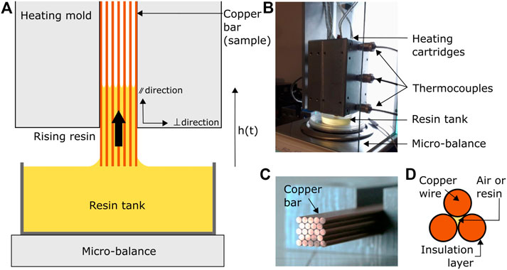
FIGURE 1. (A) Experimental set-up scheme and principles. (B) Experimental set-up. (C) View of the copper bar made up of 23 wires. (D) Schematic illustration of the composition, arrangement, and capillary cavity of three wires (Moisy et al., 2022).

Once the mold was closed, the sample was progressively brought closer to the resin surface; movement was stopped as soon as contact was created. The mold plus sample weight being high compared to the sensitivity needed to measure the resin intake, the strategy adopted to quantify capillary rise was to measure the loss of weight from the resin bath during the test. The aim was to perform these tests at controlled temperatures (room, 60, and 120°C). To achieve good homogenization of the temperature inside the copper bar, four long heaters were positioned in the aluminum mold. A sensor was placed between the heaters and the copper bar at mid-height to achieve smooth regulation. Weight evolution was recorded and post-treated using Matlab code to convert mass removed from the resin tank to a representation of height of capillary rise.

An associated model, neglecting inertia and polymerization, was optimized on the experimental capillary rise data (Figure 2).

FIGURE 2

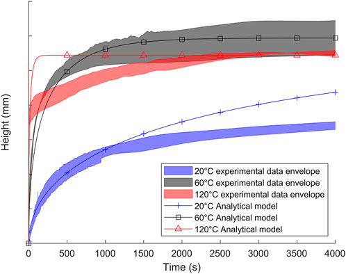
FIGURE 2. Comparison of experimental data and analytical model output (Fries and Dreyer, 2008) for impregnation via capillary rise (Moisy et al., 2022).

For temperatures of 20°C and 60°C, the capillary rise model (Fries and Dreyer, 2008) was found to describe the experimental results well up to 2,000 s (the period of interest for industrial applications). After 2,000 s, the equilibrium height remained a good fit for the 60°C and 120°C cases. The model was adjusted to provide a better fit at high temperatures than at the ambient temperature in order to match the process conditions more closely.

However, the model did not follow the peculiar experimental behavior in the 120°C case between 30 s and 2,000 s. The properties of some of the materials, particularly viscosity, may be undergoing evolution at 120°C. Polymerization advancement was not taken into account in this analytical model, and this may influence viscosity. In order to include this variable, a multiphysics simulation must be implemented. Similar coupled simulations can be found in the literature, including some of the physics of interest in this paper. For example, Nakouzi et al. (2010) present a simulation of the coupling between infrared heating and a polymerization reaction during liquid resin infusion; Keller et al. (2016) and Ou et al. (2017) provide simulations of heat transfer, polymerization kinetics, and fluid flow in a compression resin transfer molding process (epoxy resin and carbon fibers) and in thermoplastic elastomer injection, respectively.

Two main objectives were established for this study:

• to define a suitable model of impregnation able to reproduce via simulation the change of regime observed experimentally at 120°C, as well as describing the behavior at lower temperatures, and

• to understand the reasons and mechanisms underlying this change of regime by identifying the interactions between the predominant phenomena according to time and location in the sample.

2 Methods: Modeling choices and physics equations

2.1 Choice of scale and domain

Regarding the scale of the model, three options were available for investigation of the impregnation process:

• A single capillary (Chevalier et al., 2018) this option is relevant to develop a full understanding of the flow inside a single capillary cavity, but does not allow the full domain and the influence of its size and real boundary conditions to be taken into account.

• The cavities between many wires (Silva et al., 2016) full modeling would provide the most exhaustive description of the relevant phenomena. However, a fully coupled 3D simulation would be required and would be computationally expensive to perform for such a long processing period.

• A 2D homogenized domain [Keller et al. (2016); Ou et al. (2017)] local precision is lower, but the global phenomena and real boundary conditions can be reproduced at the duration of the experimental tests. This option is less computationally expensive than the preceding one.

The third alternative was selected for this model. The domain can further be described as a homogenized porous domain, which will be either dry or impregnated, with a macroscopic flow front follow-up.

The COMSOL Multiphysics software package, version 6.0, was used for modeling, along with the Computational Fluid Dynamics package.

To reflect the 3D geometry of the sample as far as possible in a 2D domain, an axisymmetric system was adopted. This enabled almost the entire sample to be captured (Figure 3) in a cylindrical shape of finite dimensions (Figure 4). The geometry of the porous network is not described. Instead, it is replaced with a homogenized anisotropic porous material, represented in grey (right of Figure 4). The sketch on the right-hand side of Figure 4 illustrates the geometry of the 2D homogeneous domain simulated; this choice was made in order to effectively simulate the entire sample within a reasonable calculation time.

FIGURE 3

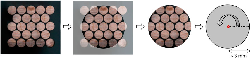
FIGURE 3. Perpendicular cross-section of the copper bar and representation as a homogenized porous medium of circular section.

FIGURE 4

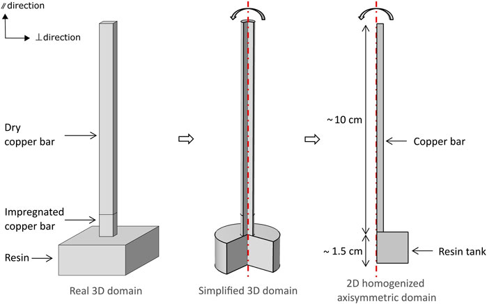
FIGURE 4. From the real 3D domain to the 2D axisymmetric domain.

2.2 Physics equations

The phenomena studied involved thermal exchanges, including exothermy of a polymerization reaction, and capillary-driven fluid flow of resin between wires. The relevant governing and constitutive equations for this work are presented accordingly in this section.

2.2.1 Thermal governing and constitutive equations

Assuming for the purpose of heat transfer analysis that a fibrous medium impregnated with resin forms a macroscopically homogeneous material, the conservation of energy is written (Advani and Sozer, 2010):

$\underset{\text{transient}}{\underbrace{\rho c\frac{\partial T}{\partial t}}}+\underset{\text{advection}}{\underbrace{\rho c\mathit{v}\cdot \mathrm{\nabla }T}}=\underset{\text{conduction\hspace{0.17em}}}{\underbrace{-\mathrm{\nabla }.\mathbf{q}}}+\underset{\text{viscous\hspace{0.17em}dissipation\hspace{0.17em}}}{\underbrace{\mathit{\tau }:\mathrm{\nabla }\mathit{v}}}+\underset{\text{energy\hspace{0.17em}generation\hspace{0.17em}}}{\underbrace{\dot{Q}}}(1)$

with T representing the spatial average temperature, v the phase average resin velocity, ρ the homogenized density, c the homogenized specific heat, q the heat flux vector, τ the viscous stress tensor, and $\dot{Q}$ the bulk energy generation. When low stresses are applied on the resin during the process, the viscous dissipation term of Eq. 1 is negligible.

Heat flux for the conduction phenomena can be regarded as proportional to the temperature gradient, as expressed by Fourier’s law:

$\mathbf{q}=-\mathit{\lambda }\mathrm{\nabla }T(2)$

where λ is the tensor of thermal conductivity coefficients.

For the thermosetting resin, the energy generation term is assimilated to the polymerization heat generation:

$\dot{Q}=-{\rho }_{\mathit{resin}}\mathrm{\Delta }{H}_r\frac{d\alpha }{dt}(3)$

with ΔH_r representing the total enthalpy of the reaction (J.kg^-1) (negative), determined during the DSC (Differential Scanning Calorimetry) study, and ρ_resin representing the resin density.

2.2.2 Flow governing equations and capillary pressure

As the domain was homogenized, the flow is not described microscopically in each channel, but is rather described globally, with a macroscopic front follow-up. The associated flow equations are presented in this section.

When the following assumptions are valid:

• the porosity ϵ of the fiber network is constant (fixed fibers),

• the resin flow is laminar,

• the resin density ρ_resin is constant (incompressible fluid),

• the porous medium is not multiscaled, so no local difference in kinetics of impregnation needs to be taken into account,

The phase-averaged expression of the mass conservation of the resin through a porous medium is given by Eq. 4, as explained in Tucker and Dessenberger (1994) and Advani and Sozer (2010):

$\mathrm{\nabla }\cdot \mathit{v}=0(4)$

with v representing the phase average of the resin velocity vector.

If we retain the previously mentioned assumptions and add some supplementary ones (porous medium considered fully saturated; uniform porosity; no mass exchanges between solid and fluid phases; resin behavior treated as Newtonian), then Eq. 5 provides the expression of momentum conservation, relating the forces encountered during the flow through the fiber network with its acceleration [Tucker and Dessenberger (1994); Advani and Sozer (2010)].

$\begin{array}{ll}\hfill \underset{\text{Inertia\hspace{0.17em}}}{\underbrace{{\rho }_{\mathit{fluid}}\frac{\partial {\mathit{v}}_{\mathit{i}}}{\partial t}+{\rho }_{\mathit{fluid}}\mathrm{\nabla }.⟨{\mathit{v}}_{\mathit{i}}{\mathit{v}}_{\mathit{i}}⟩}}& =\underset{\text{Hydrodynamic\hspace{0.17em}}}{\underbrace{-ϵ\mathrm{\nabla }{p}_i}}+\underset{\text{Viscous\hspace{0.17em}stress}}{\underbrace{\eta \mathrm{\nabla }.\mathrm{\nabla }⟨{\mathit{v}}_{\mathit{i}}⟩}}\hfill \\ \hfill & -\underset{\text{Viscous\hspace{0.17em}drag}}{\underbrace{ϵ\eta {\mathit{K}}^{-\mathit{1}}}}+\underset{\text{Gravitational}}{\underbrace{⟨{\rho }_{\mathit{fluid}}\mathit{g}⟩}}\hfill \end{array}(5)$

with ρ_fluid representing the fluid density (either air or resin), v_i the intrinsic phase average of the fluid velocity vector, ϵ the porosity of the fiber network, p_i the intrinsic phase average of the fluid pressure, τ the viscous stress tensor, K the porous medium permeability tensor integrated into the model earlier, η the fluid viscosity, and g the gravity vector.

In many porous media problems, Eq. 5 can be simplified thanks to additional assumptions (Tucker and Dessenberger 1994): the inertia term is negligible, and the volume-averaged viscous stress can be neglected. The simplified expression thus becomes that of Eq. (6). This is the anisotropic generalization of Darcy’s law (Darcy, 1856).

$\mathit{v}=\frac{1}{\eta }\mathit{K}\cdot \left(-\mathrm{\nabla }{p}_i+{\rho }_{\mathit{fluid}}\mathit{g}\right)(6)$

In Equation 6, v = ϵv_i represents the phase average of the resin velocity vector, also known as Darcy’s velocity, which is the velocity of the macroscopic flow front in the homogenized porous medium.

An adequate expression of capillary pressure must be found to apply the boundary condition responsible for imbibition macroscopically. Cai et al. (2022) review the studies of capillary imbibition that have been conducted with irregular capillaries. Many different models have been fitted and corrected, depending on the case. However, the geometry obtained through the compact hexagonal stacking of the rotor wires employed in this study was not found in reviews of dynamic descriptions of capillary impregnation.

In terms of microscopic descriptions of flow in channels, work on triangular open shapes, including geometry corrective factors, has recently been presented, as well as work on rectangular capillary channels, distinguishing the central meniscus from the filaments in the corners of the cavities, also called rivulets (Kubochkin and Gambaryan-Roisman, 2022). However, the present capillary geometry has been studied only in the static case (Bico and Quéré, 2002), in terms of the height of equilibrium reached by the center meniscus.

Practically, in order to take into account the specific shapes of the capillaries in homogenized cases, the options are either to define an equivalent capillary radius r_cap to be included in the capillary pressure expression, or to adjust the expression of the capillary pressure directly.

A first option is to describe the capillary pressure in square or equilateral triangular capillaries, as defined by Cai et al. (2014):

$P_{\mathit{cap}}=\frac{2\sigma \cos \theta }{E{r}_{\mathit{capAhn}}}(7)$

where σ represents the surface tension between resin and air, θ represents the static contact angle, and E is a geometric correction factor (E = 1.094 for square capillaries and 1.186 for equilateral triangular capillaries), with the equivalent capillary radius definition of Ahn et al. (1997):

$r_{\mathit{capAhn}}=\frac{ϵ}{1-ϵ}{r}_f(8)$

Several other models exist to calculate equivalent capillary radius in a porous medium (Chwastiak, 1973; Senecot, 2002). A general form can be identified:

$r_{\mathit{cap}}=C{r}_f(9)$

with C representing a constant to enable adjustment to the relevant materials and r_f representing the fiber radius. From the models reported in the literature that are listed above, with a fully hexagonal compact case (ϵ = 0.0931), the C parameter value is between 0.11 and 0.23.

The choice made for this paper was to use the classical expression of the Laplace pressure (Laplace, 1806), combined with an equivalent capillary radius model optimized for this case, which can be written both ways:

$\begin{array}{ll}\hfill P_{\mathit{cap}}& =\frac{2\sigma \left(T\right)\cos \left(\theta \left(T\right)\right)}{r_{\mathit{cap}}}=\frac{2\sigma \left(T\right)\cos \left(\theta \left(T\right)\right)}{C{r}_f}\hfill \\ \hfill & =\frac{2\sigma \left(T\right)\cos \left(\theta \left(T\right)\right)}{E{r}_{\mathit{capAhn}}}\hfill \end{array}(10)$

with σ(T) representing the surface tension between resin and air and θ(T) the static contact angle at the resin/air/wire triple line, both depending on the temperature. The influence of the dynamic contact angle was neglected for the purpose of this long-time-scale study.

For this geometry (ϵ = 0.0931; channel presented in Figure 1), a value of C = 0.14 was used; this was optimized for the analytical model on the basis of the experimental data, which was of the correct order of magnitude. This correction returned a coefficient E = 1.37, obtaining the same order of magnitude for capillary radius correction as Cai et al. (2014), slightly higher than in the case of triangular channels. This result seems consistent, meaning that the present corner channel geometry leads to higher capillary pressure than in the triangular case.

3 Modeling of material properties

The sample was composed of unidirectional insulated rotor copper wires, stacked in a compact hexagonal arrangement and progressively impregnated with a liquid acrylate-based thermosetting resin. To implement the equations introduced above in the simulation, the properties of the resin material must be defined, specifically its capillary properties, polymerization kinetics, and viscosity. Additionally, the properties of the porous domain must be specified for permeability, density, heat capacity, and thermal conductivity, depending on impregnation status (porosities filled with either air or resin).

3.1 Resin properties

The properties of the resin were characterized and modeled with a dependence on temperature. Many results in the literature indicate linearities for moderate changes (ΔT of 100°C) in temperature for organic materials. Based on experimental characterizations (Moisy et al. 2022) and on the literature (Sauer and Dee 1991; Wu 1969), the density ρ_resin(T), the surface tension σ(T), and the contact angle θ(T) were expressed as linear functions of temperature. The thermal conductivity λ_resin of the resin was considered constant. Orders of magnitude of these parameters for the studied resin are:

• ρ_resin(T): approximately 1,100 kg/m³,

• σ(T): below 50 mN/m,

• θ(T): below 50°,

• λ_resin: approximately 0.2 W/(m⋅K).

The polymerization kinetics of the resin were characterized based on a full DSC study. Many curing kinetics models exist; here, several were tested to describe the behavior of the resin: an nth order model, Hardis’ autocatalytic model (Hardis, 2012), the Kamal–Sourour model (Kamal, 1973), the Chern and Poehlein model (Chern and Poehlein, 1987), and an Epoxy-based model (Nam and Seferis, 1993). The Kamal–Sourour model, once optimized, provided the most satisfactory results in terms of reproduction of the experimental behavior:

$\frac{d\alpha }{dt}=\left(k_1+k_2{\alpha }^m\right){\left(1-\alpha \right)}^n(11)$

where the k_j coefficients are rate constants defined by an Arrhenius-type relationship:

$k_j=k_{j0}\text{exp}\left(\frac{-E_{aj}}{RT}\right)(12)$

with k_j0 representing a preexponential factor, E_aj the activation energy, R the ideal gas constant, and T the temperature of the resin.

Viscosity η_resin, the initial value of which, at 20°C, is below 1 Pa s, was characterized based on a rheometry study under isothermal and dynamic conditions. The Williams–Landel–Ferry model, modified by the Castro and Macosko model (Ivankovic et al., 2003), was used to account for the influence of the temperature T and of the polymerization advancement α of the resin, respectively:

$\begin{array}{ll}\hfill {\eta }_{\mathit{resin}}\left(T,\alpha \right)& ={\eta }_0\left(T\right){\left(\frac{{\alpha }_g}{{\alpha }_g-\alpha }\right)}^n={\eta }_g\text{exp}\left[-\frac{C{1}_g\left(T-T_{g_0}\right)}{C{2}_g+T-T_{g_0}}\right]\hfill \\ \hfill & \times {\left(\frac{{\alpha }_g}{{\alpha }_g-\alpha }\right)}^n\hfill \end{array}(13)$

In this model, $T_{g_0}$ represents the glass-transition temperature of the uncured system, and η_g represents the viscosity of the uncured system at glass transition; C1_g and C2_g are constants to be determined via experimental analysis; η₀ represents the temperature-dependent viscosity at zero advancement, α the advancement of reaction, α_g the advancement of reaction at gelation, and n a constant.

3.2 Porous domain properties

3.2.1 Density and thermal properties

Homogenization of these properties was carried out on two scales successively:

• first, on the wires, composed of a copper core and polymer insulation layer (Figure 1D);

• second, on the impregnating winding composed of the wires and a fluid (air or resin).

To calculate the homogenized density and heat capacity, the rule of mixtures was used, given below for a generic case of two materials, 1 and 2. For homogenized density:

$\rho =V_1{\rho }_1+\left(1-V_1\right){\rho }_2(14)$

and for homogenized specific heat capacity:

$c=\frac{V_1{\rho }_1}{\rho }{c}_1+\frac{V_2{\rho }_2}{\rho }{c}_2=M_1{c}_1+M_2{c}_2(15)$

where ρ and c represent density and specific heat, respectively. V and M represent the volume and mass fractions of the material in the global element studied; subscripts 1 and 2 stand for the two different materials involved.

Many analytical models have been developed to determine the thermal conductivity coefficients of a porous medium. Among these, one approach is to calculate the values of λ_// at the two scales successively with the parallel model (Bories et al., 2008), a strategy particularly readily adapted for this geometry:

${\lambda }_{//}=\left(1-ϵ\right){\lambda }_1+ϵ{\lambda }_2(16)$

The value of λ_⊥ was calculated using a modified Hashin and Shtrikman model (Simpson et al., 2013), which produced the most satisfactory results of all approaches considered. This required two homogenization steps. First, to calculate λ_in, the equivalent conductivity of the multi-material element of insulation was calculated using the parallel model:

${\lambda }_{in}=\frac{\left(V_{\mathit{insulation}}{\lambda }_{\mathit{insulation}}+ϵ{\lambda }_{\mathit{fluid}}\right)}{V_{\mathit{insulation}}+ϵ}(17)$

with the subscript _insulation standing for the insulation layer covering the copper wire and _fluid standing for either air or resin.

Second, calculation of λ_⊥, the thermal conductivity of the global winding in the transverse direction, required homogenization between the multi-material element of insulation (subscript _in) and the copper of the wires (subscript _copper):

${\lambda }_{\perp }={\lambda }_{in}\frac{\left(1+V_{\mathit{copper}}\right){\lambda }_{\mathit{copper}}+\left(1-V_{\mathit{copper}}\right){\lambda }_{in}}{\left(1-V_{\mathit{copper}}\right){\lambda }_{\mathit{copper}}+\left(1+V_{\mathit{copper}}\right){\lambda }_{in}}(18)$

Orders of magnitude of the parameters obtained for the dry porous copper bar studied were:

• ρ_bar ≃ 7,200 kg/m³,

• c_bar ≃ 400 J/(kg⋅K),

• λ_{/ /} ≃ 300 W/(m⋅K),

• λ_⊥ ≃ 1 W/(m⋅K).

3.2.2 Permeability

As the porous domain was described macroscopically, it was necessary to define a permeability tensor. Gebart’s permeability analytic model (Gebart, 1992) was used for the longitudinal case (//direction defined in Figure 1A), as it was particularly readily adapted for a case of regularly organized fibers with high compacity:

$K_{//}=\frac{8r_f^2}{c}\frac{{ϵ}^3}{{\left(1-ϵ\right)}^2}\simeq 10^{-11}{\text{m}}^2(19)$

with r_f representing the external radius of the fiber, ϵ = 0.0931 the porosity, and c = 53 in this compact hexagonal case.

In the transverse direction (⊥ direction defined in Figure 1A), K_⊥ would be equal to zero when calculated using Gebart’s model for perfect compact hexagonal stacking. Consequently, in consideration of imperfections in the real sample, a value much smaller than K_{/ /}, but large enough to avoid numerical issues, was taken: K_⊥ = 10^–14 m². This approximation was feasible because the influence of transverse permeability is negligible in this case. The orthotropic permeability matrix of the porous bar was then implemented as:

$\mathit{K}=\left(\begin{array}{cc}\hfill K_{\perp }\hfill & \hfill 0\hfill \\ \hfill 0\hfill & \hfill K_{//}\hfill \end{array}\right)(20)$

4 Methods: Numerical implementation

4.1 Coupled sub-models

The three main physical components of the model (heat transfer, polymerization kinetics, and fluid flow) were implemented in the software in order to simulate the reactive capillary rise in the pre-heated sample, in a heated mold. The physical systems were strongly coupled, as illustrated in Figure 5. Polymerization kinetics and fluid flow were both dependent on temperature T. The exothermy of the resin polymerization and the advection of the fluid contributed to temperature evolution, and advancement of reaction was advected by the moving fluid. Finally, the advancement of reaction itself impacted viscosity, and thus fluid flow.

FIGURE 5

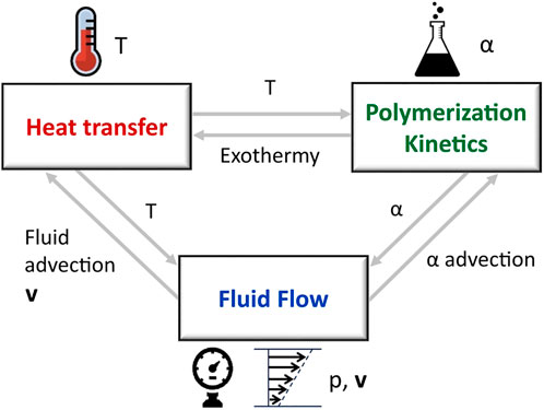
FIGURE 5. Physical sub-models and coupling scheme.

4.2 Assumptions and global implementation

Two simulation steps were performed, similar to the steps in the capillary rise experimental setup:

• Step 1: Pre-heating. The sample is heated by the mold, in the air, until equilibrium is achieved. This step was performed as a stationary study in COMSOL, with only the heat transfer sub-model activated, neglecting the advection of the air inside the porous bar.

• Step 2: Capillary rise. The air is replaced in the tank area by the ambient temperature resin; the simulation starts with initial temperature conditions taken from the result of Step 1 in the bar. Step 2 was performed as a time-dependent study in the software.

Table 1 presents the equations, hypotheses, and material properties introduced in the previous section that were used for Step 2 (capillary rise), using the sub-models presented in Figure 5. The implementation of the couplings between the three physical components is revealed. The initial and boundary conditions, as well as the definition domains, are presented in Figures 6, 7. The heat transfer sub-model was defined over the entire domain, including the material in the tank (air or resin). To simplify the calculations, movement and polymerization of the resin in the tank were treated as negligible. Consequently, the fluid flow sub-model was defined only in the fluid in the porous bar, and the polymerization kinetics sub-model only in the resin in the bar.

TABLE 1

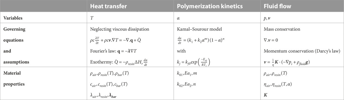
TABLE 1. Assumptions, governing equations, and material properties used for the capillary rise step in the simulation.

FIGURE 6

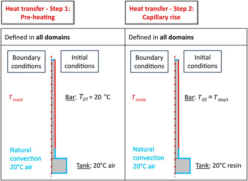
FIGURE 6. Definition domain and initial and boundary conditions for heat transfer in each of the two steps of the simulation.

FIGURE 7

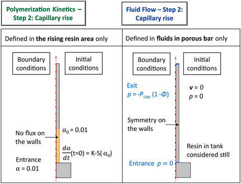
FIGURE 7. Definition domain and initial and boundary conditions for polymerization kinetics and fluid flow during the capillary rise step of the simulation. K–S stands for the previously presented Kamal–Sourour model (Eq. 11).

4.3 Capillary pressure implementation

As mentioned in Figure 7, capillary pressure was implemented as the exit boundary condition at the top of the bar. To ensure that the pressure −P_cap(T) (defined in Eq. 10) was applied at the flow front, the boundary condition BC_exit applied at the exit of the porous bar could be expressed as:

$B{C}_{\mathit{exit}}=-P_{\mathit{cap}}\left(T_{\mathit{mold}}\right)\left(1-\varphi \right)(21)$

where T_mold is the temperature of the mold and ϕ the level-set function defined in section 4.4. Initially, capillary pressure was calculated for the temperature of the front at each time-step. This approach resulted in a rather heavy calculation burden for a negligible difference in results, as the temperature at the flow front very quickly becomes equal to the mold temperature. Therefore, the choice was made to move directly to calculation of capillary pressure at the temperature of the mold. The pressure profile obtained is plotted in Figure 8, in which the experimental pressure profile is compared to the profile obtained on COMSOL. The profile generated via simulation is thus satisfactory in the impregnated area, which is the most important in accurately reproducing the impregnation process. This illustration also shows that capillary pressure is applied at the moving front.

FIGURE 8

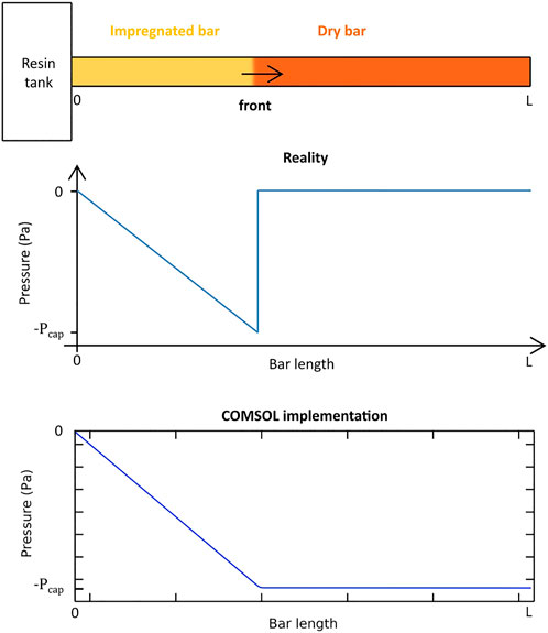
FIGURE 8. Pressure profile during capillary rise in reality and in the COMSOL implementation.

4.4 Level-set method (flow tracking and updating of material properties)

The level-set method was selected to update the material properties according to the macroscopic flow front position at each time-step. The level-set function ϕ returns a value of 1 in impregnated areas and 0 in unimpregnated regions. The principle is presented in Figure 9.

FIGURE 9

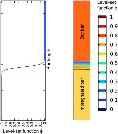
FIGURE 9. Level-set function ϕ and identification of the resin/air interface at ϕ = 0.5.

The level-set model node in COMSOL was used to add the following transport equation (with options to define the associated level-set parameters and the velocity field):

$\frac{\partial \varphi }{\partial t}+\mathit{v}\mathrm{\nabla }\varphi =\gamma \mathrm{\nabla }.\left({ϵ}_{ls}\mathrm{\nabla }\varphi -\varphi \left(1-\varphi \right)\frac{\mathrm{\nabla }\varphi }{|\mathrm{\nabla }\varphi |}\right)(22)$

with γ representing the reinitialization parameter (unit: m/s), ϵ_ls the parameter controlling interface thickness, and v the fluid velocity field (Section 2.2.2). This is the velocity at which the level-set function is transported through advection.

The conditional function if (Boolean, value if Boolean is true, value if Boolean is false), combined with the level-set function, enabled the definition of the material properties of the homogenized copper bar, according to impregnation status:

${\rho }_{\mathit{bar}}\left(T\right)=\text{if}\left(\varphi <0.5,\rho \left({\rho }_{\mathit{air}}\right),\rho \left({\rho }_{\mathit{resin}}\left(T\right)\right)\right)(23)$

$c_{\mathit{bar}}\left(T\right)=\text{if}\left(\varphi \right.<0.5,c\left({\rho }_{\mathit{air}},c\left({\rho }_{\mathit{air}},c_{\mathit{air}}\right),c\left({\rho }_{\mathit{resin}},c_{\mathit{resin}}\left(T\right)\right)\right)(24)$

${\mathit{\lambda }}_{\mathit{bar}}=\left(\begin{array}{cc}\hfill \text{if}\left(\varphi <0.5,{\lambda }_{\perp }\left({\lambda }_{\mathit{air}}\right),{\lambda }_{\perp }\left({\lambda }_{\mathit{resin}}\right)\right)\hfill & \hfill 0\hfill \\ \hfill 0\hfill & \hfill \text{if}\left(\varphi <0.5,{\lambda }_{//}\left({\lambda }_{\mathit{air}}\right),{\lambda }_{//}\left({\lambda }_{\mathit{resin}}\right)\right)\hfill \end{array}\right)(25)$

The relevant properties (Eqs 13–20) were implemented as analytical functions in COMSOL Multiphysics for use when needed. For numerical stability reasons, viscosity was capped (η_capped = 10 × η_ini) for conditions approaching gelation in order to avoid infinite values.

5 Results

The results are given for three temperatures, T_mold = {20, 60, 120}°C.

5.1 Step 1: Pre-heating

The first pre-heating step was stationary. During this step, the mold pre-heats the sample, which is not yet in contact with the resin; therefore, the tank is treated as being filled with air during this step. The obtained equilibria for each mold temperature are presented in Figure 10A.

FIGURE 10

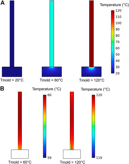
FIGURE 10. Temperature fields for three temperatures (T_mold = {20, 60, 120}°C) after Step 1 (pre-heating), plotted (A) on a 20°C–120°C scale, and (B) on a finer scale.

At this temperature scale, no heat gradient is visible in the porous bar, indicating that the mold efficiently conducts heat to the bar. The delimitation is more visible at a more fine-grained temperature scale (Figure 10B). The effects of the natural convection of air at the bottom of the bar and at the very top of the bar are visible. Additionally, a small gradient is present in the lateral direction, indicating that the mold is heating the sides of the bar slightly more than the center, which seems consistent with the boundary conditions implemented. However, the global temperature difference is very small (less than 1°C).

5.2 Step 2: Capillary rise

5.2.1 Capillary rise results

The second step of the simulation was anisothermal reactive capillary rise. The average height of the flow front obtained was extracted and compared to the experimental data for the three mold temperatures simulated (Figure 11). The results of the analytical model from Figure 2 for 20°C are also plotted for comparison.

FIGURE 11

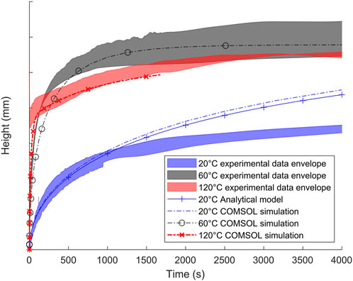
FIGURE 11. Comparison of experimental data and COMSOL capillary rise simulation at 20, 60, and 120°C.

The COMSOL simulation was found to fit well with the previous analytical model at 20°C. This validates the implementation in this case, with negligible polymerization at ambient temperature, as confirmed by Figure 12. Similarly, in the 60°C case, the simulation was found to fit well with the experimental data, presenting a very similar match to that previously obtained.

FIGURE 12

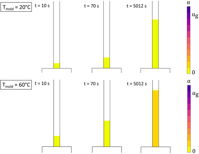
FIGURE 12. Advancement fields for T_mold = 20°C and 60°C at three time-steps.

For the 60°C and 120°C cases, both the analytical model and the simulation slightly underestimated the capillary rise velocity during the first few hundred seconds. At 120°C, in contrast with the previous analytical model, the sudden change of regime that is visible in the experimental data also occurs in the simulation. This indicates that the full set of coupling and modeling choices made was effective in reproducing the relevant phenomena. In this high-temperature case, calculation ended at around 1700 s due to numerical instabilities in the fluid flow sub-model, which was difficult to run with ongoing polymerization generating high viscosities and drastically reducing the velocity of the resin.

5.2.2 Temperature, advancement, and viscosity field results

The polymerization advancement and filling fields were plotted at three time-steps for the first two cases, i.e., for the 20°C and 60°C molds (Figure 12). Notably, the higher initial speed of impregnation at 60°C compared to 20°C is clearly visible in these figures. The advancement scale is extended to a value only slightly above α_g to enable illustration of small evolutions and the gelation transition (which occurs when the system approaches the α_g conversion). At 20°C, the thermosetting resin was not found to react at all, which is consistent. At 60°C, the reaction was extremely slow, reaching only a small degree of conversion at the end of the simulated capillary rise, far below the advancement at gelation (α_g).

Temperature, advancement, and viscosity fields during capillary rise are presented and analyzed for the 120°C mold case at three different time-steps (Figure 13). First, regarding the temperature fields, the white line represents the flow front for each printed time step. The delimitation of the mold at the bottom of the bar is visible, lowering the temperature because of the natural convection of the air. The arrival of the resin cools the bottom of the bar slightly, amplifying the effect of the natural external convection. However, the amplitude of the cooling witnessed at t = 3 s is very small compared to the amplitude of pre-heating (Figure 10), with a minimum value of 118°C. The impact dissipates after only 70 s, the resin flow being slower and its temperature being homogenized with that of the porous bar.

FIGURE 13

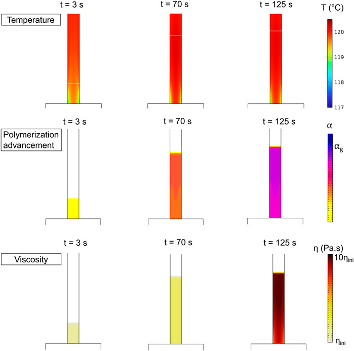
FIGURE 13. Temperature, advancement, and viscosity fields for T_mold = 120°C at three time-steps.

After some time, the resin warms up in the center of the bar (0.2°C above the mold temperature, as illustrated in the images for t = 70 and 125 s): the impact of the exothermy of the reaction on the temperature seems to be greater in the center than at the sides of the porous bar in contact with the mold.

Second, the advancement fields are plotted in parallel for the same time-steps. Flow front movement over time is visible, and the increase in conversion can also be observed; advancement reaches a value close to α_g after 125 s. Spatially, the advancement rise starts at the top of the center of the impregnated area, then grows and spreads to the bottom. Finally, viscosity evolution is presented. Between 3 and 70 s, a very small viscosity rise is visible. At 125 s, a rapid rise occurs, with initial viscosity multiplied 10-fold. Gelation begins in the center of the bar, with less viscous resin that it remains on the sides.

5.2.3 Velocity field results

The pattern of viscosity variation described above implies that it became increasingly difficult for the fluid to rise over time. Curves representing the vertical velocity of the fluid (v_//) are plotted in Figure 14. Initially, velocity is homogeneous and rather high in the entire impregnated area at the beginning of the capillary rise. After 70 s, the fluid has already slowed down, as illustrated in the capillary rise curves, and the first gradient is visible at the top of the center of the area. At 125 s, velocity has fallen globally, and the field is no longer homogeneous: the resin in the center of the bar has slowed down to a greater extent than resin at the sides of the bar.

FIGURE 14

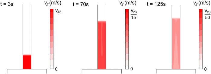
FIGURE 14. Vertical velocity fields for T_mold = 120°C at three time-steps.

6 Discussion

The phenomena competing in the impregnation process are capillary, viscous, and gravitational forces. To analyze the results of simulating capillary rise more deeply, dimensionless numbers can be examined. First, the capillary number Ca can be used to compare the viscous and capillary effects:

$Ca=\frac{v\eta }{\sigma }(26)$

with v representing the velocity of the resin, η its viscosity, and σ the resin/air surface tension. This number was evaluated for each of the three temperatures, neglecting curing. The time points after which Ca fell below 1 were 90 s, 10 s, and 1 s for 20, 60, and 120°C, respectively. This indicates that capillary forces surpass viscous forces increasingly quickly as the temperature rises.

Second, the Reynolds number Re can be used to compare the inertial and viscous effects:

$Re=\frac{\rho v{r}_{\mathit{cap}}}{\eta }(27)$

with ρ representing the density of the resin and r_cap the equivalent capillary radius, reflecting the characteristic size of the system. This number was similarly evaluated for each of the three temperatures, neglecting curing. The time points after which Re fell below 1 were 0, 7, and 90 s for 20, 60, and 120°C, respectively. This indicates that viscous forces take an increasingly long time to exceed inertial forces as the temperature rises. This finding might represent an element of the explanation for the small gap between the simulation and the experimental results at the beginning of the rise in the 60°C and 120°C cases. The goal of this study was to obtain a characterization and simulation of the phenomena on a long timescale, continuing the simulation until equilibrium. Additionally, the experimental method limited the analysis, as data points were available only every 0.5 s. A simulation at a smaller timescale, therefore, would probably require inertial effects to be taken into account.

Finally, the choice to neglect the dynamic contact angle and use the static angle can also be discussed. For Fries and Dreyer (2008), taking the static value seems to have been effective, while Bico (2000) uses a dynamic contact angle model for successful correction of his capillary rise model. Taking an intermediate approach, Pillai and Advani (1996) choose to use an advancing contact angle value, measured for a given speed close to that observed during experiments. Globally, if the fluid is progressing into a capillary, taking the advancing contact angle into account will result in computing a slightly slower capillary rise. Consequently, the choice to prioritize only static contact angles seems relevant in this case: including an advancing contact angle in the first stages of the capillary rise would degrade the correspondence between the simulation results and the experimental data. Once again, such measurements could be needed for capillary rise recordings on a shorter timescale, with higher rates of weight acquisition on the balance.

7 Conclusion

A simulation of the reactive anisothermal capillary rise was implemented, with an anisotropic 2D axisymmetric homogenized domain, coupling heat transfer (neglecting viscous dissipation and taking into account the polymerization exothermy), polymerization kinetics (with a Kamal–Sourour model), and fluid flow (with a Darcy-type flow equation, a Gebart model of permeability, and a modified Castro and Macosko model for the viscosity of the resin). In the cases of 20°C and 60°C molds, the simulation gave very similar results to the analytical model optimized previously (Moisy et al., 2022), confirming that the implementation was correct and suggesting that polymerization played a minor role at these temperatures. In the case of the 120°C mold, the sudden change of regime observed during experimental tests was reproduced by the simulation, meaning that it produced better results than the analytical model. The first objective of this paper was therefore achieved, since the modeling choices made for the simulation enabled the reproduction of the system’s behaviors at 20°C and 60°C and of the change of regime observed at 120°C.

Additionally, subsequent analysis of the results in terms of temperature, advancement, and fluid flow has provided an understanding of the physical mechanisms occurring during this regime change:

• The reaction exothermy heats the bar;

• The heat is evacuated by conduction to a greater extent at the sides of the bar, and less easily in the center, creating a transverse temperature gradient;

• This temperature gradient causes a conversion of reaction gradient, in turn generating an exothermy gradient;

• Gelation starts earlier in the center of the bar than on the sides due to the gradient of advancement, raising the viscosity of the fluid more quickly in the center than at the sides;

• The fluid slows down in the center and flows slightly more quickly at the sides during the transition, creating a velocity gradient in the bar.

Consequently, the second objective of understanding the mechanisms and physical interactions that temporally and spatially explain the macroscopic change of regime observed at 120°C has also been achieved. Future work to pursue this investigation further will be to scale up and complexify the sample geometry, both for experimental trials and in the simulation, in order to make it closer to that of the real rotor (which is around twice the size of the current sample in all directions and includes curved coil regions). This will impose both experimental and simulation-related challenges. In a large rotor, the physical gradients are potentially amplified relative to those observed the sample tested in this study: understanding these will help with developing an understanding of the complexity of the wound rotor impregnation process.

Data availability statement

The datasets presented in this article are not readily available because of industrial confidentiality. Requests to access the datasets should be directed to amelie.moisy@ec-nantes.fr.

Author contributions

AM performed the experimental, modeling, and simulation work and wrote the manuscript. SC-C, ND, PG, and JK provided advice, participated in discussions, and proof-read the manuscript.

Funding

The authors acknowledge the ANRT (Association Nationale Recherche Technologie) for partial funding of this study under the CIFRE program (2019/0089).

Conflict of interest

AM, PG and JK were employed by Renault.

The remaining authors declare that the research was conducted in the absence of any commercial or financial relationships that could be construed as a potential conflict of interest.

Publisher’s note

All claims expressed in this article are solely those of the authors and do not necessarily represent those of their affiliated organizations, or those of the publisher, the editors and the reviewers. Any product that may be evaluated in this article, or claim that may be made by its manufacturer, is not guaranteed or endorsed by the publisher.

References

Advani, S. G., and Sozer, E. M. (2010). Process modeling in composites manufacturing. Boca Raton: CRC Press.

Google Scholar

Ahn, K., Seferis, J., and Berg, J. C. (1997). Simultaneous measurements of permeability and capillary pressure of thermosetting matrices in woven fabric reinforcements. Polym. Compos. 12, 146–152. doi:10.1002/pc.750120303

CrossRef Full Text | Google Scholar

Bico, J. (2000). “Mécanismes d’imprégnation: Surfaces texturées, bigouttes, poreux,” (Paris. Ph.D. thesis.

Google Scholar

Bico, J., and Quéré, D. (2002). Rise of liquids and bubbles in angular capillary tubes. J. colloid Interface Sci. 247, 162–166. doi:10.1006/jcis.2001.8106

PubMed Abstract | CrossRef Full Text | Google Scholar

Bories, S., Mojtabi, A., Prat, M., and Quintard, M. (2008). Transferts de chaleur dans les milieux poreux - changement de phase. Tech. l’ingénieur8251, 1–14.

CrossRef Full Text | Google Scholar

Cai, J., Chen, Y., Liu, Y., Li, S., and Sun, C. (2022). Capillary imbibition and flow of wetting liquid in irregular capillaries: A 100-year review. Adv. Colloid Interface Sci. 304, 102654. doi:10.1016/j.cis.2022.102654

PubMed Abstract | CrossRef Full Text | Google Scholar

Cai, J., Perfect, E., Cheng, C.-L., and Hu, X. (2014). Generalized modeling of spontaneous imbibition based on hagen–Poiseuille flow in tortuous capillaries with variably shaped apertures. Langmuir 30, 5142–5151. doi:10.1021/la5007204

PubMed Abstract | CrossRef Full Text | Google Scholar

Chern, C.-S., and Poehlein, G. (1987). A kinetic model for curing reactions of epoxides with amines. Polym. Eng. Sci. 27, 788–795. doi:10.1002/pen.760271104

CrossRef Full Text | Google Scholar

Chevalier, L., Bruchon, J., Moulin, N., Liotier, P.-J., and Drapier, S. (2018). Accounting for local capillary effects in two-phase flows with relaxed surface tension formulation in enriched finite elements. Comptes Rendus Mécanique 346, 617–633. doi:10.1016/j.crme.2018.06.008

CrossRef Full Text | Google Scholar

Chwastiak, S. (1973). A wicking method for measuring wetting properties of carbon yarns. J. Colloid Interface Sci. 42, 298–309. doi:10.1016/0021-9797(73)90293-2

CrossRef Full Text | Google Scholar

Darcy, H. P. G. (1856). Les Fontaines publiques de la ville de Dijon. Exposition et application des principes à suivre et des formules à employer dans les questions de distribution d’eau. etc (V. Dalamont).

Google Scholar

Fries, N., and Dreyer, M. (2008). An analytic solution of capillary rise restrained by gravity. J. Colloid Interface Sci. 320, 259–263. doi:10.1016/j.jcis.2008.01.009

PubMed Abstract | CrossRef Full Text | Google Scholar

Gebart, B. R. (1992). Permeability of unidirectional reinforcements for RTM. J. Compos. Mater. 26, 1100–1133. doi:10.1177/002199839202600802

CrossRef Full Text | Google Scholar

Hardis, R. (2012). Cure kinetics characterization and monitoring of an epoxy resin for thick composite structures (United States: Iowa State University). Ph.D. thesis.

Ivankovic, M., Incarnato, L., Kenny, J. M., and Nicolais, L. (2003). Curing kinetics and chemorheology of epoxy/anhydride system. J. Appl. Polym. Sci. 90, 3012–3019. doi:10.1002/app.12976

CrossRef Full Text | Google Scholar

Kamal, M. (1973). Integrated thermorheological analysis of the cure of thermosets. SPE Tech. Pap. 19, 187–191.

Google Scholar

Keller, A., Dransfeld, C., and Masania, K. (2016). “Numerical modelling of flow and heat transfer for the compression RTM process with a fast-cure epoxy,” in Book of proceedings of the European Conference of Composites Materials (ECCM17), Germany, June 2016 (Munich ECCM).

Google Scholar

Kubochkin, N., and Gambaryan-Roisman, T. (2022). Capillary-driven flow in corner geometries. Curr. Opin. Colloid and Interface Sci. 59, 101575. doi:10.1016/j.cocis.2022.101575

CrossRef Full Text | Google Scholar

Laplace, P. S. (1806). Supplément au tome 10 de Mécanique céleste (Crapelet).

Google Scholar

Loubeau, F. (2016). Analyse des phénomènes de vieillissement des matériaux d’isolation électrique de machines de traction électrique (France: Université Grenoble Alpes). Ph.D. thesis.

Moisy, A., Comas-Cardona, S., Désilles, N., Genevée, P., and Kolehmainen, J. (2022). “Characterization and modeling of the impregnation process of electric engines’s rotors with a reactive thermosetting resin,” in Proceedings of the 20th European Conference on Composite Materials (ECCM20) 4 - Modeling and Prediction, Lausanne, June 26-30, 2022 (EPFL Lausanne, Composite Construction Laboratory), 405–412. doi:10.5075/epfl-298799/TNQDotTNQ/978-2-9701614-0-0

CrossRef Full Text | Google Scholar

Moragues, M., Nippert, A., Nègre, E., and Blanchard, E. (2021). Moteur électrique: Se réinventer pour conquérir l’automobile. Industrie Technol. 23, 18.

Google Scholar

Nakouzi, S., Pancrace, J., Schmidt, F., Le Maoult, Y., and Berthet, F. (2010). Curing simulation of composites coupled with infrared heating. Int. J. Mater Form. 3, 587–590. doi:10.1007/s12289-010-0838-5

CrossRef Full Text | Google Scholar

Nam, J., and Seferis, J. C. (1993). Application of the kinetic composite methodology to autocatalytic-type thermoset prepreg cures. J. Appl. Polym. Sci. 50, 1555–1564. doi:10.1002/app.1993.070500909

CrossRef Full Text | Google Scholar

Nategh, S., Krings, A., Wallmark, O., and Leksell, M. (2014). Evaluation of impregnation materials for thermal management of liquid-cooled electric machines. IEEE Trans. Industrial Electron. 61, 5956–5965. doi:10.1109/TIE.2014.2308151

CrossRef Full Text | Google Scholar

Nategh, S., Øvrebø, S., Mahdavi, S., and Wallmark, O. (2015). “Thermal modeling of a permanent magnet machine built using litz wire,” in International Conference on Electrical Systems for Aircraft, Railway, Ship Propulsion and Road Vehicles (ESARS), Aachen, 03-05 March 2015 (IEEE), 1. doi:10.1109/ESARS.2015.7101462

CrossRef Full Text | Google Scholar

Ou, H., Sahli, M., Barrière, T., and Gelin, J.-C. (2017). Multiphysics modelling and experimental investigations of the filling and curing phases of bi-injection moulding of thermoplastic polymer/liquid silicone rubbers. Int. J. Adv. Manuf. Technol. 92, 3871–3882. doi:10.1007/s00170-017-0425-8

CrossRef Full Text | Google Scholar

Pillai, K. M., and Advani, S. G. (1996). Wicking across a fiber-bank. J. Colloid Interface Sci. 183, 100–110. doi:10.1006/jcis.1996.0522

CrossRef Full Text | Google Scholar

Sauer, B. B., and Dee, G. T. (1991). Molecular weight and temperature dependence of polymer surface tension: Comparison of experiment with theory. Macromolecules 24, 2124–2126. doi:10.1021/ma00008a070

CrossRef Full Text | Google Scholar

Senecot, J.-m. (2002). Etude de l’imprégnation capillaire de tissus de verre (France: Université de Haute-Alsace). Ph.D. thesis.

Silva, L., Laure, P., Coupez, T., and Digonnet, H. (2016). “Multiphysics for simulation of forming processes,” in Heat transfer in polymer composite materials: Forming processes. Editor N. BOYARD (London: Wiley-ISTE).

CrossRef Full Text | Google Scholar

Simpson, N., Wrobel, R., and Mellor, P. H. (2013). Estimation of equivalent thermal parameters of impregnated electrical windings. IEEE Trans. Industry Appl. 49, 2505–2515. doi:10.1109/TIA.2013.2263271

CrossRef Full Text | Google Scholar

Tucker, C. L., and Dessenberger, R. B. (1994). Governing equations for flow and heat transfer in stationary fiber beds. Compos. Mater. Ser. 35, 257. doi:10.1016/j.compositesa.2004.01.001

CrossRef Full Text | Google Scholar

Wu, S. (1969). Surface and interfacial tensions of polymer melts: I. Polyethylene, polyisobutylene, and polyvinyl acetate. J. Colloid Interface Sci. 31, 153–161. doi:10.1016/0021-9797(69)90321-x

CrossRef Full Text | Google Scholar