A Green’s function-based approach to the concentration tensor fields in arbitrary elastic microstructures

Highlights

• Macrostrains are imposed on elastic material volumes with arbitrary inhomogeneous microstructures.

• Corresponding microstrain distributions are determined in a semi-analytical fashion.

• It involves a homogeneous infinite domain with polarization stress distributions.

• This leads to a Fredholm integral equation involving the elastic Green’s function.

• The solution gives access to homogenized stiffness tensors of arbitrary inhomogeneous microstructures.

1 Introduction–Motivation and scope

The main problem in the wide field of micromechanics of materials (Hill, 1963; Zaoui, 2002) is to quantify the effect of mechanical property distribution throughout the microstructures filling a so-called representative volume element (RVE), on the overall mechanical properties of this RVE, i.e., the properties linking the macroscopic strains (being the average over the microscopic strains inside the RVE) to the macroscopic stresses (being the average over the microscopic stresses inside the RVE). Restricting the present contribution to the case of linear elasticity, the problem comprises the following mathematical relations (Zaoui, 2002):

• geometrical boundary conditions prescribed at the boundary of the RVE, S_RVE, in the form proposed by Hashin (1983)

$\underline{u}\left(\underline{x}\right)=\mathbf{E}\cdot \underline{x},\forall \underline{x}\in S_{\text{RVE}},(1)$

with $\underline{x}$ denoting the microscopic location vector, with $\underline{u}$ denoting the microscopic displacement vector, and with E denoting the macroscopic strain tensor, which is independent of the location $\underline{x}$, see also Table 1. The boundary conditions according to Eq. 1 imply the validity of the strain average rule (Hashin, 1963; Hashin, 1965; Hashin, 1983)

$\mathbf{E}=\frac{1}{V_{\text{RVE}}}\underset{V_{\text{RVE}}}{\int }\mathit{\epsilon }\left(\underline{x}\right)\mathrm{d}V\left(\underline{x}\right)=⟨\mathit{\epsilon }⟩,(2)$

where ɛ denotes the microscopic linearized strain tensors, defined as the symmetric part of the microscopic gradient of the displacement field $u(\underline{x})$, i.e.,

$\begin{array}{ll}\hfill \mathit{\epsilon }\left(\underline{x}\right)& =\frac{1}{2}\left\{{\text{grad}}_x\underline{u}\left(\underline{x}\right)+{\left[{\text{grad}}_x\underline{u}\left(\underline{x}\right)\right]}^T\right\}={\text{grad}}_x^S\underline{u}\left(\underline{x}\right);\hfill \\ \hfill & \forall \underline{x}\in V_{\text{RVE}},\hfill \end{array}(3)$

• the microscopic elastic law being a function of the microstructural position vector $\underline{x}$

$\mathit{\sigma }\left(\underline{x}\right)=\mathbb{c}\left(\underline{x}\right):\mathit{\epsilon }\left(\underline{x}\right),\forall \underline{x}\in V_{\text{RVE}},(4)$

with the microscopic stress tensor σ and the microscopic stiffness tensor $\mathbb{c}$.

• equilibrium conditions

${\underline{\mathrm{\nabla }}}_x\cdot \mathit{\sigma }\left(\underline{x}\right)+\underline{f}\left(\underline{x}\right)=0,\forall \underline{x}\in V_{\text{RVE}},(5)$

where ${\underline{\mathrm{\nabla }}}_x$ stands for the nabla operator and $\underline{f}$ denotes the volume forces;

• the equivalence of macroscopic and microscopic expressions for virtual power densities of internal forces (Jiménez Segura et al., 2022), which, together with Eq. 5, yields the well-known stress average rule as (Hill, 1963; Zaoui, 2002)

$\mathbf{\Sigma }=\frac{1}{V_{\text{RVE}}}\underset{V_{\text{RVE}}}{\int }\mathit{\sigma }\left(\underline{x}\right)\mathrm{d}V\left(\underline{x}\right)=⟨\mathit{\sigma }⟩;(6)$

• the strain concentration (or downscaling) relation linking, in a multilinear way, the macroscopic to the microscopic strain field (Hill, 1963; Zaoui, 2002)

$\mathit{\epsilon }\left(\underline{x}\right)=\mathbb{A}\left(\underline{x}\right):\mathbf{E},\forall \underline{x}\in V_{\text{RVE}},(7)$

where $\mathbb{A}$ is the concentration (or downscaling) tensor;

• the macroscopic elastic law, which follows from Eq. 4 and Eqs. 6, 7 as

$\mathbf{\Sigma }={\mathbb{C}}^{\mathrm{hom}}:\mathbf{E},(8)$

with the homogenized stiffness tensor reading as (Hill, 1963; Zaoui, 2002)

${\mathbb{C}}^{\mathrm{hom}}=\frac{1}{V_{\text{RVE}}}\underset{V_{\text{RVE}}}{\int }\mathbb{c}\left(\underline{x}\right):\mathbb{A}\left(\underline{x}\right)\mathrm{d}V\left(\underline{x}\right).(9)$

The classical approach for making the problem of Eqs. 1–9 tractable is to restrict the discussion to N_r homogeneous subdomains or phases within the RVE. Accordingly, the general microstiffness distribution $\mathbb{c}(\underline{x})$ is replaced by a finite number of microstiffness tensors ${\mathbb{c}}_r,r=1,\dots ,N_r$, which characterize phases of different shapes, typically represented by means of ellipsoids. The strains in the latter are approximated from the solutions of Eshelby’s matrix-inhomogeneity problem (Eshelby, 1957), and combination of these solutions with the strain average rule specified for a finite number of phases leads to the well-known Mori-Tanaka or self-consistent models (Kröner, 1958; Mori and Tanaka, 1973; Benveniste, 1987; Benveniste et al., 1991), with many applications in a variety of disciplines, including construction and biomedical engineering (Bernard et al., 2003; Hellmich et al., 2004; Hellmich and Mang, 2005; Hofstetter et al., 2005; Fritsch and Hellmich, 2007). In this context, we note that composites with inclusions of different shapes and/or orientations may require additional symmetrization steps guaranteeing the existence of an elastic potential (Sevostianov and Kachanov, 2014; Jiménez Segura et al., 2023).

TABLE 1

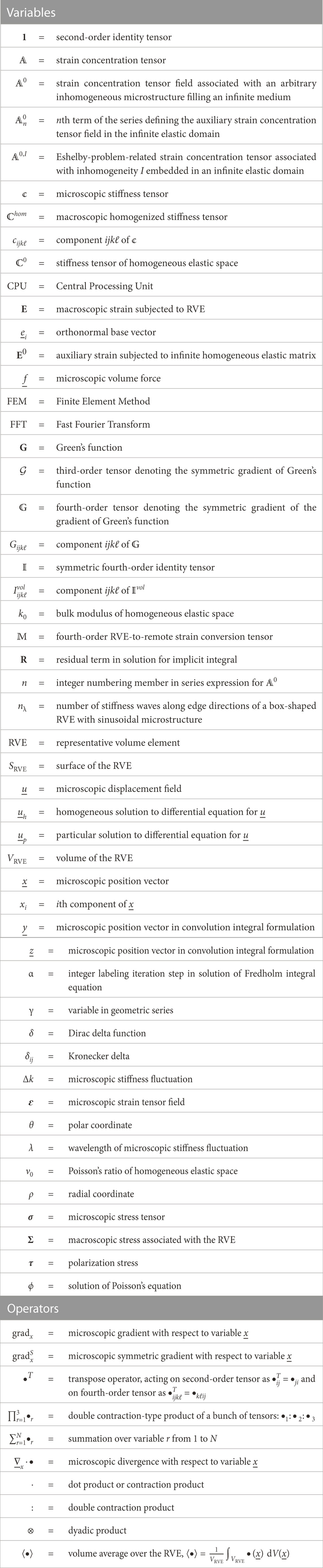
TABLE 1. Mathematical symbols and abbreviations.

Besides this classical approach, it proved useful to introduce, within an RVE, infinitely many (non-spherical) phases, being associated with infinitely many space directions quantified through longitudinal and latitudinal Euler angles, and to associate infinitely many Eshelby problems to each of these directions (Fritsch et al., 2006). After an appropriate discretization of the involved integral expression, the microstrain state within the RVE can be represented sufficiently precisely, so as to allow for upscaling of brittle failure states from the phase-scale, up to the RVE-scale; and this has been shown again for construction and biomedical materials (Fritsch et al., 2009a; Fritsch et al., 2009b; Pichler and Hellmich, 2011; Pichler et al., 2013; Fritsch et al., 2013; Buchner et al., 2022).

Another extension of the classical composite mechanics estimates refers to coated inclusions being embedded in material matrices. A well-known way to approach this problem concerns the extension of Eshelby’s matrix-inclusion problem to a coated inclusion (where the coating may consist of numerous layers, forming an n-layered assemblage (Hervé and Zaoui, 1993; Lipinski et al., 2006)), and then resort to classical combination with the strain average rule, the latter being fed with the inclusion (or core) strains, the layer strains, and the matrix strains. Such models have been very helpful to decipher the mechanical behavior of bone-scaffold composites in tissue engineering (Bertrand and Hellmich, 2009) and of the interfacial transition zone in concrete (Königsberger et al., 2018). Recently, Xu and co-workers proposed a surprisingly simple mathematical alternative to the use of the multiply coated inclusion problem, namely, the repeated use of the Mori-Tanaka estimate, with sequential homogenization of, at a time, one inclusion and one layer playing the role of a matrix; and they successfully applied this strategy to polymer nanocomposites (Xu et al., 2017; Xu et al., 2018), mortar (Xu et al., 2019), and concrete (Xu et al., 2018; Guo et al., 2022).

Still, there is interest in homogenizing over non-uniform stiffness distributions $\mathbb{c}(\underline{x})$; or in other words, over micro-heterogeneous materials with complex microstructures, i.e., such microstructures which cannot be satisfactorily represented by an assemblage of phases as mentioned before. In this context, the most popular approach is based on the Finite Element Method - FEM (Zienkiewicz et al., 2005). It involves discretizing the RVE into very many finite elements, and subjecting it to suitable boundary conditions (Moës et al., 2003; Pahr and Zysset, 2008; Scheiner et al., 2009; Grimal et al., 2011). The latter may be homogeneous, as in Eq. 1, or periodic. This type of analysis, often referred to as computational homogenzation, has been applied to a variety of problems, including woven textures (Moës et al., 2003), bone microstructure (Pahr and Zysset, 2008; Grimal et al., 2011), tissue engineering scaffolds (Scheiner et al., 2009), and fiber-reinforced ultra-high performance concrete (Feng et al., 2022). Corresponding results depend on both the discretization level and the chosen boundary conditions, which requires careful sensitivity analyses to be carried out when aiming at quantitatively reliable results. Also, the computational effort increases with the square of the degrees of freedom, rendering a detailed representation of the microstructure as computationally very expensive. As a remedy to both the discretization and the CPU challenges, FFT-based homogenization schemes based on the Lippmann-Schwinger equation (Lippmann and Schwinger, 1950) have emerged as an interesting alternative to the FEM, in particular so when it comes to image-based computational homogenization (Moulinec and Suquet, 1998; Brisard and Dormieux, 2010; Cai et al., 2019). Such FFT methods are based on a voxel representation of the microstructure, with the elastic properties being constant over one voxel.

Yet, directing our attention back to Eqs. 1–9, we observe that both FEM and FFT-based homogenization techniques primarily focus on the homogenized stiffness tensor ${\mathbb{C}}^{\mathrm{hom}}$, somewhat neglecting the concentration tensor field $\mathbb{A}$. However, the latter quantity, giving access to microsopic stress and strain fields, is of great interest as well, in particular so as concerns upscaling of elasto-brittle material behavior (Fritsch et al., 2009a; Sanahuja et al., 2010; Fritsch et al., 2013; Königsberger et al., 2018; Wolfram et al., 2022), or of eigenstrains and eigenstresses (Levin, 1967; Rosen and Hashin, 1970; Wang et al., 2018).

This motivates the present paper, presenting a novel way to derive strain concentration tensor fields $\mathbb{A}(\underline{x})$, from a given microstiffness distribution $\mathbb{c}(\underline{x})$ characterizing an arbitrary inhomogeneous microstructure. For this purpose, we adopt a key idea underlying the classical phase-based homogenization approaches such as the Mori-Tanaka or the self-consistent scheme, namely, the introduction of an auxiliary problem defined on an infinite elastic domain, and the suitable combination of such an auxiliary problem with the strain average rule of Eq. 2. In this way, we can resort to fundamental elastic solutions in the form of Green’s functions, while also circumventing the rather awkward dependence of homogenization results on the chosen boundary conditions, as encountered with FEM-based computational homogenization approaches. Accordingly, the paper is organized as follows: Section 2 introduces an auxiliary problem on an infinite elastic domain, and its relation to the strain average rule reflecting the geometrical compatibility throughout the microscopically finite RVE. Section 3 covers a Green’s function-based solution to the auxiliary problem of Section 2. Section 4 presents the first Green’s function-based expression of the strain concentration tensor field in an arbitrary inhomogeneous microstructure. After an illustrative example for a microstructure with sinusoidally fluctuating bulk moduli, given in Section 5, and a Discussion in Section 6, the paper is concluded in Section 7.

2 An auxiliary problem on an infinite domain, and its relation to the RVE

Traditional phase-based micromechanical approaches, such as the Mori-Tanaka or the self-consistent estimates, are built on the solution of Eshelby’s matrix-inhomogeneity problem, where an ellipsoidal inhomogeneity of a specific stiffness is embedded into an infinite matrix of yet another stiffness. The latter matrix is remotely subjected to some auxiliary strains E⁰. The solution of Eshelby (1957) then relates the auxiliary strains to the homogeneous strains ɛ^I in the inhomogeneity, according to

${\mathit{\epsilon }}^I={\mathbb{A}}^{0,I}:{\mathbf{E}}^0,(10)$

with ${\mathbb{A}}^{0,I}$ as the concentration tensor associated with inhomogeneity I embedded in an infinite matrix subjected to E⁰. ${\mathbb{A}}^{0,I}$ depends on the stiffness contrast between inhomogeneity and matrix, as well as on the shape of the inhomogeneity and its orientation with respect to the material directions of the matrix. In the traditional approach, ɛ^I is then associated to strains in an ellipsoidal phase inside the RVE, and different inhomogeneities which are all embedded in the same type of matrix are introduced so as to consider different phases within the RVE.

However, as we presently wish to go beyond phase assemblages, we need to extend the auxiliary problem of Eq. 10 beyond homogeneous ellipsoidal domain-related strain ɛ^I and, instead, introduce a general strain field of the form

$\mathit{\epsilon }\left(\underline{x}\right)={\mathbb{A}}^0\left(\underline{x}\right):{\mathbf{E}}^0,(11)$

with ${\mathbb{A}}^0$ as a concentration tensor field associated with an arbitrary inhomogeneous microstructure represented by a stiffness distribution $\mathbb{c}(\underline{x})$, spreading throughout an infinite domain, see Figure 1C. The stiffness distribution is considered as fluctuation around a homogeneous stiffness ${\mathbb{C}}^0$. The strains $\mathit{\epsilon }(\underline{x})$ then consist of two portions: (i) auxiliary strains E⁰ prevailing in the homogeneous infinite domain of stiffness ${\mathbb{C}}^0$, see Figure 1A, and (ii) fluctuations around E⁰ which arise from the fluctuations in the stiffness field, $[\mathbb{c}(\underline{x})-{\mathbb{C}}^0]$, see Figure 1B. These strains can be derived from the Green’s functions known for elastic matrices, together with the concept of polarization stresses introduced by Eshelby, as will be detailed in Section 3. We are left with relating the new auxiliary problem of Eq. 11 to the RVE. Therefore, we consider a finite domain of $\mathbb{c}(\underline{x})$ which is statistically representative of the microstructure within the RVE, we identify the volume of this domain with the volume of the RVE, see Figure 1D, and we then apply the strain average rule of Eq. 2, which yields in combination with Eq. 11 that

$\begin{array}{cc}\hfill & \mathbf{E}=\left[\frac{1}{V_{\text{RVE}}}\underset{V_{\text{RVE}}}{\int }{\mathbb{A}}^0\left(\underline{x}\right)\mathrm{d}V\left(\underline{x}\right)\right]:{\mathbf{E}}^0={\mathbb{M}}^{-1}:{\mathbf{E}}^0\hfill \\ \hfill \Rightarrow & \mathbb{M}={\left[\frac{1}{V_{\text{RVE}}}\underset{V_{\text{RVE}}}{\int }{\mathbb{A}}^0\left(\underline{x}\right)\mathrm{d}V\left(\underline{x}\right)\right]}^{-1},\hfill \end{array}(12)$

with $\mathbb{M}$ as the RVE-to-auxiliary strain conversion tensor. Multiplication from the left, of Eq. 12 with $\mathbb{M}$, and insertion of the corresponding result into Eq. 11, yields

$\mathit{\epsilon }\left(\underline{x}\right)={\mathbb{A}}^0\left(\underline{x}\right):{\left[\frac{1}{V_{\text{RVE}}}\underset{V_{\text{RVE}}}{\int }{\mathbb{A}}^0\left(\underline{x}\right)\mathrm{d}V\left(\underline{x}\right)\right]}^{-1}:\mathbf{E},(13)$

and comparison of Eq. 13 with Eq. 7 yields the strain concentration tensor as

$\mathbb{A}\left(\underline{x}\right)={\mathbb{A}}^0\left(\underline{x}\right):{\left[\frac{1}{V_{\text{RVE}}}\underset{V_{\text{RVE}}}{\int }{\mathbb{A}}^0\left(\underline{x}\right)\mathrm{d}V\left(\underline{x}\right)\right]}^{-1}={\mathbb{A}}^0\left(\underline{x}\right):\mathbb{M},(14)$

and when considering, in addition, Eq. 9, the homogenized stiffness tensor is eventually retrieved as

$\begin{array}{ll}\hfill {\mathbb{C}}^{\mathrm{hom}}& =\left[\frac{1}{V_{\text{RVE}}}\underset{V_{\text{RVE}}}{\int }\mathbb{c}\left(\underline{x}\right):{\mathbb{A}}^0\left(\underline{x}\right)\mathrm{d}V\left(\underline{x}\right)\right]:\hfill \\ \hfill & {\left[\frac{1}{V_{\text{RVE}}}\underset{V_{\text{RVE}}}{\int }{\mathbb{A}}^0\left(\underline{x}\right)\mathrm{d}V\left(\underline{x}\right)\right]}^{-1},\hfill \end{array}(15)$

see Figures 1E, F. Eq. 15 can be reformulated by setting $\mathbb{c}(\underline{x})={\mathbb{C}}^0+\left[\mathbb{c}(\underline{x})-{\mathbb{C}}^0\right]$, which yields

$\begin{array}{ll}\hfill {\mathbb{C}}^{\mathrm{hom}}& ={\mathbb{C}}^0+\left[\frac{1}{V_{\text{RVE}}}\underset{V_{\text{RVE}}}{\int }\left[\mathbb{c}\left(\underline{x}\right)-{\mathbb{C}}^0\right]:{\mathbb{A}}^0\left(\underline{x}\right)\mathrm{d}V\left(\underline{x}\right)\right]:\hfill \\ \hfill & {\left[\frac{1}{V_{\text{RVE}}}\underset{V_{\text{RVE}}}{\int }{\mathbb{A}}^0\left(\underline{x}\right)\mathrm{d}V\left(\underline{x}\right)\right]}^{-1}.\hfill \end{array}(16)$

We are left with the determination of ${\mathbb{A}}^0(\underline{x})$. Therefore, we will first link this property to the elastic Green’s function (Section 3), and provide a Green’s function-based expression of the strain concentration tensor field in an arbitrary inhomogeneous microstructure (Section 4), before giving an illustrative example (Section 5).

FIGURE 1

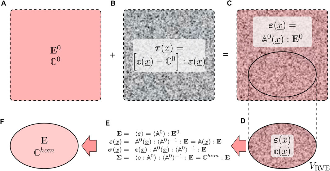
FIGURE 1. Illustration of elements making up the new homogenization scheme: (A) infinite homogeneous elastic matrix of stiffness ${\mathbb{C}}^0$ subjected to background (auxiliary) strains E⁰; (B) same matrix undergoing equilibrated (polarization) stresses which are equivalent to the effect of fluctuations $(\mathbb{c}(\underline{x})-{\mathbb{C}}^0)$ in microstiffness, $\mathbb{c}(\underline{x})$, around the homogeneous stiffness ${\mathbb{C}}^0$, (C) sum of load cases (A) and (B); (D) selection of corresponding microstrains and microstiffnesses within a finite domain (RVE) characterizing the microheterogeneous material; (E) strain averaging over RVE, with $⟨•⟩=\frac{1}{V_{\text{RVE}}}{\int }_{V_{\text{RVE}}}•(\underline{x})\mathrm{d}V(\underline{x})$, and corresponding concentration and homogenization formulae; (F) macroscopic elastic representation of RVE.

3 Green’s function-based solution to the auxiliary problem of the infinite matrix with arbitrary inhomogeneous microelasticity distributions

In order to determine the concentration tensor field ${\mathbb{A}}^0(\underline{x})$ of our new auxiliary problem, we use the method of Green’s functions (Fredholm, 1900; Ting and Lee, 1997). This method is only applicable for homogeneous elastic spaces, which motivates us to adapt a famous idea of Eshelby (1957), which concerns the equivalence of an inhomogeneous elasticity distribution to a homogeneous elastic space subjected to inhomogeneous polarization stresses τ. Mathematically speaking, the constitutive law of Eq. 4 is re-cast into the format (Willis, 1977)

$\mathit{\sigma }\left(\underline{x}\right)={\mathbb{C}}^0:\mathit{\epsilon }\left(\underline{x}\right)+\mathit{\tau }\left(\underline{x}\right).(17)$

Equating Eq. 17 with Eq. 4 yields

$\mathit{\tau }\left(\underline{x}\right)=\left[\mathbb{c}\left(\underline{x}\right)-{\mathbb{C}}^0\right]:\mathit{\epsilon }\left(\underline{x}\right),(18)$

see Figure 1B. Inserting the displacement-to-strain conversion relation of Eq. 3 into the equivalent constitutive law of Eq. 17, followed by inserting the corresponding result into the equilibrium condition of Eq. 5 yields

${\underline{\mathrm{\nabla }}}_x\cdot \left[{\mathbb{C}}^0:{\text{grad}}_x^S\underline{u}\left(\underline{x}\right)\right]=-\left[\underline{f}\left(\underline{x}\right)+{\underline{\mathrm{\nabla }}}_x\cdot \mathit{\tau }\left(\underline{x}\right)\right].(19)$

The solution of the linear partial differential Eq. 19, $\underline{u}(\underline{x})$, is the sum of the homogeneous solution ${\underline{u}}_h$ and the particular solution ${\underline{u}}_p$,

$\underline{u}\left(\underline{x}\right)={\underline{u}}_h\left(\underline{x}\right)+{\underline{u}}_p\left(\underline{x}\right),(20)$

whereby

• the homogeneous solution ${\underline{u}}_h(\underline{x})$ satisfies the homogeneous linear partial differential equation

${\underline{\mathrm{\nabla }}}_x\cdot \left[{\mathbb{C}}^0:{\text{grad}}^S{\underline{u}}_h\left(\underline{x}\right)\right]=0,(21)$

with the inhomogeneous boundary conditions

${\underline{u}}_h\left(\underline{x}\right)={\mathbf{E}}^0\left(\underline{X}\right)\cdot \underline{x},\forall |\underline{x}|\to \infty ;(22)$

• and the particular solution ${\underline{u}}_p(\underline{x})$ satisfies the inhomogeneous linear partial differential equation

${\underline{\mathrm{\nabla }}}_x\cdot \left[{\mathbb{C}}^0:{\text{grad}}^S{\underline{u}}_p\left(\underline{x}\right)\right]=-\left[\underline{f}\left(\underline{x}\right)+{\underline{\mathrm{\nabla }}}_x\cdot \mathit{\tau }\left(\underline{x}\right)\right],(23)$

with homogeneous boundary conditions

${\underline{u}}_p\left(\underline{x}\right)=0,\forall |\underline{x}|\to \infty .(24)$

The homogeneous solution reads as

${\underline{u}}_h\left(\underline{x}\right)={\mathbf{E}}^0\left(\underline{X}\right)\cdot \underline{x},\forall \underline{x}\in {\mathbb{R}}^3.(25)$

The particular solution can be given in the form

${\underline{u}}_p\left(\underline{x}\right)=\underset{{\mathbb{R}}^3}{\int }\mathbf{G}\left(\underline{x}-\underline{y}\right)\cdot \left\{\underline{f}\left(\underline{y}\right)+{\underline{\mathrm{\nabla }}}_y\cdot \mathit{\tau }\left(\underline{y}\right)\right\}\mathrm{d}V\left(\underline{y}\right),(26)$

where $\mathbf{G}(\underline{x}-\underline{y})$ denotes the displacement-related Green’s function tensor, satisfying the differential equation (Kneer, 1965; Ting and Lee, 1997; Tonon et al., 2001; Xie et al., 2016)

${\underline{\mathrm{\nabla }}}_x\cdot \left[{\mathbb{C}}^0:{\text{grad}}_x^S\mathbf{G}\left(\underline{x}-\underline{y}\right)\right]=-\mathbf{1}\delta \left(\underline{x}-\underline{y}\right),(27)$

with boundary conditions

$\mathbf{G}\left(\underline{x}-\underline{y}\right)=0,\forall |\underline{x}|\to \infty .(28)$

In Eq. 27, 1 denotes the second-order identity tensor and δ denotes the Dirac function, with the following properties.

$\delta \left(\underline{x}\right)=0\text{for}\underline{x}\ne 0,(29)$

$\delta \left(\underline{x}\right)=\infty \text{for}\underline{x}=0,(30)$

$\underset{{\mathbb{R}}^3}{\int }\delta \left(\underline{x}\right)\mathrm{d}V\left(\underline{x}\right)=1.(31)$

The last term in Eq. 26 can be transformed by means of the chain rule, the divergence theorem, and the boundary condition given through Eq. 28, yielding

$\underset{{\mathbb{R}}^3}{\int }\mathbf{G}\left(\underline{x}-\underline{y}\right)\cdot {\underline{\mathrm{\nabla }}}_y\cdot \mathit{\tau }\left(\underline{y}\right)\mathrm{d}V\left(\underline{y}\right)=-\underset{{\mathbb{R}}^3}{\int }\left[{\text{grad}}_y\mathbf{G}\left(\underline{x}-\underline{y}\right)\right]:\mathit{\tau }\left(\underline{y}\right)\mathrm{d}V\left(\underline{y}\right).(32)$

Insertion of Eq. 32 into Eq. 26, adding the respective result to Eq. 25, and using the obtained expression $\underline{u}(\underline{x})$ in Eq. 3 yield the microscopic strain field throughout the RVE as

$\mathit{\epsilon }\left(\underline{x}\right)={\mathbf{E}}^0+\underset{{\mathbb{R}}^3}{\int }\mathcal{G}\left(\underline{x}-\underline{y}\right)\cdot \underline{f}\left(\underline{y}\right)\mathrm{d}V\left(\underline{y}\right)-\underset{{\mathbb{R}}^3}{\int }\mathbb{G}\left(\underline{x}-\underline{y}\right):\mathit{\tau }\left(\underline{y}\right)\mathrm{d}V\left(\underline{y}\right).(33)$

In Eq. 33, the following gradients of the Green’s functions were explicitly introduced

$\mathcal{G}\left(\underline{x}-\underline{y}\right)={\text{grad}}_x^S\mathbf{G}\left(\underline{x}-\underline{y}\right),(34)$

$\mathbb{G}\left(\underline{x}-\underline{y}\right)={\text{grad}}_x^S{\text{grad}}_y\mathbf{G}\left(\underline{x}-\underline{y}\right).(35)$

Considering cases where, in Eq. 33, the effect of polarization stresses clearly outweighs that of volume forces, and inserting the polarization stress expression of Eq. 18 into Eq. 33 yields

$\mathit{\epsilon }\left(\underline{x}\right)={\mathbf{E}}^0-\underset{{\mathbb{R}}^3}{\int }\mathbb{G}\left(\underline{x}-\underline{y}\right):\left[\mathbb{c}\left(\underline{y}\right)-{\mathbb{C}}^0\right]:\mathit{\epsilon }\left(\underline{y}\right)\mathrm{d}V\left(\underline{y}\right).(36)$

Eq. 36 is an implicit integral equation for the microscopic strain field, as the latter appears both as a separate term and part of an integrand in a volume integral over the infinite elastic domain. More precisely, the microstrains are the solution of a Fredholm equation of the second kind (Fredholm, 1900). The solution of Eq. 36 is found by means of an infinitely often repeated substitution process concerning $\mathit{\epsilon }(\underline{y})$ in the integral of Eq. 36. Accordingly, the term $\mathit{\epsilon }(\underline{y})$ in the integral of Eq. 36 is numbered in a way reflecting these insertion processes, namely, by $\mathit{\epsilon }({\underline{y}}^{(i)})$, i = 1, 2, …, ∞.

As a starting point, Eq. 36 is specified for $\underline{y}={\underline{y}}^{(1)}$ in the integral of Eq. 36, yielding

$\mathit{\epsilon }\left(\underline{x}\right)={\mathbf{E}}^0-\underset{{\mathbb{R}}^3}{\int }\mathbb{G}\left(\underline{x}-{\underline{y}}^{\left(1\right)}\right):\left[\mathbb{c}\left({\underline{y}}^{\left(1\right)}\right)-{\mathbb{C}}^0\right]:\mathit{\epsilon }\left({\underline{y}}^{\left(1\right)}\right)\mathrm{d}V\left({\underline{y}}^{\left(1\right)}\right).(37)$

In order to come up with an expression for $\mathit{\epsilon }({\underline{y}}^{(1)})$ to be inserted into the integral in Eq. 37, we specify Eq. 37 for ${\underline{y}}^{(1)}={\underline{y}}^{(2)}$ and for $\underline{x}={\underline{y}}^{(1)}$, yielding

$\begin{array}{ll}\hfill \mathit{\epsilon }\left({\underline{y}}^{\left(1\right)}\right)& ={\mathbf{E}}^0-\underset{{\mathbb{R}}^3}{\int }\mathbb{G}\left({\underline{y}}^{\left(1\right)}-{\underline{y}}^{\left(2\right)}\right):\hfill \\ \hfill & \left[\mathbb{c}\left({\underline{y}}^{\left(2\right)}\right)-{\mathbb{C}}^0\right]:\mathit{\epsilon }\left({\underline{y}}^{\left(2\right)}\right)\mathrm{d}V\left({\underline{y}}^{\left(2\right)}\right).\hfill \end{array}(38)$

Insertion of Eq. 38 into Eq. 37 yields

$\begin{array}{ll}\hfill \mathit{\epsilon }\left(\underline{x}\right)& =\left\{\mathbb{I}-\underset{{\mathbb{R}}^3}{\int }\mathbb{G}\left(\underline{x}-{\underline{y}}^{\left(1\right)}\right):\left[\mathbb{c}\left({\underline{y}}^{\left(1\right)}\right)-{\mathbb{C}}^0\right]\mathrm{d}V\left({\underline{y}}^{\left(1\right)}\right)\right\}:{\mathbf{E}}^0\hfill \\ \hfill & +\underset{{\mathbb{R}}^3}{\int }\mathbb{G}\left(\underline{x}-{\underline{y}}^{\left(1\right)}\right):\left[\mathbb{c}\left({\underline{y}}^{\left(1\right)}\right)-{\mathbb{C}}^0\right]:\hfill \\ \hfill & \underset{{\mathbb{R}}^3}{\int }\mathbb{G}\left({\underline{y}}^{\left(1\right)}-{\underline{y}}^{\left(2\right)}\right):\left[\mathbb{c}\left({\underline{y}}^{\left(2\right)}\right)-{\mathbb{C}}^0\right]:\hfill \\ \hfill & \mathit{\epsilon }\left({\underline{y}}^{\left(2\right)}\right)\mathrm{d}V\left({\underline{y}}^{\left(2\right)}\right)\mathrm{d}V\left({\underline{y}}^{\left(1\right)}\right),\hfill \end{array}(39)$

where $\mathbb{I}$ is the symmetric fourth-order identity tensor. We now generalize this idea, in order to come up with the strain field for the (α)-th step of the substitution process, $\mathit{\epsilon }({\underline{y}}^{(\alpha )})$. For this purpose, we specify Eq. 37 for $\underline{x}={\underline{y}}^{(\alpha )}$ and ${\underline{y}}^{(1)}={\underline{y}}^{(\alpha +1)}$. Repeating this process over and over again gives access to a relation involving an auxiliary macrostrain concentration tensor field ${\mathbb{A}}^0(\underline{x})$ and a residual term comprising the implicit strain field $\mathbf{R}[\underline{x},\mathit{\epsilon }({\underline{y}}^{(N)})]$, reading as

$\mathit{\epsilon }\left(\underline{x}\right)={\mathbb{A}}^0\left(\underline{x}\right):{\mathbf{E}}^0+\mathbf{R}\left[\underline{x},\mathit{\epsilon }\left({\underline{y}}^{\left(N\right)}\right)\right].(40)$

In more detail, the concentration tensor field reads as

${\mathbb{A}}^0\left(\underline{x}\right)=\mathbb{I}+\sum _{n=1}^N{\left(-1\right)}^n{\mathbb{A}}_n^0\left(\underline{x}\right),(41)$

where

${\mathbb{A}}_1^0\left(\underline{x}\right)=\underset{{\mathbb{R}}^3}{\int }\mathbb{G}\left(\underline{x}-\underline{y}\right):\left[\mathbb{c}\left(\underline{y}\right)-{\mathbb{C}}^0\right]\mathrm{d}V\left(\underline{y}\right),(42)$

and, for n > 1,

$\begin{array}{ll}\hfill {\mathbb{A}}_n^0\left(\underline{x}\right)& =\underset{{\mathbb{R}}^3}{\int }\dots {\int }_{{\mathbb{R}}^3}\mathbb{G}\left(\underline{x}-{\underline{y}}^{\left(1\right)}\right):\hfill \\ \hfill & \prod _{i=2}^n\left\{\left[\mathbb{c}\left({\underline{y}}^{\left(i-1\right)}\right)-{\mathbb{C}}^0\right]:\mathbb{G}\left({\underline{y}}^{\left(i-1\right)}-{\underline{y}}^{\left(i\right)}\right)\right\}:\hfill \\ \hfill & \left[\mathbb{c}\left({\underline{y}}^{\left(n\right)}\right)-{\mathbb{C}}^0\right]\mathrm{d}V\left({\underline{y}}^{\left(n\right)}\right)\dots \mathrm{d}V\left({\underline{y}}^{\left(1\right)}\right),\hfill \\ \hfill & \forall n\in \left[2,\infty \right).\hfill \end{array}(43)$

The residual term after N iterations reads as

$\begin{array}{ll}\hfill \mathbf{R}\left[\underline{x},\mathit{\epsilon }\left({\underline{y}}^{\left(N\right)}\right)\right]& =\underset{{\mathbb{R}}^3}{\int }\dots \underset{{\mathbb{R}}^3}{\int }\mathbb{G}\left(\underline{x}-{\underline{y}}^{\left(1\right)}\right):\hfill \\ \hfill & \prod _{i=2}^N\left\{\left[\mathbb{c}\left({\underline{y}}^{\left(i-1\right)}\right)-{\mathbb{C}}^0\right]:\mathbb{G}\left({\underline{y}}^{\left(i-1\right)}-{\underline{y}}^{\left(i\right)}\right)\right\}:\hfill \\ \hfill & \left[\mathbb{c}\left({\underline{y}}^{\left(N\right)}\right)-{\mathbb{C}}^0\right]:\mathit{\epsilon }\left({\underline{y}}^{\left(N\right)}\right)\hfill \\ \hfill & \times \mathrm{d}V\left({\underline{y}}^{\left(N\right)}\right)\dots \mathrm{d}V\left({\underline{y}}^{\left(1\right)}\right).\hfill \end{array}(44)$

Note that for N → ∞, $\mathbf{R}[\underline{x},\mathit{\epsilon }({\underline{y}}^{(N)})]\to 0$, provided the following requirement is met:

$\begin{array}{ll}\hfill & \underset{{\mathbb{R}}^3}{\int }{G}_{\mathit{ijk\ell }}\left({\underline{y}}^{\left(\alpha -1\right)}-{\underline{y}}^{\left(\alpha \right)}\right)\left[c_{k\ell mn}\left({\underline{y}}^{\left(\alpha \right)}\right)-C_{k\ell mn}^0\right]\hfill \\ \hfill & \times G_{\mathit{mnpq}}\left({\underline{y}}^{\left(\alpha \right)}-{\underline{y}}^{\left(\alpha +1\right)}\right)\mathrm{d}V\left({\underline{y}}^{\left(\alpha \right)}\right)<1,\forall {\underline{y}}^{\left(\alpha -1\right)},{\underline{y}}^{\left(\alpha +1\right)}\in V_{\text{RVE}},\hfill \end{array}(45)$

for an arbitrary α.

4 Green’s function-based expression of the RVE-related strain concentration tensor field in an arbitrarily inhomogeneous microstructure

After obtaining an analytic expression for the auxiliary strain concentration tensor field ${\mathbb{A}}^0$, see Eq. 41, analytic derivations of the RVE-related quantities are formulated according to Section 2. First, the auxiliary-to-RVE strain concentration follows from Eq. 12. Substitution of $\underline{x}$ by ${\underline{y}}^{(0)}$, which is integrated over the volume of the RVE, V_RVE, (while every other ${\underline{y}}^{(i)}$ is integrated over the entire space, ${\mathbb{R}}^3$), allows for the following expression

$\begin{array}{ll}\hfill \mathbb{M}& =\left[\mathbb{I}+\sum _{n=1}^N\frac{{\left(-1\right)}^n}{V_{\text{RVE}}}\underset{V_{\text{RVE}}}{\int }\underset{{\mathbb{R}}^3}{\int }\dots \underset{{\mathbb{R}}^3}{\int }\prod _{i=1}^n\right.\hfill \\ \hfill & \left\{\mathbb{G}\left({\underline{y}}^{\left(i-1\right)}-{\underline{y}}^{\left(i\right)}\right):\left[\mathbb{c}\left({\underline{y}}^{\left(i\right)}\right)-{\mathbb{C}}^0\right]\right\}\hfill \\ \hfill & \times {\left.\mathrm{d}V\left({\underline{y}}^{\left(n\right)}\right)\dots \mathrm{d}V\left({\underline{y}}^{\left(0\right)}\right)\right]}^{-1}.\hfill \end{array}(46)$

Thus, a comprehenive integral format for the strain concentration tensor field is obtained from inserting Eqs. 41–43 and Eq. 46 into Eq. 14, yielding

$\begin{array}{ll}\hfill \mathbb{A}\left(\underline{x}\right)& =\left[\mathbb{I}-\underset{{\mathbb{R}}^3}{\int }\mathbb{G}\left(\underline{x}-\underline{y}\right):\left[\mathbb{c}\left(\underline{y}\right)-{\mathbb{C}}^0\right]\mathrm{d}V\left(\underline{y}\right)\right.\hfill \\ \hfill & +\sum _{n=2}^N{\left(-1\right)}^n\underset{{\mathbb{R}}^3}{\int }\dots \underset{{\mathbb{R}}^3}{\int }\mathbb{G}\left(\underline{x}-{\underline{y}}^{\left(1\right)}\right):\hfill \\ \hfill & \prod _{i=2}^n\left\{\left[\mathbb{c}\left({\underline{y}}^{\left(i-1\right)}\right)-{\mathbb{C}}^0\right]:\mathbb{G}\left({\underline{y}}^{\left(i-1\right)}-{\underline{y}}^{\left(i\right)}\right)\right\}:\hfill \\ \hfill & \left.\left[\mathbb{c}\left({\underline{y}}^{\left(n\right)}\right)-{\mathbb{C}}^0\right]\mathrm{d}V\left({\underline{y}}^{\left(n\right)}\right)\dots \mathrm{d}V\left({\underline{y}}^{\left(1\right)}\right)\right]:\hfill \\ \hfill & \left[\mathbb{I}+\sum _{n=1}^N\frac{{\left(-1\right)}^n}{V_{\text{RVE}}}\underset{V_{\text{RVE}}}{\int }\underset{{\mathbb{R}}^3}{\int }\dots \underset{{\mathbb{R}}^3}{\int }\prod _{i=1}^n\right.\hfill \\ \hfill & \left\{\mathbb{G}\left({\underline{y}}^{\left(i-1\right)}-{\underline{y}}^{\left(i\right)}\right):\left[\mathbb{c}\left({\underline{y}}^{\left(i\right)}\right)-{\mathbb{C}}^0\right]\right\}\hfill \\ \hfill & \times {\left.\mathrm{d}V\left({\underline{y}}^{\left(n\right)}\right)\dots \mathrm{d}V\left({\underline{y}}^{\left(0\right)}\right)\right]}^{-1}.\hfill \end{array}(47)$

Lastly, the homogenized stiffness tensor, in terms of Green’s functions, is obtained inserting Eq. 47 into Eq. 15. The resulting expression can be simplified by the substitution of $\underline{x}$ by ${\underline{y}}^{(0)}$, yielding

$\begin{array}{ll}\hfill {\mathbb{C}}_{\mathrm{hom}}& ={\mathbb{C}}^0+\left[\frac{1}{V_{\text{RVE}}}\underset{V_{\text{RVE}}}{\int }\left[\mathbb{c}\left({\underline{y}}^{\left(0\right)}\right)-{\mathbb{C}}^0\right]\mathrm{d}V\left({\underline{y}}^{\left(0\right)}\right)+\right.\hfill \\ \hfill & \sum _{n=1}^N\frac{{\left(-1\right)}^n}{V_{\text{RVE}}}\underset{V_{\text{RVE}}}{\int }\underset{{\mathbb{R}}^3}{\int }\dots \underset{{\mathbb{R}}^3}{\int }\prod _{i=1}^n\hfill \\ \hfill & \left\{\left[\mathbb{c}\left({\underline{y}}^{\left(i-1\right)}\right)-{\mathbb{C}}^0\right]:\mathbb{G}\left({\underline{y}}^{\left(i-1\right)}-{\underline{y}}^{\left(i\right)}\right)\right\}:\hfill \\ \hfill & \left.\left[\mathbb{c}\left({\underline{y}}^{\left(n\right)}\right)-{\mathbb{C}}^0\right]\mathrm{d}V\left({\underline{y}}^{\left(n\right)}\right)\dots \mathrm{d}V\left({\underline{y}}^{\left(0\right)}\right)\right]:\hfill \\ \hfill & \left[\mathbb{I}+\sum _{n=1}^N\frac{{\left(-1\right)}^n}{V_{\text{RVE}}}\underset{V_{\text{RVE}}}{\int }\underset{{\mathbb{R}}^3}{\int }\dots \underset{{\mathbb{R}}^3}{\int }\prod _{i=1}^n\right.\hfill \\ \hfill & \left\{\mathbb{G}\left({\underline{y}}^{\left(i-1\right)}-{\underline{y}}^{\left(i\right)}\right):\left[\mathbb{c}\left({\underline{y}}^{\left(i\right)}\right)-{\mathbb{C}}^0\right]\right\}\hfill \\ \hfill & \times {\left.\mathrm{d}V\left({\underline{y}}^{\left(n\right)}\right)\dots \mathrm{d}V\left({\underline{y}}^{\left(0\right)}\right)\right]}^{-1}.\hfill \end{array}(48)$

5 Illustrative example: Microstructure with sinusoidally fluctuating bulk moduli

5.1 Complex microstructure with sinusoidally fluctuating microscopic bulk modulus

In order to illustrate the applicability of the novel integral expressions of Eqs. 41–43, we resort to the Green’s function for an infinitely extended isotropic elastic body with bulk modulus k₀ and Poisson’s ratio ν₀; it reads as (Dvorak, 2012)

$\begin{array}{ll}\hfill \mathbf{G}\left(\underline{x}-\underline{y}\right)& =\frac{\left(1+{\nu }_0\right)}{6\pi k_0\left(1-2{\nu }_0\right)}\mathbf{1}\frac{1}{|\underline{x}-\underline{y}|}\hfill \\ \hfill & -\frac{\left(1+{\nu }_0\right)}{24\pi k_0\left(1-{\nu }_0\right)\left(1-2{\nu }_0\right)}\left({\text{grad}}_x{\text{grad}}_x|\underline{x}-\underline{y}|\right),\hfill \end{array}(49)$

where, with respect to the actual formula (4.5.12) given on page 107 of (Dvorak, 2012), we consider $k_0=\frac{2{\mu }_0(1+{\nu }_0)}{3(1-2{\nu }_0)}$, with μ₀ being the shear modulus. Moreover, we consider a sinusoidal stiffness distribution across this infinitely extended body, according to

$\mathbb{c}\left(\underline{x}\right)={\mathbb{C}}^0+3\mathrm{\Delta }k\text{sin}\left(\frac{2\pi }{{\lambda }_1}{x}_1\right)\text{sin}\left(\frac{2\pi }{{\lambda }_2}{x}_2\right)\text{sin}\left(\frac{2\pi }{{\lambda }_3}{x}_3\right){\mathbb{I}}^{\mathit{vol}},(50)$

where x₁, x₂, and x₃ are the components of location vector $\underline{x}$ with respect to an orthonormal base frame ${\underline{e}}_1$, ${\underline{e}}_2$, ${\underline{e}}_3$, such that $\underline{x}=x_1{\underline{e}}_1+x_2{\underline{e}}_2+x_3{\underline{e}}_3$, and ${\mathbb{I}}^{\mathit{vol}}$ stands for the volumetric part of the symmetric fourth-order unity tensor $\mathbb{I}$. The latter has the components I_ijrs = 1/2 (δ_irδ_js + δ_isδ_jr), while the former reads as ${\mathbb{I}}^{\mathit{vol}}=1/3(\mathbf{1}\otimes \mathbf{1})$, with components $I_{\mathit{ijk\ell }}^{\mathit{vol}}=1/3({\delta }_{ij}{\delta }_{k\ell })$, where 1 is the second-order unity tensor with the Kronecker delta δ_ij as its components. Δk is a parameter which scales the stiffness variance and λ_i sets the size of one fluctuation in direction i.

5.2 Normal strain-related components of ${\mathbb{A}}^0(\underline{x})$

The auxiliary strain downscaling tensor ${\mathbb{A}}^0(\underline{x})$ is the result of the sum of an infinite series, see Eq. 41. The first term of this series, ${\mathbb{A}}_1^0(\underline{x})$, is defined through Eq. 42, so that consideration of Eq. 50 yields the component 1111 of ${\mathbb{A}}_1^0$ as

$\begin{array}{ll}\hfill A_{\mathrm{1,1111}}^0\left(\underline{x}\right)& =\sum _{h=1}^3\sum _{\ell =1}^3\underset{{\mathbb{R}}^3}{\int }{G}_{\mathrm{11}\mathit{h\ell }\mathit{h\ell }}\left(\underline{x}-\underline{y}\right)\left[3\mathrm{\Delta }k\text{sin}\left(\frac{2\pi }{{\lambda }_1}{y}_1\right)\right.\hfill \\ \hfill & \times \left.\text{sin}\left(\frac{2\pi }{{\lambda }_2}{y}_2\right)\text{sin}\left(\frac{2\pi }{{\lambda }_3}{y}_3\right)I_{h\ell 11}^{\mathit{vol}}\right]\mathrm{d}V\left(\underline{y}\right)\hfill \\ \hfill & =\mathrm{\Delta }k\sum _{\ell =1}^3\underset{{\mathbb{R}}^3}{\int }{G}_{11\ell \ell }\left(\underline{x}-\underline{y}\right)\text{sin}\left(\frac{2\pi }{{\lambda }_1}{y}_1\right)\hfill \\ \hfill & \times \text{sin}\left(\frac{2\pi }{{\lambda }_2}{y}_2\right)\text{sin}\left(\frac{2\pi }{{\lambda }_3}{y}_3\right)\mathrm{d}V\left(\underline{y}\right).\hfill \end{array}(51)$

In order to retrieve the components G₁₁₁₁, G₁₁₂₂, and G₁₁₃₃, we start with the general expression for the components of the Green’s function of Eq. 49, reading as

$\begin{array}{ll}\hfill G_{ij}& =\frac{\left(1+{\nu }_0\right)}{6\pi k_0\left(1-2{\nu }_0\right)}\frac{{\delta }_{ij}}{|\underline{x}-\underline{y}|}\hfill \\ \hfill & -\frac{\left(1+{\nu }_0\right)}{24\pi k_0\left(1-{\nu }_0\right)\left(1-2{\nu }_0\right)}\left(\frac{{\partial }^2}{\partial x_i\partial x_j}|\underline{x}-\underline{y}|\right).\hfill \end{array}(52)$

The fourth-order Green’s function gradient according to Eq. 35 exhibits the following components

$\begin{array}{ll}\hfill G_{\mathit{ijk\ell }}& =\frac{\left(1+{\nu }_0\right)}{12\pi k_0\left(1-2{\nu }_0\right)}\left(\frac{{\partial }^2}{\partial x_j\partial y_{\ell }}\frac{{\delta }_{ik}}{|\underline{x}-\underline{y}|}+\frac{{\partial }^2}{\partial x_i\partial y_{\ell }}\frac{{\delta }_{jk}}{|\underline{x}-\underline{y}|}\right)\hfill \\ \hfill & -\frac{\left(1+{\nu }_0\right)}{24\pi k_0\left(1-{\nu }_0\right)\left(1-2{\nu }_0\right)}\left(\frac{{\partial }^4}{\partial x_i\partial x_j\partial x_k\partial y_{\ell }}|\underline{x}-\underline{y}|\right).\hfill \end{array}(53)$

In order to evaluate Eq. 53, it is useful to recall the following properties of the spatial derivatives of the norm $|\underline{x}-\underline{y}|$. The first-order derivative of the aforementioned norm reads as

$\frac{\partial }{\partial x_i}|\underline{x}-\underline{y}|=\frac{x_i-y_i}{|\underline{x}-\underline{y}|},(54)$

revealing the interesting property

$\frac{\partial }{\partial x_i}|\underline{x}-\underline{y}|=-\frac{\partial }{\partial y_i}|\underline{x}-\underline{y}|.(55)$

The first derivative of the inverse of the norm $|\underline{x}-\underline{y}|$ reads as

$\frac{\partial }{\partial x_i}\left(\frac{1}{|\underline{x}-\underline{y}|}\right)=-\frac{x_i-y_i}{|\underline{x}-\underline{y}{|}^3},(56)$

revealing the interesting property

$\frac{\partial }{\partial x_i}\frac{1}{|\underline{x}-\underline{y}|}=-\frac{\partial }{\partial y_i}\frac{1}{|\underline{x}-\underline{y}|}.(57)$

Eq. 55 and Eq. 57 allow for re-writing Eq. 53 as

$\begin{array}{ll}\hfill G_{\mathit{ijk\ell }}& =-\frac{\left(1+{\nu }_0\right)}{12\pi k_0\left(1-2{\nu }_0\right)}\left(\frac{{\partial }^2}{\partial x_j\partial x_{\ell }}\frac{{\delta }_{ik}}{|\underline{x}-\underline{y}|}+\frac{{\partial }^2}{\partial x_i\partial x_{\ell }}\frac{{\delta }_{jk}}{|\underline{x}-\underline{y}|}\right)\hfill \\ \hfill & +\frac{\left(1+{\nu }_0\right)}{24\pi k_0\left(1-{\nu }_0\right)\left(1-2{\nu }_0\right)}\left(\frac{{\partial }^4}{\partial x_i\partial x_j\partial x_k\partial x_{\ell }}|\underline{x}-\underline{y}|\right),\hfill \end{array}(58)$

so that the components occurring in Eq. 51 read as

$\begin{array}{ll}\hfill G_{1111}& =-\frac{\left(1+{\nu }_0\right)}{6\pi k_0\left(1-2{\nu }_0\right)}\left(\frac{{\partial }^2}{\partial x_1^2}\frac{1}{|\underline{x}-\underline{y}|}\right)\hfill \\ \hfill & +\frac{\left(1+{\nu }_0\right)}{24\pi k_0\left(1-{\nu }_0\right)\left(1-2{\nu }_0\right)}\left(\frac{{\partial }^4}{\partial x_1^4}|\underline{x}-\underline{y}|\right),\hfill \end{array}(59)$

$G_{1122}=\frac{\left(1+{\nu }_0\right)}{24\pi k_0\left(1-{\nu }_0\right)\left(1-2{\nu }_0\right)}\left(\frac{{\partial }^4}{\partial x_1^2\partial x_2^2}|\underline{x}-\underline{y}|\right),(60)$

$G_{1133}=\frac{\left(1+{\nu }_0\right)}{24\pi k_0\left(1-{\nu }_0\right)\left(1-2{\nu }_0\right)}\left(\frac{{\partial }^4}{\partial x_1^2\partial x_3^2}|\underline{x}-\underline{y}|\right).(61)$

The sum of Eqs. 59–61, to be calculated in Eq. 51, can be further simplified through an identity which follows from deriving Eq. 54 with respect to the components of the location vector,

$\frac{{\partial }^2}{\partial x_i^2}|\underline{x}-\underline{y}|=\frac{{\sum }_{k\ne i}{\left(x_k-y_k\right)}^2}{|\underline{x}-\underline{y}{|}^3}.(62)$

Namely, Eq. 62 entails the following identity

$\frac{{\partial }^2}{\partial x_1^2}|\underline{x}-\underline{y}|+\frac{{\partial }^2}{\partial x_2^2}|\underline{x}-\underline{y}|+\frac{{\partial }^2}{\partial x_3^2}|\underline{x}-\underline{y}|=2\frac{1}{|\underline{x}-\underline{y}|},(63)$

twofold derivation of which yields an identity comprising the derivatives of the norm $|\underline{x}-\underline{y}|$ occurring in Eqs. 59–61, reading as

$\frac{{\partial }^4}{\partial x_1^4}|\underline{x}-\underline{y}|+\frac{{\partial }^4}{\partial x_1^2\partial x_2^2}|\underline{x}-\underline{y}|+\frac{{\partial }^4}{\partial x_1^2\partial x_3^2}|\underline{x}-\underline{y}|=2\frac{{\partial }^2}{\partial x_1^2}\frac{1}{|\underline{x}-\underline{y}|}.(64)$

Insertion of Eqs. 59–61 into Eq. 51, while considering Eq. 64, yields

$\begin{array}{ll}\hfill A_{\mathrm{1,1111}}^0\left(\underline{x}\right)& =\frac{-\mathrm{\Delta }k\left(1+{\nu }_0\right)}{12\pi k_0\left(1-{\nu }_0\right)}\underset{{\mathbb{R}}^3}{\int }\left(\frac{{\partial }^2}{\partial x_1^2}\frac{1}{|\underline{x}-\underline{y}|}\right)\text{sin}\left(\frac{2\pi }{{\lambda }_1}{y}_1\right)\hfill \\ \hfill & \times \text{sin}\left(\frac{2\pi }{{\lambda }_2}{y}_2\right)\text{sin}\left(\frac{2\pi }{{\lambda }_3}{y}_3\right)\mathrm{d}V\left(\underline{y}\right).\hfill \end{array}(65)$

A change of variable to $\underline{z}=\underline{y}-\underline{x}$ results in

$\begin{array}{ll}\hfill A_{\mathrm{1,1111}}^0\left(\underline{x}\right)& =\frac{-\mathrm{\Delta }k\left(1+{\nu }_0\right)}{12\pi k_0\left(1-{\nu }_0\right)}\underset{{\mathbb{R}}^3}{\int }\left(\frac{{\partial }^2}{\partial z_1^2}\frac{1}{|-\underline{z}|}\right)\hfill \\ \hfill & \times \text{sin}\left[\frac{2\pi }{{\lambda }_1}\left(x_1+z_1\right)\right]\text{sin}\left[\frac{2\pi }{{\lambda }_2}\left(x_2+z_2\right)\right]\hfill \\ \hfill & \times \text{sin}\left[\frac{2\pi }{{\lambda }_3}\left(x_3+z_3\right)\right]\mathrm{d}V\left(\underline{z}\right).\hfill \end{array}(66)$

Transforming Eq. 66 by means of

$\text{sin}\left(a+b\right)=\text{sin}\left(a\right)\text{cos}\left(b\right)+\text{cos}\left(a\right)\text{sin}\left(b\right),(67)$

and considering the second derivative of the inverse of the norm of $-\underline{z}$ as

$\frac{{\partial }^2}{\partial z_1^2}\left(\frac{1}{|-\underline{z}|}\right)=\frac{2{\left(-z_1\right)}^2-{\left(-z_2\right)}^2-{\left(-z_3\right)}^2}{|-\underline{z}{|}^5},(68)$

as well as that the even and odd functions appearing as factors in the integral expression of Eq. 66 imply vanishing integrals

$\underset{-a}{\overset{a}{\int }}\left(\frac{{\partial }^2}{\partial z_1^2}\frac{1}{|-\underline{z}|}\right)\text{sin}\left(\frac{2\pi }{{\lambda }_i}{z}_i\right)\mathrm{d}{z}_i=0,\forall a\in \mathbb{R},i\in \left[\mathrm{1,2,3}\right],(69)$

we arrive at

$\begin{array}{ll}\hfill A_{\mathrm{1,1111}}^0\left(\underline{x}\right)& =\frac{-\mathrm{\Delta }k\left(1+{\nu }_0\right)}{12\pi k_0\left(1-{\nu }_0\right)}\text{sin}\left(\frac{2\pi }{{\lambda }_1}{x}_1\right)\text{sin}\left(\frac{2\pi }{{\lambda }_2}{x}_2\right)\text{sin}\left(\frac{2\pi }{{\lambda }_3}{x}_3\right)\hfill \\ \hfill & \times \underset{{\mathbb{R}}^3}{\int }\left(\frac{{\partial }^2}{\partial z_1^2}\frac{1}{|-\underline{z}|}\right)\text{cos}\left(\frac{2\pi }{{\lambda }_1}{z}_1\right)\hfill \\ \hfill & \times \text{cos}\left(\frac{2\pi }{{\lambda }_2}{z}_2\right)\text{cos}\left(\frac{2\pi }{{\lambda }_3}{z}_3\right)\mathrm{d}V\left(\underline{z}\right).\hfill \end{array}(70)$

Noting that $\frac{\partial }{\partial z_1}\frac{1}{|\underline{z^{\prime }}-\underline{z}|}=-\frac{\partial }{\partial z_1^{\prime }}\frac{1}{|\underline{z^{\prime }}-\underline{z}|}$ and $\frac{{\partial }^2}{\partial z_1^2}\frac{1}{|\underline{z^{\prime }}-\underline{z}|}=\frac{{\partial }^2}{\partial z_1^{\prime 2}}\frac{1}{|\underline{z^{\prime }}-\underline{z}|}$, the integral in Eq. 70 can be expressed by means of an auxiliary function in ${\underline{z}}^{\prime }$, according to

$\begin{array}{ll}\hfill & \underset{{\mathbb{R}}^3}{\int }\left(\frac{{\partial }^2}{\partial z_1^2}\frac{1}{|\underline{-z}|}\right)\text{cos}\left(\frac{2\pi }{{\lambda }_1}{z}_1\right)\text{cos}\left(\frac{2\pi }{{\lambda }_2}{z}_2\right)\text{cos}\left(\frac{2\pi }{{\lambda }_3}{z}_3\right)\mathrm{d}V\left(\underline{z}\right)\hfill \\ \hfill & =\frac{{\partial }^2\varphi }{\partial z_1^{\prime 2}}\left({\underline{z}}^{\prime }=0\right),\hfill \end{array}(71)$

where the auxiliary function $\varphi ({\underline{z}}^{\prime })$ stands for

$\varphi \left({\underline{z}}^{\prime }\right)=\underset{{\mathbb{R}}^3}{\int }\frac{1}{|\underline{z^{\prime }}-\underline{z}|}\text{cos}\left(\frac{2\pi }{{\lambda }_1}{z}_1\right)\text{cos}\left(\frac{2\pi }{{\lambda }_2}{z}_2\right)\text{cos}\left(\frac{2\pi }{{\lambda }_3}{z}_3\right)\mathrm{d}V\left(\underline{z}\right).(72)$

Eq. 72 exhibits two remarkable properties. Firstly, its format

$\varphi \left({\underline{z}}^{\prime }\right)=\underset{{\mathbb{R}}^3}{\int }\frac{1}{|\underline{z^{\prime }}-\underline{z}|}f\left(\underline{z}\right)\mathrm{d}V\left(\underline{z}\right)(73)$

is the solution of the Poisson’s equation

${\mathrm{\nabla }}^2\varphi \left({\underline{z}}^{\prime }\right)=-4\pi f\left({\underline{z}}^{\prime }\right).(74)$

Secondly, Eq. 72 is symmetric in the sense of

$\begin{array}{lll}\hfill \varphi \left(z_1^{\prime },z_2^{\prime },z_3^{\prime }\right)& =\varphi \left(z_1^{\prime },z_3^{\prime },z_2^{\prime }\right)=\varphi \left(z_2^{\prime },z_3^{\prime },z_1^{\prime }\right)=\varphi \left(z_2^{\prime },z_1^{\prime },z_3^{\prime }\right)\hfill & \hfill \\ \hfill & =\varphi \left(z_3^{\prime },z_1^{\prime },z_2^{\prime }\right)=\varphi \left(z_3^{\prime },z_2^{\prime },z_1^{\prime }\right)\hfill & \hfill \\ \hfill & \to \frac{\partial \varphi }{\partial z_1^{\prime }}=\frac{\partial \varphi }{\partial z_2^{\prime }}=\frac{\partial \varphi }{\partial z_3^{\prime }}\hfill & \hfill \\ \hfill & \to \frac{{\partial }^2\varphi }{\partial z_1^{\prime 2}}=\frac{{\partial }^2\varphi }{\partial z_2^{\prime 2}}=\frac{{\partial }^2\varphi }{\partial z_3^{\prime 2}}.\hfill & \hfill \end{array}(75)$

Use of the latter relations in Eq. 74, while accounting for the structure of f according to Eq. 72 and Eq. 73, yields

${\mathrm{\nabla }}^2\varphi \left({\underline{z}}^{\prime }\right)=3\frac{{\partial }^2\varphi }{\partial z_1^{\prime 2}}=-4\pi \text{cos}\left(\frac{2\pi }{{\lambda }_1}{z}_1^{\prime }\right)\text{cos}\left(\frac{2\pi }{{\lambda }_2}{z}_2^{\prime }\right)\text{cos}\left(\frac{2\pi }{{\lambda }_3}{z}_3^{\prime }\right),(76)$

where we made use of Eq. 75. Solving the equation for $\frac{{\partial }^2\varphi }{\partial z_1^{\prime 2}}({\underline{z}}^{\prime }=0)$ and inserting the corresponding result into Eq. 70 yield

$A_{\mathrm{1,1111}}^0\left(\underline{x}\right)=\frac{1}{3}\left[\frac{\mathrm{\Delta }k\left(1+{\nu }_0\right)}{3k_0\left(1-{\nu }_0\right)}\right]\text{sin}\left(\frac{2\pi }{{\lambda }_1}{x}_1\right)\text{sin}\left(\frac{2\pi }{{\lambda }_2}{x}_2\right)\text{sin}\left(\frac{2\pi }{{\lambda }_3}{x}_3\right).(77)$

The second term of the series for the auxiliary concentration tensor for the considered sinusoidal isotropic micro-stiffness distribution follows from insertion of Eq. 50 into Eq. 43, so that its component 1111 is obtained as

$\begin{array}{ll}\hfill A_{\mathrm{2,1111}}^0\left(\underline{x}\right)& =\sum _{h=1}^3\sum _{\ell =1}^3\sum _{i=1}^3\sum _{j=1}^3\underset{{\mathbb{R}}^3}{\int }\underset{{\mathbb{R}}^3}{\int }{G}_{\mathit{11h\ell }}\left(\underline{x}-\underline{y}\right)\hfill \\ \hfill & \times \left[3\mathrm{\Delta }k\text{sin}\left(\frac{2\pi }{{\lambda }_1}{y}_1\right)\text{sin}\left(\frac{2\pi }{{\lambda }_2}{y}_2\right)\text{sin}\left(\frac{2\pi }{{\lambda }_3}{y}_3\right)I_{h\ell ij}^{\mathit{vol}}\right]\hfill \\ \hfill & \times \sum _{m=1}^3\sum _{n=1}^3{G}_{\mathit{ijmn}}\left(\underline{y}-\underline{y^{\prime }}\right)\hfill \\ \hfill & \times \left[3\mathrm{\Delta }k\text{sin}\left(\frac{2\pi }{{\lambda }_1}{y}_1^{\prime }\right)\text{sin}\left(\frac{2\pi }{{\lambda }_2}{y}_2^{\prime }\right)\right.\hfill \\ \hfill & \times \left.\text{sin}\left(\frac{2\pi }{{\lambda }_3}{y}_3^{\prime }\right)I_{mn11}^{\mathit{vol}}\right]\mathrm{d}V\left(\underline{y^{\prime }}\right)\mathrm{d}V\left(\underline{y}\right).\hfill \end{array}(78)$

Specification of Eq. 78 for Eq. 58, while considering the identity of Eq. 64, yields

$\begin{array}{ll}\hfill A_{\mathrm{2,1111}}^0\left(\underline{x}\right)& ={\left[\frac{-\mathrm{\Delta }k\left(1+{\nu }_0\right)}{12\pi k_0\left(1-{\nu }_0\right)}\right]}^2\underset{{\mathbb{R}}^3}{\int }\left(\frac{{\partial }^2}{\partial x_1^2}\frac{1}{|\underline{x}-\underline{y}|}\right)\hfill \\ \hfill & \times \text{sin}\left(\frac{2\pi }{{\lambda }_1}{y}_1\right)\text{sin}\left(\frac{2\pi }{{\lambda }_2}{y}_2\right)\text{sin}\left(\frac{2\pi }{{\lambda }_3}{y}_3\right)\hfill \\ \hfill & \times {\mathrm{\nabla }}^2\left[\underset{{\mathbb{R}}^3}{\int }\left(\frac{1}{|\underline{y}-{\underline{y}}^{\prime }|}\right)\text{sin}\left(\frac{2\pi }{{\lambda }_1}{y}_1^{\prime }\right)\right.\hfill \\ \hfill & \left.\times \text{sin}\left(\frac{2\pi }{{\lambda }_2}{y}_2^{\prime }\right)\text{sin}\left(\frac{2\pi }{{\lambda }_3}{y}_3^{\prime }\right)\mathrm{d}V\left({\underline{y}}^{\prime }\right)\right]\mathrm{d}V\left(\underline{y}\right).\hfill \end{array}(79)$

Considering the last integral in Eq. 79 as the Green’s function solving the Poisson’s equation

${\mathrm{\nabla }}^2\varphi \left(\underline{y}\right)=-4\pi \text{sin}\left(\frac{2\pi }{{\lambda }_1}{y}_1\right)\text{sin}\left(\frac{2\pi }{{\lambda }_2}{y}_2\right)\text{sin}\left(\frac{2\pi }{{\lambda }_3}{y}_3\right)(80)$

yields

$\begin{array}{ll}\hfill A_{\mathrm{2,1111}}^0\left(\underline{x}\right)& =\left(-4\pi \right){\left[\frac{-\mathrm{\Delta }k\left(1+{\nu }_0\right)}{12\pi k_0\left(1-{\nu }_0\right)}\right]}^2\underset{{\mathbb{R}}^3}{\int }\left(\frac{{\partial }^2}{\partial x_1^2}\frac{1}{|\underline{x}-\underline{y}|}\right)\hfill \\ \hfill & \times {\text{sin}}^2\left(\frac{2\pi }{{\lambda }_1}{y}_1\right){\text{sin}}^2\left(\frac{2\pi }{{\lambda }_2}{y}_2\right){\text{sin}}^2\left(\frac{2\pi }{{\lambda }_3}{y}_3\right)\mathrm{d}V\left(\underline{y}\right).\hfill \end{array}(81)$

Recalling from Eq. 65 and Eq. 77 that

$\underset{{\mathbb{R}}^3}{\int }\left(\frac{{\partial }^2}{\partial x_1^2}\frac{1}{|\underline{x}-\underline{y}|}\right)f\left(\underline{y}\right)\mathrm{d}V\left(\underline{y}\right)=-\frac{4\pi }{3}f\left(\underline{x}\right),(82)$

for any $f(\underline{y})$ with the symmetry properties of Eq. 75, the integral in Eq. 81 can be solved, yielding

$\begin{array}{ll}\hfill A_{\mathrm{2,1111}}^0\left(\underline{x}\right)& =\frac{1}{3}{\left[\frac{\mathrm{\Delta }k\left(1+{\nu }_0\right)}{3k_0\left(1-{\nu }_0\right)}\right]}^2{\text{sin}}^2\left(\frac{2\pi }{{\lambda }_1}{x}_1\right)\hfill \\ \hfill & \times {\text{sin}}^2\left(\frac{2\pi }{{\lambda }_2}{x}_2\right){\text{sin}}^2\left(\frac{2\pi }{{\lambda }_3}{x}_3\right).\hfill \end{array}(83)$

Repeating this derivation for the 1111-component of any other member of the series, i.e., for ${\mathbb{A}}_{n,1111}^0$ with n > 2, one notices that

$\begin{array}{ll}\hfill A_{n,1111}^0\left(\underline{x}\right)& ={\left(-1\right)}^n\frac{1}{3}\left[-\frac{\mathrm{\Delta }k\left(1+{\nu }_0\right)}{3k_0\left(1-{\nu }_0\right)}\text{sin}\left(\frac{2\pi }{{\lambda }_1}{x}_1\right)\right.\hfill \\ \hfill & {\left.\times \text{sin}\left(\frac{2\pi }{{\lambda }_2}{x}_2\right)\text{sin}\left(\frac{2\pi }{{\lambda }_3}{x}_3\right)\right]}^n.\hfill \end{array}(84)$

Moreover, because of the symmetry of the considered micro-stiffness distribution, $A_{n,1111}^0(\underline{x})=A_{n,2222}^0(\underline{x})=A_{n,3333}^0(\underline{x})$ are equal and given by Eq. 84. Furthermore, it can be straightforwardly proved that Eq. 84 is the result of any component of the type $A_{n,ii\ell \ell }^0$.

The components of the auxiliary strain downscaling tensor ${\mathbb{A}}^0(\underline{x})$ are calculated as an infinite sum, see Eq. 41. Therefore, the explicit expression for the sum of an infinite geometric series, reading as

$\sum _{i=0}^{\infty }{\gamma }^n=\frac{1}{1-\gamma },\mathrm{f}\mathrm{o}\mathrm{r}|\gamma |<1,(85)$

is applied to $\alpha =-\frac{\mathrm{\Delta }k(1+{\nu }_0)}{3k_0(1-{\nu }_0)}\text{sin}\left(\frac{2\pi }{{\lambda }_1}{x}_1\right)\text{sin}\left(\frac{2\pi }{{\lambda }_2}{x}_2\right)\text{sin}\left(\frac{2\pi }{{\lambda }_3}{x}_3\right)$. This yields the normal strain concentration tensor components as

$A_{\mathit{iiii}}^0\left(\underline{x}\right)=\frac{2}{3}+\frac{1}{1+\frac{\mathrm{\Delta }k\left(1+{\nu }_0\right)}{3k_0\left(1-{\nu }_0\right)}\text{sin}\left(\frac{2\pi }{{\lambda }_1}{x}_1\right)\text{sin}\left(\frac{2\pi }{{\lambda }_2}{x}_2\right)\text{sin}\left(\frac{2\pi }{{\lambda }_3}{x}_3\right)},(86)$

$A_{\mathit{iijj}}^0\left(\underline{x}\right)=-\frac{1}{3}+\frac{1}{1+\frac{\mathrm{\Delta }k\left(1+{\nu }_0\right)}{3k_0\left(1-{\nu }_0\right)}\text{sin}\left(\frac{2\pi }{{\lambda }_1}{x}_1\right)\text{sin}\left(\frac{2\pi }{{\lambda }_2}{x}_2\right)\text{sin}\left(\frac{2\pi }{{\lambda }_3}{x}_3\right)}.(87)$

5.3 Shear strain-related components of ${\mathbb{A}}^0(\underline{x})$

Next, we turn to the shear-related components of the concentration tensor, i.e., to A_ijkℓ with i ≠ j or k ≠ ℓ. The concentration tensor is driven by the micro-stiffness fluctuation around the base stiffness ${\mathbb{C}}^0$, see the expressions of Eqs. 41–43, so that the chosen sinusoidal micro-stiffness distribution of Eq. 50, where the shear stiffness does not fluctuate around the basic contribution, implies that

$A_{n,ijk\ell }^0\left(\underline{x}\right)=0,\forall n\in \mathbb{N},\underline{x}\in V_{\text{RVE}},k\ne \ell .(88)$

Combining Eq. 88 with Eq. 41 implies that

$A_{\mathit{ijij}}^0\left(\underline{x}\right)=1,\forall \underline{x}\in V_{\text{RVE}},i\ne j,(89)$

and

$A_{\mathit{ijk\ell }}^0\left(\underline{x}\right)=0,\forall \underline{x}\in V_{\text{RVE}},i\ne j,k\ne \ell ,i\ne k,j\ne \ell .(90)$

Let us now turn to the remaining non-vanishing shear-related components of the concentration tensor, i.e., to $A_{1,ij\ell \ell }^0(\underline{x})$, with i ≠ j. For the microstiffness distribution of Eq. 50, the respective first term in the series of Eq. 41, defined by Eq. 42, reads as

$\begin{array}{ll}\hfill A_{1,ij\ell \ell }^0\left(\underline{x}\right)& =\sum _{h=1}^3\sum _{k=1}^3\underset{{\mathbb{R}}^3}{\int }{G}_{\mathit{11hk}}\left(\underline{x}-\underline{y}\right)\left[3\mathrm{\Delta }k\text{sin}\left(\frac{2\pi }{{\lambda }_1}{y}_1\right)\right.\hfill \\ \hfill & \left.\times \text{sin}\left(\frac{2\pi }{{\lambda }_2}{y}_2\right)\text{sin}\left(\frac{2\pi }{{\lambda }_3}{y}_3\right)I_{hk\ell \ell }^{\mathit{vol}}\right]\mathrm{d}V\left(\underline{y}\right)\hfill \\ \hfill & =\mathrm{\Delta }k\sum _{h=1}^3\underset{{\mathbb{R}}^3}{\int }{G}_{\mathit{11hh}}\left(\underline{x}-\underline{y}\right)\text{sin}\left(\frac{2\pi }{{\lambda }_1}{y}_1\right)\hfill \\ \hfill & \times \text{sin}\left(\frac{2\pi }{{\lambda }_2}{y}_2\right)\text{sin}\left(\frac{2\pi }{{\lambda }_3}{y}_3\right)\mathrm{d}V\left(\underline{y}\right).\hfill \end{array}(91)$

Insertion of Eq. 58 into Eq. 91, while considering the identity resulting from derivation of Eq. 63 with respect to x_i and x_j, reading as

$\begin{array}{ll}\hfill & \frac{{\partial }^4}{\partial x_i\partial x_j\partial x_1^2}|\underline{x}-\underline{y}|+\frac{{\partial }^4}{\partial x_i\partial x_j\partial x_2^2}|\underline{x}-\underline{y}|+\frac{{\partial }^4}{\partial x_i\partial x_j\partial x_3^2}|\underline{x}-\underline{y}|\hfill \\ \hfill & =2\frac{{\partial }^2}{\partial x_i\partial x_j}\frac{1}{|\underline{x}-\underline{y}|},\hfill \end{array}(92)$

yields

$\begin{array}{ll}\hfill A_{1,ij\ell \ell }^0\left(\underline{x}\right)& =\left[\frac{-\mathrm{\Delta }k\left(1+{\nu }_0\right)}{12\pi k_0\left(1-{\nu }_0\right)}\right]\underset{{\mathbb{R}}^3}{\int }\left(\frac{{\partial }^2}{\partial x_i\partial x_j}\frac{1}{|\underline{x}-\underline{y}|}\right)\hfill \\ \hfill & \times \text{sin}\left(\frac{2\pi }{{\lambda }_1}{y}_1\right)\text{sin}\left(\frac{2\pi }{{\lambda }_2}{y}_2\right)\text{sin}\left(\frac{2\pi }{{\lambda }_3}{y}_3\right)\mathrm{d}V\left(\underline{y}\right).\hfill \end{array}(93)$

Introducing the variable $\underline{z}=\underline{y}-\underline{x}$, using the relation of Eq. 67, and considering

$\frac{\partial }{\partial z_j}\left[\frac{\partial }{\partial z_{i\ne j}}\left(\frac{1}{|-\underline{z}|}\right)\right]=3\frac{\left(-z_i\right)\left(-z_j\right)}{|-\underline{z}{|}^5},(94)$

and the corresponding consequence of even and odd functions

$\underset{-a}{\overset{a}{\int }}\left(\frac{\partial }{\partial z_i}\frac{1}{|-\underline{z}|}\right)\text{cos}\left(\frac{2\pi }{{\lambda }_i}{z}_i\right)\mathrm{d}{z}_i=0,\forall a\in \mathbb{R},(95)$

Eq. 93 can be transformed to

$\begin{array}{ll}\hfill A_{1,ij\ell \ell }^0\left(\underline{x}\right)& =\left[\frac{-\mathrm{\Delta }k\left(1+{\nu }_0\right)}{12\pi k_0\left(1-{\nu }_0\right)}\right]\text{cos}\left(\frac{2\pi }{{\lambda }_i}{x}_i\right)\text{cos}\left(\frac{2\pi }{{\lambda }_j}{x}_j\right)\hfill \\ \hfill & \times \text{sin}\left(\frac{2\pi }{{\lambda }_k}{x}_k\right)\underset{{\mathbb{R}}^3}{\int }\left(\frac{3z_i{z}_j}{|-\underline{z}{|}^5}\right)\text{sin}\left(\frac{2\pi }{{\lambda }_i}{z}_i\right)\hfill \\ \hfill & \times \text{sin}\left(\frac{2\pi }{{\lambda }_j}{z}_j\right)\text{cos}\left(\frac{2\pi }{{\lambda }_k}{z}_k\right)\mathrm{d}V\left(\underline{z}\right),\hfill \end{array}(96)$

with i,j,l = 1,2,3, whereby i ≠ j and k ≠ i,j. Introducing the microstructure-related variable change ${\underline{z}}^{\prime }=\left(\frac{2\pi }{{\lambda }_1}{z}_1,\frac{2\pi }{{\lambda }_2}{z}_2,\frac{2\pi }{{\lambda }_3}{z}_3\right)$ into Eq. 96 yields

$\begin{array}{ll}\hfill A_{1,ij\ell \ell }^0\left(\underline{x}\right)& =\left[\frac{-\mathrm{\Delta }k\left(1+{\nu }_0\right)}{12\pi k_0\left(1-{\nu }_0\right)}\right]\text{cos}\left(\frac{2\pi }{{\lambda }_i}{x}_i\right)\hfill \\ \hfill & \times \text{cos}\left(\frac{2\pi }{{\lambda }_j}{x}_j\right)\text{sin}\left(\frac{2\pi }{{\lambda }_k}{x}_k\right)\hfill \\ \hfill & \times \underset{{\mathbb{R}}^3}{\int }\left(\frac{3z_i^{\prime }{z}_j^{\prime }}{|-\underline{z^{\prime }}{|}^5}\right)\text{sin}\left(z_i^{\prime }\right)\text{sin}\left(z_j^{\prime }\right)\text{cos}\left(z_k^{\prime }\right)\mathrm{d}V\left(\underline{z^{\prime }}\right),\hfill \end{array}(97)$

with i,j,l = 1,2,3, whereby i ≠ j and k ≠ i,j. Considering

$\begin{array}{ll}\hfill & \underset{-\infty }{\overset{\infty }{\int }}\frac{z_i^{\prime }}{{\left[{\left(-z_i^{\prime }\right)}^2+{\left(-z_j^{\prime }\right)}^2+{\left(-z_k^{\prime }\right)}^2\right]}^{5/2}}\text{sin}\left(z_i^{\prime }\right)\mathrm{d}{z}_i^{\prime }\hfill \\ \hfill & =\frac{2K_1\left(\sqrt{{\left(-z_j^{\prime }\right)}^2+{\left(-z_k^{\prime }\right)}^2}\right)}{3\sqrt{{\left(-z_j^{\prime }\right)}^2+{\left(-z_k^{\prime }\right)}^2}},\hfill \end{array}(98)$

with K₁ being the modified Bessel function of the second kind, Eq. 97 can be re-written as

$\begin{array}{ll}\hfill A_{1,ij\ell \ell }^0\left(\underline{x}\right)& =\left[\frac{-\mathrm{\Delta }k\left(1+{\nu }_0\right)}{12\pi k_0\left(1-{\nu }_0\right)}\right]\text{cos}\left(\frac{2\pi }{{\lambda }_i}{x}_i\right)\text{cos}\left(\frac{2\pi }{{\lambda }_j}{x}_j\right)\text{sin}\left(\frac{2\pi }{{\lambda }_k}{x}_k\right)\hfill \\ \hfill & \times \underset{-\infty }{\overset{\infty }{\int }}\underset{-\infty }{\overset{\infty }{\int }}\left[\frac{2z_j^{\prime }}{\sqrt{{\left(-z_j^{\prime }\right)}^2+{\left(-z_k^{\prime }\right)}^2}}\right]\hfill \\ \hfill & \times K_1\left(\sqrt{{\left(-z_j^{\prime }\right)}^2+{\left(-z_k^{\prime }\right)}^2}\right)\text{sin}\left(z_j^{\prime }\right)\text{cos}\left(z_k^{\prime }\right)\mathrm{d}{z}_j^{\prime }\mathrm{d}{z}_k^{\prime },\hfill \end{array}(99)$

with i,j,l = 1,2,3, whereby i ≠ j and k ≠ i,j. Applying a transformation towards polar coordinates, $z_j^{\prime }=\rho \cos \theta$ and $z_k^{\prime }=\rho \sin \theta$, yields

$\begin{array}{ll}\hfill A_{1,ij\ell \ell }^0\left(\underline{x}\right)& =\left[\frac{-\mathrm{\Delta }k\left(1+{\nu }_0\right)}{12\pi k_0\left(1-{\nu }_0\right)}\right]\text{cos}\left(\frac{2\pi }{{\lambda }_i}{x}_i\right)\text{cos}\left(\frac{2\pi }{{\lambda }_j}{x}_j\right)\text{sin}\left(\frac{2\pi }{{\lambda }_k}{x}_k\right)\hfill \\ \hfill & \times \underset{0}{\overset{2\pi }{\int }}\underset{0}{\overset{\infty }{\int }}2\rho \text{cos}\theta K_1\left(\rho \right)\text{sin}\left(\rho \text{cos}\theta \right)\text{cos}\left(\rho \text{sin}\theta \right)\mathrm{d}\rho \mathrm{d}\theta ,\hfill \end{array}(100)$

with i,j,l = 1,2,3, whereby i ≠ j and k ≠ i,j. Thanks to the trigonometric identity $\text{sin}(a)\text{cos}(b)=\frac{1}{2}[\text{sin}(a+b)+\text{sin}(a-b)]$, Eq. 100 can be reformulated as

$\begin{array}{ll}\hfill A_{1,ij\ell \ell }^0\left(\underline{x}\right)& =\left[\frac{-\mathrm{\Delta }k\left(1+{\nu }_0\right)}{12\pi k_0\left(1-{\nu }_0\right)}\right]\text{cos}\left(\frac{2\pi }{{\lambda }_i}{x}_i\right)\text{cos}\left(\frac{2\pi }{{\lambda }_j}{x}_j\right)\text{sin}\left(\frac{2\pi }{{\lambda }_k}{x}_k\right)\hfill \\ \hfill & \times \underset{0}{\overset{2\pi }{\int }}\text{cos}\theta \underset{0}{\overset{\infty }{\int }}\rho K_1\left(\rho \right)\left[\text{sin}\left(\left(\text{cos}\theta +\text{sin}\theta \right)\rho \right)\right.\hfill \\ \hfill & \left.+\text{sin}\left(\left(\text{cos}\theta -\text{sin}\theta \right)\rho \right)\right]\mathrm{d}\rho \mathrm{d}\theta ,\hfill \end{array}(101)$

with i,j,l = 1,2,3, whereby i ≠ j and k ≠ i,j. Thus, integrating over ρ yields

$\begin{array}{ll}\hfill A_{1,ij\ell \ell }^0\left(\underline{x}\right)& =\left[\frac{-\mathrm{\Delta }k\left(1+{\nu }_0\right)}{12\pi k_0\left(1-{\nu }_0\right)}\right]\text{cos}\left(\frac{2\pi }{{\lambda }_i}{x}_i\right)\text{cos}\left(\frac{2\pi }{{\lambda }_j}{x}_j\right)\text{sin}\left(\frac{2\pi }{{\lambda }_k}{x}_k\right)\hfill \\ \hfill & \times \underset{0}{\overset{2\pi }{\int }}\text{cos}\theta \left[\frac{\text{cos}\theta +\text{sin}\theta }{2+2\text{cos}\theta \text{sin}\theta }+\frac{\text{cos}\theta -\text{sin}\theta }{2-2\text{cos}\theta \text{sin}\theta }\right.\hfill \\ \hfill & \left.+\frac{{\text{sinh}}^{-1}\left(\text{cos}\theta +\text{sin}\theta \right)}{{\left(2+2\text{cos}\theta \text{sin}\theta \right)}^{3/2}}+\frac{{\text{sinh}}^{-1}\left(\text{cos}\theta -\text{sin}\theta \right)}{{\left(2-2\text{cos}\theta \text{sin}\theta \right)}^{3/2}}\right]\mathrm{d}\theta ,\hfill \end{array}(102)$

with i,j,l = 1,2,3, whereby i ≠ j and k ≠ i,j. The integral remaining in Eq. 102 amounts to $\frac{4\pi }{3}$. Thus, the first element of the series is

$\begin{array}{ll}\hfill A_{1,ij\ell \ell }^0\left(\underline{x}\right)& =\frac{4\pi }{3}\left[\frac{-\mathrm{\Delta }k\left(1+{\nu }_0\right)}{12\pi k_0\left(1-{\nu }_0\right)}\right]\text{cos}\left(\frac{2\pi }{{\lambda }_i}{x}_i\right)\hfill \\ \hfill & \times \text{cos}\left(\frac{2\pi }{{\lambda }_j}{x}_j\right)\text{sin}\left(\frac{2\pi }{{\lambda }_k}{x}_k\right),\hfill \end{array}(103)$

with i,j,l = 1,2,3, whereby i ≠ j and k ≠ i,j.

The following element of the series ${\mathbb{A}}_{2,ijll}^0(\underline{x})$ reads, after the introduction of the corresponding Green’s functions from Eq. 58, as

$\begin{array}{ll}\hfill A_{2,ij\ell \ell }^0\left(\underline{x}\right)& ={\left[\frac{-\mathrm{\Delta }k\left(1+{\nu }_0\right)}{12\pi k_0\left(1-{\nu }_0\right)}\right]}^2\underset{{\mathbb{R}}^3}{\int }\left(\frac{{\partial }^2}{\partial x_i\partial x_j}\frac{1}{|\underline{x}-\underline{y}|}\right)\hfill \\ \hfill & \times \text{sin}\left(\frac{2\pi }{{\lambda }_1}{y}_1\right)\text{sin}\left(\frac{2\pi }{{\lambda }_2}{y}_2\right)\text{sin}\left(\frac{2\pi }{{\lambda }_3}{y}_3\right)\hfill \\ \hfill & \times {\mathrm{\nabla }}^2\left[\underset{{\mathbb{R}}^3}{\int }\left(\frac{1}{|\underline{y}-{\underline{y}}^{\prime }|}\right)\text{sin}\left(\frac{2\pi }{{\lambda }_1}{y}_1^{\prime }\right)\right.\hfill \\ \hfill & \left.\times \text{sin}\left(\frac{2\pi }{{\lambda }_2}{y}_2^{\prime }\right)\text{sin}\left(\frac{2\pi }{{\lambda }_3}{y}_3^{\prime }\right)\mathrm{d}V\left({\underline{y}}^{\prime }\right)\right]\mathrm{d}V\left(\underline{y}\right).\hfill \end{array}(104)$

After application of Poisson’s Eq. 74 and Eq. 104 can be expressed as follows, when using ${\sin }^2(a)=\frac{1}{2}[1-\cos (2a)]$

$\begin{array}{ll}\hfill A_{2,ij\ell \ell }^0\left(\underline{x}\right)& ={\left[\frac{-\mathrm{\Delta }k\left(1+{\nu }_0\right)}{12\pi k_0\left(1-{\nu }_0\right)}\right]}^2\frac{1}{8}\underset{{\mathbb{R}}^3}{\int }\left(\frac{{\partial }^2}{\partial x_i\partial x_j}\frac{1}{|\underline{x}-\underline{y}|}\right)\hfill \\ \hfill & \times \left[1-\text{cos}\left(2\frac{2\pi }{{\lambda }_1}{y}_1\right)\right]\left[1-\text{cos}\left(2\frac{2\pi }{{\lambda }_2}{y}_2\right)\right]\hfill \\ \hfill & \times \left[1-\text{cos}\left(2\frac{2\pi }{{\lambda }_3}{y}_3\right)\right]\mathrm{d}V\left(\underline{y}\right).\hfill \end{array}(105)$

Proceeding with an analogous process to the one carried out to obtain ${\mathbb{A}}_{1,ijll}^0(\underline{x})$, i.e., variable change to $\underline{z}=\underline{y}-\underline{x}$, partial derivation with respect to z_i and z_j, change of the variable ${\underline{z}}^{\prime }=\left(\frac{2\pi }{{\lambda }_1}{z}_1,\frac{2\pi }{{\lambda }_2}{z}_2,\frac{2\pi }{{\lambda }_3}{z}_3\right)$, integration over $z_i^{\prime }$, change towards polar coordinate system ($z_j^{\prime }=\rho \cos \theta$ and $z_k^{\prime }=\rho \sin \theta$), integration over r and, lastly, integration over θ yield

$\begin{array}{ll}\hfill A_{2,ij\ell \ell }^0\left(\underline{x}\right)& ={\left[\frac{-\mathrm{\Delta }k\left(1+{\nu }_0\right)}{12\pi k_0\left(1-{\nu }_0\right)}\right]}^2\text{sin}\left(2\frac{2\pi }{{\lambda }_i}{x}_i\right)\text{sin}\left(2\frac{2\pi }{{\lambda }_j}{x}_j\right)\hfill \\ \hfill & \times \left[\frac{\pi }{4}-\frac{\pi }{6}\text{cos}\left(2\frac{2\pi }{{\lambda }_k}{x}_k\right)\right],\hfill \end{array}(106)$

with i,j,l = 1,2,3, whereby i ≠ j and k ≠ i,j. Similarly, the third element was computed as

$\begin{array}{ll}\hfill A_{3,ij\ell \ell }^0\left(\underline{x}\right)& ={\left[\frac{-\mathrm{\Delta }k\left(1+{\nu }_0\right)}{12\pi k_0\left(1-{\nu }_0\right)}\right]}^3\hfill \\ \hfill & \left[\frac{9\pi }{16}\text{cos}\left(\frac{2\pi }{{\lambda }_i}{x}_i\right)\text{cos}\left(\frac{2\pi }{{\lambda }_j}{x}_j\right)\text{sin}\left(\frac{2\pi }{{\lambda }_k}{x}_k\right)\right.\hfill \\ \hfill & -\frac{27\pi }{176}\text{cos}\left(3\frac{2\pi }{{\lambda }_i}{x}_i\right)\text{cos}\left(\frac{2\pi }{{\lambda }_j}{x}_j\right)\text{sin}\left(\frac{2\pi }{{\lambda }_k}{x}_k\right)\hfill \\ \hfill & -\frac{27\pi }{176}\text{cos}\left(\frac{2\pi }{{\lambda }_i}{x}_i\right)\text{cos}\left(3\frac{2\pi }{{\lambda }_j}{x}_j\right)\text{sin}\left(\frac{2\pi }{{\lambda }_k}{x}_k\right)\hfill \\ \hfill & -\frac{9\pi }{176}\text{cos}\left(\frac{2\pi }{{\lambda }_i}{x}_i\right)\text{cos}\left(\frac{2\pi }{{\lambda }_j}{x}_j\right)\text{sin}\left(3\frac{2\pi }{{\lambda }_k}{x}_k\right)\hfill \\ \hfill & +\frac{27\pi }{304}\text{cos}\left(3\frac{2\pi }{{\lambda }_i}{x}_i\right)\text{cos}\left(3\frac{2\pi }{{\lambda }_j}{x}_j\right)\text{sin}\left(\frac{2\pi }{{\lambda }_k}{x}_k\right)\hfill \\ \hfill & +\frac{9\pi }{304}\text{cos}\left(3\frac{2\pi }{{\lambda }_i}{x}_i\right)\text{cos}\left(\frac{2\pi }{{\lambda }_j}{x}_j\right)\text{sin}\left(3\frac{2\pi }{{\lambda }_k}{x}_k\right)\hfill \\ \hfill & +\frac{9\pi }{304}\text{cos}\left(\frac{2\pi }{{\lambda }_i}{x}_i\right)\text{cos}\left(3\frac{2\pi }{{\lambda }_j}{x}_j\right)\text{sin}\left(3\frac{2\pi }{{\lambda }_k}{x}_k\right)\hfill \\ \hfill & \left.-\frac{\pi }{48}\text{cos}\left(3\frac{2\pi }{{\lambda }_i}{x}_i\right)\text{cos}\left(3\frac{2\pi }{{\lambda }_j}{x}_j\right)\text{sin}\left(3\frac{2\pi }{{\lambda }_k}{x}_k\right)\right],\hfill \end{array}(107)$

with i,j,l = 1,2,3, whereby i ≠ j and k ≠ i,j.

For the following terms ${\mathbb{A}}_{n,ijll}^0(\underline{x})$, corresponding substitution of Green’s function tensor components of Eq. 58 and reiterated application of Poisson’s Eq. 74 yield

$\begin{array}{ll}\hfill A_{n,ij\ell \ell }^0\left(\underline{x}\right)& ={\left[\frac{-\mathrm{\Delta }k\left(1+{\nu }_0\right)}{12\pi k_0\left(1-{\nu }_0\right)}\right]}^n\underset{{\mathbb{R}}^3}{\int }\left(\frac{{\partial }^2}{\partial x_i\partial x_j}\frac{1}{|\underline{x}-\underline{y}|}\right)\hfill \\ \hfill & \times {\text{sin}}^n\left(\frac{2\pi }{{\lambda }_1}{y}_1\right){\text{sin}}^n\left(\frac{2\pi }{{\lambda }_2}{y}_2\right){\text{sin}}^n\left(\frac{2\pi }{{\lambda }_3}{y}_3\right)\mathrm{d}V\left(\underline{y}\right).\hfill \end{array}(108)$

These terms can be computed in the same manner as the previous ones, converging rapidly due to the factor ${\left[\frac{-\mathrm{\Delta }k(1+{\nu }_0)}{12\pi k_0(1-{\nu }_0)}\right]}^n$.

5.4 Tensorial link between auxiliary and real macrostrains: Access to strain concentration tensor field

For the present case, the RVE is regarded as any assembly of a finite number of fluctuations which are periodically repeated, i.e.,

$\underline{x}\in V_{\text{RVE}}=n_{\lambda }^3{\lambda }_1{\lambda }_2{\lambda }_3\iff \left\{\begin{array}{c}{n}_{\lambda }\left(-{\lambda }_1/2\right)\le x_1\le n_{\lambda }\left({\lambda }_1/2\right),\hfill \\ n_{\lambda }\left(-{\lambda }_2/2\right)\le x_2\le n_{\lambda }\left({\lambda }_2/2\right),\hfill \\ n_{\lambda }\left(-{\lambda }_3/2\right)\le x_3\le n_{\lambda }\left({\lambda }_3/2\right),\hfill \end{array}\right.(109)$

with n_λ as the number of stiffness waves along edge directions of a box-shaped RVE with a sinusoidal microstructure. The concentration tensor associated with this microstructure, $\mathbb{A}(\underline{x})$, is related to the auxiliary concentration tensor calculated in the previous sections, ${\mathbb{A}}^0(\underline{x})$, according to Eq. 14. Thus, this section is devoted to the derivation of the tensorial link $\mathbb{M}$, see Eq. 12. For the sake of simplicity, the inverse of $\mathbb{M}$, ${\mathbb{M}}^{-1}$, will be calculated first, in order to obtain the RVE-to-auxiliary strain conversion tensor as

$\mathbb{M}={\left({\mathbb{M}}^{-1}\right)}^{-1}.(110)$

Like in the previous sections, the components of tensor ${\mathbb{M}}^{-1}$ will be obtained individually. The first components studied are ${\left({\mathbb{M}}^{-1}\right)}_{\mathrm{iiii}}$. Insertion of Eq. 86 into the inverse of Eq. 12 yields

$\begin{array}{ll}\hfill {(M^{-1})}_{\mathit{iiii}}& =\frac{2}{3}\left[\frac{1}{V_{\text{RVE}}}\underset{V_{\text{RVE}}}{\int }\mathrm{d}V\left(\underline{x}\right)\right]+\frac{1}{V_{\text{RVE}}}\underset{V_{\text{RVE}}}{\int }\hfill \\ \hfill & \frac{1}{1+\frac{\mathrm{\Delta }k\left(1+{\nu }_0\right)}{3k_0\left(1-{\nu }_0\right)}\text{sin}\left(\frac{2\pi }{{\lambda }_1}{x}_1\right)\text{sin}\left(\frac{2\pi }{{\lambda }_2}{x}_2\right)\text{sin}\left(\frac{2\pi }{{\lambda }_3}{x}_3\right)}\mathrm{d}V\left(\underline{x}\right).\hfill \end{array}(111)$

Clearly, the term in square brackets is equal to 1, while we must focus on the other integral expression

$\begin{array}{ll}\hfill I& =\frac{1}{V_{\text{RVE}}}\underset{n_{\lambda }\left(-{\lambda }_1/2\right)}{\overset{n_{\lambda }\left({\lambda }_1/2\right)}{\int }}\underset{n_{\lambda }\left(-{\lambda }_2/2\right)}{\overset{n_{\lambda }\left({\lambda }_2/2\right)}{\int }}\underset{n_{\lambda }\left(-{\lambda }_3/2\right)}{\overset{n_{\lambda }\left({\lambda }_3/2\right)}{\int }}\hfill \\ \hfill & \frac{1}{1+\frac{\mathrm{\Delta }k\left(1+{\nu }_0\right)}{3k_0\left(1-{\nu }_0\right)}\text{sin}\left(\frac{2\pi }{{\lambda }_1}{x}_1\right)\text{sin}\left(\frac{2\pi }{{\lambda }_2}{x}_2\right)\text{sin}\left(\frac{2\pi }{{\lambda }_3}{x}_3\right)}\hfill \\ \hfill & \times \mathrm{d}{x}_1\mathrm{d}{x}_2\mathrm{d}{x}_3\hfill \\ \hfill & =\frac{1}{{\lambda }_1{\lambda }_2{\lambda }_3}\underset{-{\lambda }_1/2}{\overset{{\lambda }_1/2}{\int }}\underset{-{\lambda }_2/2}{\overset{{\lambda }_2/2}{\int }}\underset{-{\lambda }_3/2}{\overset{{\lambda }_3/2}{\int }}\hfill \\ \hfill & \frac{1}{1+\frac{\mathrm{\Delta }k\left(1+{\nu }_0\right)}{3k_0\left(1-{\nu }_0\right)}\text{sin}\left(\frac{2\pi }{{\lambda }_1}{x}_1\right)\text{sin}\left(\frac{2\pi }{{\lambda }_2}{x}_2\right)\text{sin}\left(\frac{2\pi }{{\lambda }_3}{x}_3\right)}\hfill \\ \hfill & \times \mathrm{d}{x}_1\mathrm{d}{x}_2\mathrm{d}{x}_3.\hfill \end{array}(112)$

Proceeding with a change of variable ${\underline{x}}^{\prime }=\left(\frac{2\pi }{{\lambda }_1}{x}_1,\frac{2\pi }{{\lambda }_2}{x}_2,\frac{2\pi }{{\lambda }_3}{x}_3\right)$ yields

$\begin{array}{ll}\hfill I& ={\left(\frac{1}{2\pi }\right)}^3\underset{-\pi }{\overset{\pi }{\int }}\underset{-\pi }{\overset{\pi }{\int }}\underset{-\pi }{\overset{\pi }{\int }}\frac{1}{1+\frac{\mathrm{\Delta }k\left(1+{\nu }_0\right)}{3k_0\left(1-{\nu }_0\right)}\text{sin}\left(x_1^{\prime }\right)\text{sin}\left(x_2^{\prime }\right)\text{sin}\left(x_3^{\prime }\right)}\hfill \\ \hfill & \times \mathrm{d}{x}_1^{\prime }\mathrm{d}{x}_2^{\prime }\mathrm{d}{x}_3^{\prime }.\hfill \end{array}(113)$

Solving the integral for $x_1^{\prime }$ yields

$\begin{array}{ll}\hfill I& ={\left(\frac{1}{2\pi }\right)}^3\left[\underset{-\pi }{\overset{\pi }{\int }}\underset{-\pi }{\overset{\pi }{\int }}\frac{2{\text{tan}}^{-1}\left(\frac{\psi \left(x_2^{\prime },x_3^{\prime }\right)+\text{tan}\left(\pi /2\right)}{\sqrt{1-{\psi }^2\left(x_2^{\prime },x_3^{\prime }\right)}}\right)}{\sqrt{1-{\psi }^2\left(x_2^{\prime },x_3^{\prime }\right)}}\right.\mathrm{d}{x}_2^{\prime }\mathrm{d}{x}_3^{\prime }\hfill \\ \hfill & \left.-\underset{-\pi }{\overset{\pi }{\int }}\underset{-\pi }{\overset{\pi }{\int }}\frac{2{\text{tan}}^{-1}\left(\frac{\psi \left(x_2^{\prime },x_3^{\prime }\right)+\text{tan}\left(-\pi /2\right)}{\sqrt{1-{\psi }^2\left(x_2^{\prime },x_3^{\prime }\right)}}\right)}{\sqrt{1-{\psi }^2\left(x_2^{\prime },x_3^{\prime }\right)}}\mathrm{d}{x}_2^{\prime }\mathrm{d}{x}_3^{\prime }\right]\hfill \\ \hfill & ={\left(\frac{1}{2\pi }\right)}^2\underset{-\pi }{\overset{\pi }{\int }}\underset{-\pi }{\overset{\pi }{\int }}\frac{1}{\sqrt{1-{\psi }^2\left(x_2^{\prime },x_3^{\prime }\right)}}\mathrm{d}{x}_2^{\prime }\mathrm{d}{x}_3^{\prime },\hfill \end{array}(114)$

where $\psi (x_2^{\prime },x_3^{\prime })=\frac{\mathrm{\Delta }k(1+{\nu }_0)}{3k_0(1-{\nu }_0)}\sin (x_2^{\prime })\sin (x_3^{\prime })$. Integrating I with respect to $x_2^{\prime }$ yields

$\begin{array}{ll}\hfill I& =\frac{2}{{\left(2\pi \right)}^2}\underset{-\pi }{\overset{\pi }{\int }}\left[K\left({\chi }^2{\text{sin}}^2\left(x_3^{\prime }\right)\right)\right.\hfill \\ \hfill & \left.+\frac{1}{\sqrt{1-{\chi }^2{\text{sin}}^2\left(x_3^{\prime }\right)}}K\left(\frac{{\chi }^2{\text{sin}}^2\left(x_3^{\prime }\right)}{1-{\chi }^2{\text{sin}}^2\left(x_3^{\prime }\right)}\right)\right]\mathrm{d}{x}_3^{\prime },\hfill \end{array}(115)$

where K(a) is the complete elliptic integral of the first kind with parameter a, and

$\chi =\left[\frac{\mathrm{\Delta }k\left(1+{\nu }_0\right)}{3k_0\left(1-{\nu }_0\right)}\right](116)$

is characteristic for each microstructure. The value of I, see Eq. 115, has been obtained numerically by means of different integration methods, including the trapezoidal or Simpson’s rule (Whittaker and Robinson, 1967; Horwitz, 2001), for several values of χ. The value of I is equal to 1 for χ = 0, and increases non-linearly with increasing χ, see Figure 2. Thus, from Eq. 111,

FIGURE 2

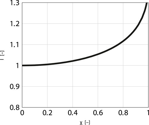
FIGURE 2. Numerical value of I, see Eq. 115, obtained for several values of $\chi =\left[\frac{\mathrm{\Delta }k(1+{\nu }_0)}{3k_0(1-{\nu }_0)}\right]$.

${\left({\mathbb{M}}^{-1}\right)}_{\mathrm{iiii}}=\frac{2}{3}+I\left(\chi \right).(117)$

The next components to be considered are $M_{\mathit{iijj}}^{-1}$, with i ≠ j. They read, from Eq. 87 and Eq. 115, as

${\left({\mathbb{M}}^{-1}\right)}_{\mathrm{iijj}}=-\frac{1}{3}+I\left(\chi \right),\forall i\ne j.(118)$

The shear components read as

${\left({\mathbb{M}}^{-1}\right)}_{\mathrm{ijij}}=1,\forall i\ne j,(119)$

and

${\left({\mathbb{M}}^{-1}\right)}_{\mathrm{ijk\ell }}=0,\forall i\ne j,i\ne k.(120)$

Thus, the auxiliary-to-RVE tensor reads as

$\mathbb{M}=\frac{1}{3I}\left(\begin{array}{cccccc}\hfill 1/3+2I\hfill & \hfill 1/3-I\hfill & \hfill 1/3-I\hfill & \hfill 0\hfill & \hfill 0\hfill & \hfill 0\hfill \\ \hfill 1/3-I\hfill & \hfill 1/3+2I\hfill & \hfill 1/3-I\hfill & \hfill 0\hfill & \hfill 0\hfill & \hfill 0\hfill \\ \hfill 1/3-I\hfill & \hfill 1/3-I\hfill & \hfill 1/3+2I\hfill & \hfill 0\hfill & \hfill 0\hfill & \hfill 0\hfill \\ \hfill 0\hfill & \hfill 0\hfill & \hfill 0\hfill & \hfill 3I\hfill & \hfill 0\hfill & \hfill 0\hfill \\ \hfill 0\hfill & \hfill 0\hfill & \hfill 0\hfill & \hfill 0\hfill & \hfill 3I\hfill & \hfill 0\hfill \\ \hfill 0\hfill & \hfill 0\hfill & \hfill 0\hfill & \hfill 0\hfill & \hfill 0\hfill & \hfill 3I\hfill \end{array}\right).(121)$

Lastly, the real strain concentration tensor field is computed according to Eq. 14 as

$\mathbb{A}\left(\underline{x}\right)=\left(\begin{array}{cccccc}\hfill A_{\mathit{iiii}}\hfill & \hfill A_{\mathit{iijj}}\hfill & \hfill A_{\mathit{iijj}}\hfill & \hfill 0\hfill & \hfill 0\hfill & \hfill 0\hfill \\ \hfill A_{\mathit{iijj}}\hfill & \hfill A_{\mathit{iiii}}\hfill & \hfill A_{\mathit{iijj}}\hfill & \hfill 0\hfill & \hfill 0\hfill & \hfill 0\hfill \\ \hfill A_{\mathit{iijj}}\hfill & \hfill A_{\mathit{iijj}}\hfill & \hfill A_{\mathit{iiii}}\hfill & \hfill 0\hfill & \hfill 0\hfill & \hfill 0\hfill \\ \hfill 0\hfill & \hfill 0\hfill & \hfill 0\hfill & \hfill 1\hfill & \hfill 0\hfill & \hfill 0\hfill \\ \hfill 0\hfill & \hfill 0\hfill & \hfill 0\hfill & \hfill 0\hfill & \hfill 1\hfill & \hfill 0\hfill \\ \hfill 0\hfill & \hfill 0\hfill & \hfill 0\hfill & \hfill 0\hfill & \hfill 0\hfill & \hfill 1\hfill \end{array}\right),(122)$

where

$A_{\mathit{iiii}}\left(\underline{x}\right)=\frac{2}{3}+\frac{1}{3I\left(\chi \right)}\left[\frac{1}{1+\frac{\mathrm{\Delta }k\left(1+{\nu }_0\right)}{3k_0\left(1-{\nu }_0\right)}\text{sin}\left(\frac{2\pi }{{\lambda }_1}{x}_1\right)\text{sin}\left(\frac{2\pi }{{\lambda }_2}{x}_2\right)\text{sin}\left(\frac{2\pi }{{\lambda }_3}{x}_3\right)}\right],(123)$

$A_{\mathit{iijj}}\left(\underline{x}\right)=-\frac{1}{3}+\frac{1}{3I\left(\chi \right)}\left[\frac{1}{1+\frac{\mathrm{\Delta }k\left(1+{\nu }_0\right)}{3k_0\left(1-{\nu }_0\right)}\text{sin}\left(\frac{2\pi }{{\lambda }_1}{x}_1\right)\text{sin}\left(\frac{2\pi }{{\lambda }_2}{x}_2\right)\text{sin}\left(\frac{2\pi }{{\lambda }_3}{x}_3\right)}\right],(124)$

see Eq. 115 and Figure 2 for I(χ).

5.5 Homogenized stiffness of sinusoidally fluctuating microstructure

From Eq. 16, the difference between the homogenized stiffness and the background stiffness ${\mathbb{C}}^0$ reads as

$\mathrm{\Delta }{\mathbb{C}}^{\mathrm{hom}}={\mathbb{C}}^{\mathrm{hom}}-{\mathbb{C}}^0=\left[\frac{1}{V_{\text{RVE}}}\underset{V_{\text{RVE}}}{\int }\left[\mathbb{c}\left(\underline{x}\right)-{\mathbb{C}}^0\right]:\mathbb{A}\left(\underline{x}\right)\mathrm{d}V\left(\underline{x}\right)\right].(125)$

One more time, the components of this tensor will be obtained individually. The only non-vanishing components ΔC_hom,ijkℓ are those with i = j and k = ℓ, due to Eq. 122 and

$\left[c_{\mathit{ijk\ell }}\left(\underline{x}\right)-C_{\mathit{ijk\ell }}^0\right]=\mathrm{\Delta }k\text{sin}\left(\frac{2\pi }{{\lambda }_1}{x}_1\right)\text{sin}\left(\frac{2\pi }{{\lambda }_2}{x}_2\right)\text{sin}\left(\frac{2\pi }{{\lambda }_3}{x}_3\right){\delta }_{ij}{\delta }_{k\ell }.(126)$

Therefore, the components ΔC_hom,iikk read as

$\begin{array}{ll}\hfill \mathrm{\Delta }{C}_{\mathrm{hom},iikk}& =\frac{1}{V_{\text{RVE}}}\underset{V_{\text{RVE}}}{\int }\mathrm{\Delta }k\text{sin}\left(\frac{2\pi }{{\lambda }_1}{x}_1\right)\text{sin}\left(\frac{2\pi }{{\lambda }_2}{x}_2\right)\hfill \\ \hfill & \times \text{sin}\left(\frac{2\pi }{{\lambda }_3}{x}_3\right)\left[\sum _{p=1}^3{A}_{\mathit{ppkk}}\left(\underline{x}\right)\right]\mathrm{d}V\left(\underline{x}\right).\hfill \end{array}(127)$

Thus, inserting Eq. 123 and Eq. 124 into Eq. 127 and applying ${\underline{x}}^{\prime }=\frac{2\pi }{\lambda }\underline{x}$ yields

$\begin{array}{ll}\hfill \mathrm{\Delta }{C}_{\mathrm{hom},iikk}& =\frac{\mathrm{\Delta }k}{I{\left(2\pi \right)}^3}\underset{V_{\text{RVE}}^{\prime }}{\int }\hfill \\ \hfill & \frac{\text{sin}\left(x_1^{\prime }\right)\text{sin}\left(x_2^{\prime }\right)\text{sin}\left(x_3^{\prime }\right)}{1+\frac{\mathrm{\Delta }k\left(1+{\nu }_0\right)}{3k_0\left(1-{\nu }_0\right)}\text{sin}\left(x_1^{\prime }\right)\text{sin}\left(x_2^{\prime }\right)\text{sin}\left(x_3^{\prime }\right)}\mathrm{d}V\left({\underline{x}}^{\prime }\right).\hfill \end{array}(128)$

Integrating Eq. 128 with respect to $x_1^{\prime }$ from −π to π yields

$\begin{array}{ll}\hfill \mathrm{\Delta }{C}_{\mathrm{hom},iik\ell }& =\frac{3k_0\left(1-{\nu }_0\right)}{I\left(1+{\nu }_0\right){\left(2\pi \right)}^2}\left[\underset{-\pi }{\overset{\pi }{\int }}\underset{-\pi }{\overset{\pi }{\int }}\mathrm{d}{x}_2^{\prime }\mathrm{d}{x}_3^{\prime }\right.\hfill \\ \hfill & \left.-\underset{-\pi }{\overset{\pi }{\int }}\underset{-\pi }{\overset{\pi }{\int }}\frac{1}{\sqrt{1-{\psi }^2\left(x_2^{\prime },x_3^{\prime }\right)}}\mathrm{d}{x}_2^{\prime }\mathrm{d}{x}_3^{\prime }\right]\hfill \\ \hfill & =-\frac{3k_0\left(1-{\nu }_0\right)}{\left(1+{\nu }_0\right)}\left[\frac{I\left(\chi \right)-1}{I\left(\chi \right)}\right],\hfill \end{array}(129)$

whereby we have made use of Eq. 114. Clearly, for the stiffness field of Eq. 50, the remaining components vanish, considering Eq. 122 and Eq. 126.

6 Discussion

It is worthwhile to discuss key characteristics of the convolution integral-type mathematical relations for the concentration tensor fields introduced in the present paper. We start by mentioning that Eq. 48 is, to our best knowledge, the first-ever explicit integral formulation for the concentration tensor fields arising from a general microstiffness field. Actually, in the pertinent literature, see, e.g., the review of Zaoui (2002), the mathematical existence of such a field is mentioned, while any corresponding explicit expression is missing.

Our new expression, Eq. 48, provides a common basis for the treatment for virtually any type of microstructure, be they general harmonic microstructures, with microelasticity distributions which can be represented by means of Fourier series, as described in Section 6.5, or even distributions with discontinuities, allowing for the consideration of classical composite material morphologies, arising from the assembly of a finite number of microstructural domains with uniform stiffnesses, normally referred to as “material phases”. Accordingly, the novel method is also apt for large volume fractions of one of the aforementioned domains, i.e., to the so-called “large concentration composition”.

As it is well known that the Green kernel occurring in the aforementioned integral expressions is singular at the point $\underline{x}=\underline{y}$, the corresponding convolutions need to be carried out with care, and it is therefore interesting to compare the solution strategy based on the Poisson’s equation, as applied throughout Section 5, with the more traditional way of evaluating such integrals, namely, by introducing an infinitesimally small sphere around the singularity, and by transforming the volume integral within that sphere to a surface integral across the sphere’s surface. This will be covered in the first subsection of the present Discussion section.

Alternatively, one may wish a numerical confirmation of our new analytical approach to strain concentration tensor fields, and we provide such a confirmation in terms of FFT-based computational homogenization, in the second subsection of the present Discussion section.

It is also instructive to compare our approach to earlier suggestions for the use of a Fredholm integral equation similar to Eq. 36, often referred to as the Lippmann-Schwinger equation; in particular so concerning the domain over which the convolution integral is evaluated, the type of polarization field considered, and the relation of the Fredholm integral equation to the macroscopic strain associated with the RVE. This is the topic of the third subsection of the present Discussion section.

Finally, we discuss the range of validity of the Fredholm integral Eq. 36, and the practical evaluation of the concentration tensor expressions in the case of microstructures which are more general than that with the sinusoidally fluctuating microscopic bulk moduli covered in Section 5. Corresponding deliberations conclude the present Discussion section.

6.1 Singular convolution integrals–Analytical validation by means of Cauchy principal value

All integral expressions defining concentration tensor fields, such as Eq. 14, Eqs. 41–43, Eq. 51, Eq. 65, and Eq. 70, exhibit singularities at $\underline{x}=\underline{y}$, i.e., at $\underline{x}-\underline{y}=-\underline{z}=0$. In Section 5, we circumvented a direct treatment of this singularity, when evaluating Eq. 70 from the solution of the Poisson’s equation, in combination with an auxiliary function in ${\underline{z}}^{\prime }$. In order to check the relevance of this strategy, we here evaluate the integral in Eq. 70 by an alternative approach, sometimes referred to as the Cauchy principal value analysis. Therefore, the integral in Eq. 70 is split into two portions associated with two integration domains: The first one is a sphere around the singular point (with a variable radius ϵ, eventually tending towards zero), and the second one is the remaining (unbounded) three-dimensional space.

Denoting the small spherical domain as V^ϵ, the integral in Eq. 70 can be recast as, see, e.g., Buryachenko (2007), p. 54,

$\begin{array}{ll}\hfill \underset{V^{ϵ}}{\int }\frac{{\partial }^2}{\partial z_1^2}\left(\frac{1}{|\underline{z}|}\right)f\left(\underline{z}\right)\mathrm{d}V\left(\underline{z}\right)=& \underset{V^{ϵ}}{\int }\frac{{\partial }^2}{\partial z_1^2}\left(\frac{1}{|\underline{z}|}\right)\left[f\left(\underline{z}\right)\right.\left.-f\left(0\right)\right]\mathrm{d}V\left(\underline{z}\right)\hfill \\ \hfill & +\left[\underset{V^{ϵ}}{\int }\frac{{\partial }^2}{\partial z_1^2}\left(\frac{1}{|\underline{z}|}\right)\mathrm{d}V\left(\underline{z}\right)\right]f\left(0\right),\hfill \end{array}(130)$

whereby

$f\left(\underline{z}\right)=\text{cos}\left(\frac{2\pi }{\lambda }{z}_1\right)\text{cos}\left(\frac{2\pi }{\lambda }{z}_2\right)\text{cos}\left(\frac{2\pi }{\lambda }{z}_3\right),(131)$

is fully in line with the developments of Eq. 72 and Eq. 73. As stated before, we are interested in the limit case of ϵ → 0 where

$\underset{ϵ\to 0}{\text{lim}}\underset{V^{ϵ}}{\int }\frac{{\partial }^2}{\partial z_1^2}\left(\frac{1}{|\underline{z}|}\right)\left[f\left(\underline{z}\right)-f\left(0\right)\right]\mathrm{d}V\left(\underline{z}\right)=0,(132)$

so that

$\begin{array}{ll}\hfill & \underset{ϵ\to 0}{\text{lim}}\underset{V^{ϵ}}{\int }\frac{{\partial }^2}{\partial z_1^2}\left(\frac{1}{|\underline{z}|}\right)f\left(\underline{z}\right)\mathrm{d}V\left(\underline{z}\right)\hfill \\ \hfill & =\underset{ϵ\to 0}{\text{lim}}\left[\underset{V^{ϵ}}{\int }\frac{{\partial }^2}{\partial z_1^2}\left(\frac{1}{|\underline{z}|}\right)\mathrm{d}V\left(\underline{z}\right)\right]f\left(0\right)\hfill \\ \hfill & =\underset{ϵ\to 0}{\text{lim}}\left[\underset{S^{ϵ}}{\int }\frac{\partial }{\partial z_1}\left(\frac{1}{|\underline{z}|}\right)n_1\mathrm{d}S\left(\underline{z}\right)\right]f\left(0\right),\hfill \end{array}(133)$

whereby we made use of the divergence theorem, with $\underline{n}$ standing for the outward normal onto the spherical surface. Notably, the surface integral in Eq. 133 does not exhibit any singularity any more, since the radius ϵ, however small it may become, never actually reaches zero, so that the integrand in the last integral of Eq. 133 always stays finite. Let us evaluate the latter in more detail: Realizing that

$ϵ=|\underline{x}-\underline{y}|=|-\underline{z}|=|\underline{z}|={\left(z_1^2+z_2^2+z_3^2\right)}^{1/2},(134)$

the integrand in the surface integral of Eq. 133 can be transformed to

$\frac{\partial }{\partial z_1}\left[{\left(z_1^2+z_2^2+z_3^2\right)}^{-1/2}\right]=-z_1{\left(z_1^2+z_2^2+z_3^2\right)}^{-3/2}=-\frac{z_1}{{ϵ}^3}.(135)$

Then, the surface integral in Eq. 133 is preferably evaluated in spherical coordinates, where.

$z_1=ϵ\text{cos}\varphi \text{sin}\theta ,(136)$

$n_1=\text{cos}\varphi \text{sin}\theta ,(137)$

$\mathrm{d}S={ϵ}^2\text{sin}\theta \mathrm{d}\varphi \mathrm{d}\theta ,(138)$

so that use of Eqs. 135–138 in the surface integral of Eq. 133 yields an expression which becomes independent of ϵ, and hence, of the limiting process. In mathematical detail, we have

$\begin{array}{ll}\hfill & \underset{ϵ\to 0}{\text{lim}}\left[\underset{S^{ϵ}}{\int }\frac{\partial }{\partial z_1}\left(\frac{1}{|\underline{z}|}\right)n_1\mathrm{d}S\left(\underline{z}\right)\right]f\left(0\right)\hfill \\ \hfill & =\left[-\underset{\theta =0}{\overset{\pi }{\int }}{\text{sin}}^3\theta \mathrm{d}\theta \underset{\varphi =0}{\overset{2\pi }{\int }}{\text{cos}}^2\varphi \mathrm{d}\varphi \right]f\left(0\right)\hfill \\ \hfill & =-\frac{4\pi }{3}f\left(0\right),\hfill \end{array}(139)$

and hence, since f (0) = 1,

$\underset{V^{ϵ}}{\int }\frac{{\partial }^2}{\partial z_1^2}\left(\frac{1}{|\underline{z}|}\right)f\left(\underline{z}\right)\mathrm{d}V\left(\underline{z}\right)=-\frac{4\pi }{3}(140)$

The result of Eq. 140 is fully equivalent with evaluating Eq. 76 for ${\underline{z}}^{\prime }=0$ and inserting the corresponding result into Eq. 71. This proves the solution strategy for singular integrals, as given through Eqs. 71–77. Accordingly, the small spherical integration domain yields the solution of the entire volume integral (spanning also the entire three-dimensional space outside the small spherical domain); hence, the integral of Eq. 65, when evaluated over the three-dimensional space expect for the small sphere enclosing the singularity at the origin $\underline{z}=0$, vanishes. This last statement can also be found in the book of Buryachenko (2007), namely, as the last equation of (3.29) in the aforementioned reference.

The situation is totally different when it comes to the shear-related concentration tensor components according to Eq. 93. There, the Cauchy principal value needs to be multiplied by sin (0) = 0 so that the integration over the small sphere delivers zero, and it is the domain outside the small sphere, which solely contributes to the integral in Eq. 93. A procedure for solving this regular integral was presented, see Eqs. 94–103.

6.2 Strain concentration tensor fields and homogenized stiffness: Numerical confirmation by means of FFT homogenization

In order to gain further confidence into our novel method, we evaluate the analytically defined strain concentration tensor fields of Eq. 123 and Eq. 124 for a particular numerical choice of sinusoidal microelasticity field, see Table 2 for this choice, and then compare this evaluation to suitably chosen microstrain fields computed by means of the classical FFT homogenization methods proposed by Moulinec and Suquet (1994), Moulinec and Suquet (1998), and widely expanded and used thereafter (Lucarini et al., 2021).

TABLE 2

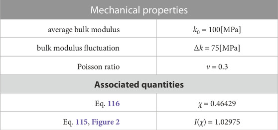
TABLE 2. Mechanical properties and quantities associated to the particular microelastic material, see Eq. 50.

The key idea of FFT homogenization is to start with an estimate for the microstrain fields, to compute a corresponding estimate for the polarization stress field, then test the latter estimate on the Fourier transform of Eq. 33 with $\underline{f}\equiv 0$, reading as

$\widehat{\mathit{\epsilon }}\left(\underline{k}\right)=\delta \left(\underline{k}\right){\mathbf{E}}^0-\widehat{\mathbb{G}}\left(\underline{k}\right):\widehat{\mathit{\tau }}\left(\underline{k}\right),(141)$

with the wave vector $\underline{k}$, and the hat-symbol indicating the Fourier transform, according to

$\widehat{\mathit{\epsilon }}\left(\underline{k}\right)=\frac{1}{{\left(2\pi \right)}^3}{\int }_{{\mathcal{R}}^3}\mathit{\epsilon }\left(\underline{x}\right)\text{exp}\left(-i\underline{k}\cdot \underline{x}\right)\mathrm{d}V\left(\underline{x}\right).(142)$

Namely, prescribing the polarization stress on the right-hand side of Eq. 141 yields a new estimate of microstrain field in the wave domain, which needs to be back-transformed into the traditional location space domain. This new estimate allows for computation of an improved estimate of the polarization stress fields, as described before. The sequential estimation of the polarization stress field (in the location space) and the microstrain field (in the wave space) is repeated until two successive strain estimates differ only very slightly from each other. This algorithm becomes especially appealing if both the Fourier transform and the inverse Fourier transform are realized discretely, on a finite number of locations given by the voxels making up an image. As such a discrete transform can be set up to deliver results in a particularly fast fashion, it is called Fast Fourier transformation, abbreviated as FFT (Cochran et al., 1967), and accordingly, the aforementioned algorithm is referred to as FFT homogenization.

In order to get access to the strain concentration tensor field (which is not the standard target of an FFT homogenization study), we identify the component A_iiii, with i = 1, 2, 3, as the microstrain field component ɛ_ii, with i = 1, 2, 3, which arises from a macroscopic strain tensor of the format $\mathbf{E}={\underline{e}}_i\otimes {\underline{e}}_i$, with ${\underline{e}}_i$ denoting the base vector pointing into the ith direction of an orthonormal base frame. In other words, the only non-vanishing component of the aforementioned macroscopic strain tensor is E_ii = 1. Analogously, component A_iijj, with i, j = 1, 2, 3 and i ≠ j, is the microstrain field component ɛ_ii, with i = 1, 2, 3, arising from a macroscopic strain tensor of the format $\mathbf{E}={\underline{e}}_j\otimes {\underline{e}}_j$.

Different, increasingly fine, FFT discretizations of the investigated sinusoidal microelasticity distribution deliver strain tensor concentration fields which very satisfactorily converge to the analytical solution of Eq. 123 and Eq. 124, see Figure 3 and Figure 4. Accordingly, the FFT-determined homogenized stiffness properties agree virtually perfectly with the analytical results according to Eq. 129, see Table 3. At the same time, our new analytical solution strategy is remarkably efficient from the viewpoint of CPU time: on a Core i5-1035G1 processor in a Lenovo Ideapad S340-15IIL computer, the numerical evaluation of the integral I(χ) according to Eq. 115, the only operation needing non-negligible computer time, lasts for only 0.004 s, while FFT solution processes for 100³ voxels last by a factor of over 6,500 longer, namely, for 26.7 s.

FIGURE 3

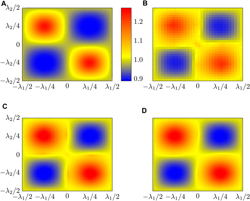
FIGURE 3. Strain concentration field $A_{\mathit{iiii}}(\underline{x})$, i = 1, 2, 3, arising from the sinusoidal microelasticity distribution of Eq. 50, at the plane x_i = λ_i/4, i = 1, 2, 3, obtained (A) analytically from Eq. 123, and numerically by means of FFT (Lucarini et al., 2021) with (B) 32³ voxels, (C) 52³ voxels, and (D) 100³ voxels.

FIGURE 4

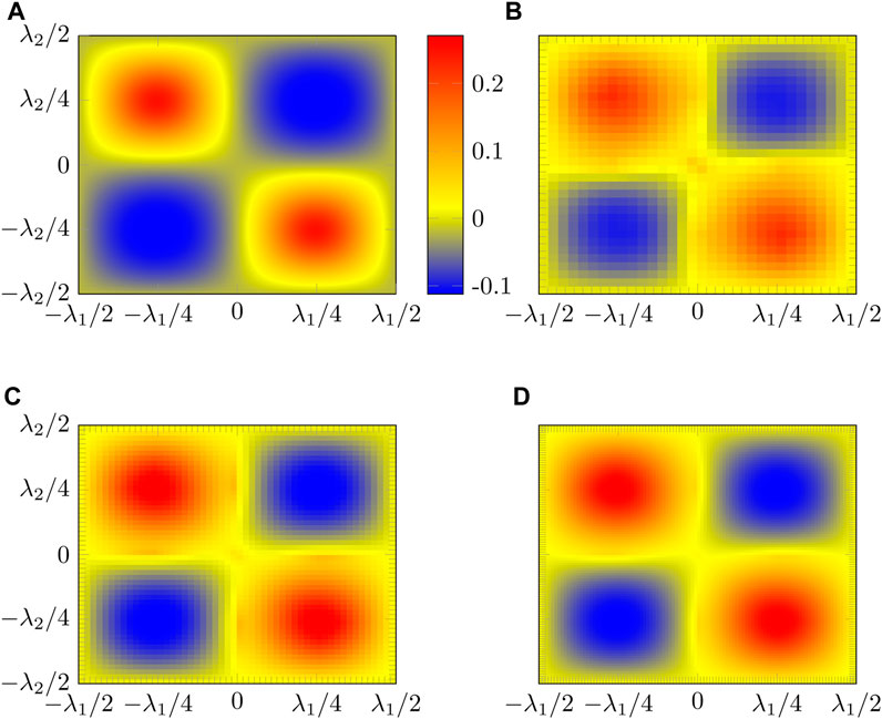
FIGURE 4. Strain concentration field $A_{\mathit{iijj}}(\underline{x})$, i, j, = 1, 2, 3, at the plane x_i = λ_i/4, i, j, = 1, 2, 3, obtained (A) analytically from Eq. 124, and numerically by means of FFT (Lucarini et al., 2021) with (B) 32³ voxels, (C) 52³ voxels, and (D) 100³ voxels.

TABLE 3

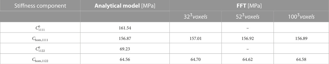
TABLE 3. Numerical value of stiffness tensor components of the benchmark example calculated by means of the proposed analytical model, see Eq. 129, and by FFT with different discretizations.

6.3 Use of the Lippmann-Schwinger equation: Auxiliary problems, integration domains, and macroscopic strains associated with the RVE

From a terminological viewpoint, we note that equations of the format of Eq. 36, irrespective of the chosen integration domains or the format of the polarization stresses, are often referred to as the Lippmann-Schwinger equation, as a similar equation has been proposed by Lippmann and Schwinger (1950) in the field of quantum mechanics. In this context, it is interesting to compare our present contribution to earlier micromechanical applications of the Lippmann-Schwinger equation. A form which is virtually identical to Eq. 36 appears as Eq. 9 in (Molinari and El Mouden, 1996); except for a sign change stemming from the definition of the fourth-order Green operator as the twofold gradient with respect to $\underline{x}$ – this differs from our definition (35). Mathematically speaking, the aforementioned sign change is due to

${\text{grad}}_x{\text{grad}}_x\mathbf{G}\left(\underline{x}-\underline{y}\right)=-{\text{grad}}_x^S{\text{grad}}_y\mathbf{G}\left(\underline{x}-\underline{y}\right).(143)$

However, the actual use of Eq. 9 in (Molinari and El Mouden, 1996) is quite different from our present use of Eq. 36, as Molinari and El Mouden (1996) introduce an infinite number of uniform subfields of microscopic stiffnesses, representing strongly interacting “elastic inclusions” within an RVE of a composite material. At the same time, as a certain commonality of the approach of Molinari and El Mouden (1996) and our present contribution, we note that the latter authors’ strain ɛ⁰ plays exactly the role of our auxiliary strain E⁰: it is the strain applied to the auxiliary homogeneous, infinite matrix which undergoes polarization stresses. However, different from our approach to solve this auxiliary problem so as to provide the microscopic strains as a function of the auxiliary strains, Molinari and El Mouden (1996) apply the strain average rule directly to the Fredholm integral equation, i.e., to their Eq. 9, and this leads to their Eq. 16 linking auxiliary and RVE-related strains. On this basis, they then discuss explicit solutions for finite numbers of inclusions within a periodically repeating cubic cell. In this context, Molinari and El Mouden (1996) apply the strain average rule to an infinite domain, as can be seen from their Eq. 15, while our Eq. 12 is clearly related to the (finite) RVE, and hence to the average rule of Eq. 2, which arises from the Hashin displacement boundary conditions imposed onto the RVE according to Eq. 1. We also note that neither Eq. 9 nor Eq. 16 in (Molinari and El Mouden, 1996) give access to the concentration tensor fields - so that our expression according to Eq. 14, together with Eqs. 41–43, turn out as an interesting original aspect of the present paper.

Eq. 36 of the present paper is also reminiscent of Eq. 2.28 in (Torquato, 1997). However, different from our approach, Torquato (1997) restricts a non-vanishing polarization field to a finite domain within his infinitely large auxiliary problem subjected to some auxiliary strain ɛ⁰, the role of which is comparable to our auxiliary strain E⁰. In this context, he notes that the result of the corresponding convolution integral depends on the shape of the aforementioned finite domain, a situation which does not occur in our anaylsis in which the convolution integrals are evaluated throughout the unbounded auxiliary matrix. Eventually, Torquato (1997) lets his finite polarization domain coincide with the RVE of an anisotropic two-phase composite, for which he identifies stiffness series expansions in powers of “elastic polarizabilities”.

A further difference appears between Eq. 36 of the present contribution and the formally similar Eq. 4 of the famous paper of Moulinec and Suquet (1994), see also (Moulinec and Suquet, 1998). The latter authors introduce the convolution integral directly on the (finite) RVE, noting that a corresponding explicit Green’s function can only be given in the case of periodic displacement boundary conditions imposed onto the RVE, and of corresponding microscopic strains which fluctuate periodically around their average (i.e., around the macroscopic strain). Namely, it is under this periodicity condition, that an explicit solution for the convolution problem exists in the Fourier space, which, in turn, allows for the development of a very efficient algorithm for the mechanical treatment of images made up of pixels or voxels, with the polarization stress being constant throughout one pixel or voxel, respectively.

Green’s operators in convolution integrals over a finite volume (i.e., differing from our present integration over an infinite auxiliary domain) have been already introduced in the 1970s: In this context, Zeller and Dederichs (1973) noted that the corresponding Green’s functions read as $\mathbf{G}(\underline{x},\underline{y})=\mathbf{G}(\underline{y},\underline{x})$, rather than $\mathbf{G}(\underline{x}-\underline{y})=\mathbf{G}(\underline{y}-\underline{x})$, an aspect which was somewhat overlooked by Korringa (1973). However, explicit expressions for the aforementioned Green’s functions are not available, so that Zeller and Dederichs (1973) restricted their analysis to series expansions for small stiffness fluctations, while Kröner (1977) uses convolution integrals over finite volumes for the derivation of bounds for the effective elastic moduli of disordered materials.

Our iterative scheme for solving the Fredholm integral Eq. 36 also bears some similarities with earlier contributions in the field: Kröner (1977) presents an iterative solution for the Lippmann-Schwinger equation formulated directly on the RVE, and Torquato (1997) proposes an iterative scheme which finally delivers the polarization stress as a function of the homogeneous auxiliary strain ɛ⁰.

6.4 Range of validity of Lippmann-Schwinger equation

The practical relevance of the case where the polarization stresses in Eq. 33 outweigh the effect of the microscopic volume forces, which is the prerequisite for the Lippmann-Schwinger Eq. 36 to hold, deserves further discussion: Within the RVE, the microscopic stresses σ fluctuate around their spatial average, which is the macroscopic stress Σ, and the characteristic length scale d of this fluctuation is scale-separated from the length of the RVE, ℓ_RVE, which reads mathematically as

$\frac{\partial \left(\mathit{\sigma }-\mathbf{\Sigma }\right)}{\partial \underline{x}}=\frac{\partial \mathit{\sigma }}{\partial \underline{x}},\mathrm{w}\mathrm{i}\mathrm{t}\mathrm{h}\frac{\Vert \mathit{\sigma }\Vert }{\Vert \frac{\partial \mathit{\sigma }}{\partial \underline{x}}\Vert }=d.(144)$

Due to the mathematical structure of the microscopic equilibrium conditions, see Eq. 5, any microscopic volume forces leading to microscopic stress fluctuations are required to change their sign, i.e., their direction, over distances as small as d. Practically speaking, this is an exceptional case: Even in composites with high contrast in mass density, the corresponding gravitational forces of varying magnitude would always share the same direction; or in other words, practically relevant force fields are often parallel within the RVE. We note in passing, that such micro-parallel force field, directly implying the validity of Eq. 36, even fulfill a force field average rule (Jiménez Segura et al., 2022).

6.5 Practical note concerning generally harmonic microstiffness fluctuations

Finally, we discuss which aspects of Section 5 hold beyond the restriction to sinusoidally fluctuating microstiffnesses, and how the semi-analytical solutions presented in this section may be generalized to generally harmonic microstiffness fluctuations. In this context, the key generalization step would be the representation of any, arbitrarily general continuous microstiffness distribution across a finite RVE by a three-dimensional Fourier series. Generalizing, in this way, the example distribution of Eq. 50 to an arbitrarily inhomogenous bulk modulus distribution Δk (x₁, x₂, x₃) yields

$\mathbb{c}\left(\underline{x}\right)={\mathbb{C}}^0+3\sum _k^{\infty }\sum _l^{\infty }\sum _m^{\infty }{c}_{\mathit{klm}}\text{exp}\left(2\pi i\left[\frac{k{x}_1}{{\lambda }_1}+\frac{l{x}_2}{{\lambda }_2}+\frac{m{x}_3}{{\lambda }_3}\right]\right),(145)$

with i now standing for the imaginary unit, and with the Fourier coefficients c_klm being obtained from

$\begin{array}{ll}\hfill c_{\mathit{klm}}& =\underset{-a}{\overset{a}{\int }}\underset{-a}{\overset{a}{\int }}\underset{-a}{\overset{a}{\int }}\text{exp}\left(-2\pi i\left[\frac{k{x}_1}{{\lambda }_1}+\frac{l{x}_2}{{\lambda }_2}+\frac{m{x}_3}{{\lambda }_3}\right]\right)\hfill \\ \hfill & \times \mathrm{\Delta }k\left(x_1,x_2,x_3\right)\mathrm{d}{x}_1\mathrm{d}{x}_2\mathrm{d}{x}_3.\hfill \end{array}(146)$

In other words, sums of products of any three trigonometric functions, be they sine or cosine,—rather than the product of three sine or three cosine terms—would occur throughout the convolution integrals. However, the effect on the corresponding modifications of Eq. 66 and Eq. 93 are only minor: Thanks to Eq. 67 and

$\text{cos}\left(a+b\right)=\text{cos}\left(a\right)\text{cos}\left(b\right)-\text{sin}\left(a\right)\text{sin}\left(b\right),(147)$

the structure of the integrals in Eq. 70 and Eq. 96 stays unaffected. This shows the considerable potential of our method for material investigation based on Fourier-representation of images (Chung et al., 2007)—as an interesting complement to the popular voxel-based FFT schemes.

7 Conclusion

In the present paper, it is for the first time that explicit integral expressions for the concentration tensor fields arising from generally non-uniform microelasticity distributions have been given. More precisely, the effects of elastic behavior at the microscale are represented by means of the Green’s function formalism, leading to Fredholm integral equations which provide novel, series-type integral expressions for the concentration tensor field. The latter may be analytically solved in cases where the involved integral expressions can be formulated as derivatives of the solutions of the Poisson equation, then providing an unprecedented direct access to macro-to-micro scale transition relations, as expressed by the concentration tensor expressions of Eq. 47, and Eqs. 122–124. This opens new avenues for exploring the mechanical effect of eigenstrains in hierarchical material systems with complex morphologies, as an interesting alternative to classical computational homogenization. The new approach also provides semi-analytical access to the homogenized stiffness, such as that calculated for a microstructure with sinusoidally fluctuating bulk moduli, see Eq. 16 and Eq. 129. Since I(χ) ≥ 1, see Figure 2, the resulting homogenized stiffness, ${\mathbb{C}}^{\mathrm{hom}}$, is smaller than or equal to the average stiffness, ${\mathbb{C}}^0$. This is fully consistent with the famous result of Voigt (1889) that the average over the microstiffness is larger than the homogenized stiffness, in the sense that (Zaoui, 2002)

$\mathbf{E}:\left(⟨{\mathbb{A}}^T:\mathbb{c}:\mathbb{A}⟩-{\mathbb{C}}^{\mathrm{hom}}\right):\mathbf{E}\ge 0,\forall \mathbf{E}.(148)$

Besides its obvious fundamental knowledge-related and conceptual merits, the new methods appears as extremely advantegeous from a computational viewpoint, in particular if the microstructure can be represented by just a few elements of the series given in Section 6.5, because relevant computational power is needed only for the one-time determination of the Fourier coefficients and the value of the integral occurring in the function graphed in Figure 2; whereby the latter my be even represented by some suitably chosen fitting function.

Nevertheless, as regards classical composite microstructures, well-known homogenization methods based on the Eshelby-Laws matrix-inhomogeneity problem, such as suitable generalizations of the Mori-Tanaka method (Benveniste, 1987), accounting for symmetrization strategies if required (Sevostianov and Kachanov, 2014; Jiménez Segura et al., 2023), may turn out as more efficient than an approach starting from the general expression given in Eq. 48 and Eq. 49. This underlines the sustained success of advanced composite mechanics in the classical sense.

Data availability statement

The original contributions presented in the study are included in the article/Supplementary Material, further inquiries can be directed to the corresponding author.

Author contributions

NJ: investigation, methodology, formal analysis, computation, visualization, writing—original draft, review and editing. BP: supervision, conceptualization, funding acquisition, methodology, formal analysis, writing—original draft, writing—review and editing. CH: supervision, conceptualization, funding acquisition, methodology, formal analysis, writing—review and editing.

Funding

The authors gratefully acknowledge financial support in the framework of the European Union’s Horizon 2020 research and innovation programme under the Marie Skłodowska-Curie grant agreement No. 764691. The authors acknowledge TU Wien Bibliothek for financial support through its Open Access Funding Programme.

Conflict of interest

The authors declare that the research was conducted in the absence of any commercial or financial relationships that could be construed as a potential conflict of interest.

Publisher’s note

All claims expressed in this article are solely those of the authors and do not necessarily represent those of their affiliated organizations, or those of the publisher, the editors and the reviewers. Any product that may be evaluated in this article, or claim that may be made by its manufacturer, is not guaranteed or endorsed by the publisher.

References

Benveniste, Y. (1987). A new approach to the application of Mori-Tanaka’s theory in composite materials. Mech. Mater. 6, 147–157. doi:10.1016/0167-6636(87)90005-6

CrossRef Full Text | Google Scholar

Benveniste, Y., Dvorak, G. J., and Chen, T. (1991). On diagonal and elastic symmetry of the approximate effective stiffness tensor of heterogeneous media. J. Mech. Phys. Solids 39, 927–946. doi:10.1016/0022-5096(91)90012-d

CrossRef Full Text | Google Scholar

Bernard, O., Ulm, F.-J., and Lemarchand, E. (2003). A multiscale micromechanics-hydration model for the early-age elastic properties of cement-based materials. Cem. Concr. Res. 33, 1293–1309. doi:10.1016/s0008-8846(03)00039-5

CrossRef Full Text | Google Scholar

Bertrand, E., and Hellmich, C. (2009). Multiscale elasticity of tissue engineering scaffolds with tissue-engineered bone: A continuum micromechanics approach. J. Eng. Mech. 135, 395–412. doi:10.1061/(asce)0733-9399(2009)135:5(395)

CrossRef Full Text | Google Scholar

Brisard, S., and Dormieux, L. (2010). FFT-based methods for the mechanics of composites: A general variational framework. Comput. Mater. Sci. 49, 663–671. doi:10.1016/j.commatsci.2010.06.009

CrossRef Full Text | Google Scholar

Buchner, T., Königsberger, M., Jäger, A., and Füssl, J. (2022). A validated multiscale model linking microstructural features of fired clay brick to its macroscopic multiaxial strength. Mech. Mater. 170, 104334. doi:10.1016/j.mechmat.2022.104334

CrossRef Full Text | Google Scholar

Buryachenko, V. (2007). Micromechanics of heterogeneous materials. Springer Science and Business Media.

Google Scholar

Cai, X., Brenner, R., Peralta, L., Olivier, C., Gouttenoire, P.-J., Chappard, C., et al. (2019). Homogenization of cortical bone reveals that the organization and shape of pores marginally affect elasticity. J. R. Soc. Interface 16, 20180911. doi:10.1098/rsif.2018.0911

PubMed Abstract | CrossRef Full Text | Google Scholar

Chung, M. K., Dalton, K. M., Shen, L., Evans, A. C., and Davidson, R. J. (2007). Weighted Fourier series representation and its application to quantifying the amount of gray matter. IEEE Trans. Med. Imaging 26, 566–581. doi:10.1109/tmi.2007.892519

PubMed Abstract | CrossRef Full Text | Google Scholar

Cochran, W., Cooley, J., Favin, D., Helms, H., Kaenel, R., Lang, W., et al. (1967). What is the fast Fourier transform? Proc. IEEE 55, 1664–1674. doi:10.1109/PROC.1967.5957

CrossRef Full Text | Google Scholar

Dvorak, G. J. (2012). Micromechanics of composite materials. Springer Science and Business Media.

Google Scholar

Eshelby, J. D. (1957). The determination of the elastic field of an ellipsoidal inclusion, and related problems. Proc. R. Soc. Lond. Ser. A Math. Phys. Sci. 241, 376–396.

Google Scholar

Feng, T., Jia, M., Xu, W., Wang, F., Li, P., Wang, X., et al. (2022). Three-dimensional mesoscopic investigation of the compression mechanical properties of ultra-high performance concrete containing coarse aggregates. Cem. Concr. Compos. 133, 104678. doi:10.1016/j.cemconcomp.2022.104678

CrossRef Full Text | Google Scholar

Fredholm, I. (1900). Sur les équations de l’équilibre d’un corps solide élastique. Acta Math. 23, 1–42. doi:10.1007/bf02418668

CrossRef Full Text | Google Scholar

Fritsch, A., Dormieux, L., and Hellmich, C. (2006). Porous polycrystals built up by uniformly and axisymmetrically oriented needles: Homogenization of elastic properties. Comptes Rendus Mécanique 334, 151–157. doi:10.1016/j.crme.2006.01.008

CrossRef Full Text | Google Scholar

Fritsch, A., Dormieux, L., Hellmich, C., and Sanahuja, J. (2009a). Mechanical behavior of hydroxyapatite biomaterials: An experimentally validated micromechanical model for elasticity and strength. J. Biomed. Mater. Res. Part A 88A, 149–161. doi:10.1002/jbm.a.31727

PubMed Abstract | CrossRef Full Text | Google Scholar

Fritsch, A., Hellmich, C., and Dormieux, L. (2009b). Ductile sliding between mineral crystals followed by rupture of collagen crosslinks: Experimentally supported micromechanical explanation of bone strength. J. Theor. Biol. 260, 230–252. doi:10.1016/j.jtbi.2009.05.021

PubMed Abstract | CrossRef Full Text | Google Scholar

Fritsch, A., Hellmich, C., and Young, P. (2013). Micromechanics-derived scaling relations for poroelasticity and strength of brittle porous polycrystals. J. Appl. Mech. 80, 020905. doi:10.1115/1.4007922

CrossRef Full Text | Google Scholar

Fritsch, A., and Hellmich, C. (2007). ‘Universal’ microstructural patterns in cortical and trabecular, extracellular and extravascular bone materials: Micromechanics-based prediction of anisotropic elasticity. J. Theor. Biol. 244, 597–620. doi:10.1016/j.jtbi.2006.09.013

PubMed Abstract | CrossRef Full Text | Google Scholar

Grimal, Q., Raum, K., Gerisch, A., and Laugier, P. (2011). A determination of the minimum sizes of representative volume elements for the prediction of cortical bone elastic properties. Biomechanics Model. Mechanobiol. 10, 925–937. doi:10.1007/s10237-010-0284-9

PubMed Abstract | CrossRef Full Text | Google Scholar

Guo, W., Han, F., Jiang, J., and Xu, W. (2022). A micromechanical framework for thermo-elastic properties of multiphase cementitious composites with different saturation. Int. J. Mech. Sci. 224, 107313. doi:10.1016/j.ijmecsci.2022.107313

CrossRef Full Text | Google Scholar

Hashin, Z. (1983). Analysis of composite materials—a survey. J. Appl. Mech. 50, 481–505. doi:10.1115/1.3167081

CrossRef Full Text | Google Scholar

Hashin, Z. (1963). Theory of mechanical behavior of heterogeneous media. Philidelphia, Pa: Towne School of Civil and Mechanical Engineering, University of Pennsylvania.

Google Scholar

Hashin, Z. (1965). Viscoelastic behavior of heterogeneous media. J. Appl. Mech. 32, 630–636. doi:10.1115/1.3627270

CrossRef Full Text | Google Scholar

Hellmich, C., Barthélémy, J.-F., and Dormieux, L. (2004). Mineral–collagen interactions in elasticity of bone ultrastructure – A continuum micromechanics approach. Eur. J. Mech. - A/Solids 23, 783–810. doi:10.1016/j.euromechsol.2004.05.004

CrossRef Full Text | Google Scholar

Hellmich, C., and Mang, H. (2005). Shotcrete elasticity revisited in the framework of continuum micromechanics: From submicron to meter level. J. Mater. Civ. Eng. 17, 246–256. doi:10.1061/(asce)0899-1561(2005)17:3(246)

CrossRef Full Text | Google Scholar

Hervé, E., and Zaoui, A. (1993). inclusion-based micromechanical modelling. Int. J. Eng. Sci. 31, 1–10. doi:10.1016/0020-7225(93)90059-4

CrossRef Full Text | Google Scholar

Hill, R. (1963). Elastic properties of reinforced solids: Some theoretical principles. J. Mech. Phys. Solids 11, 357–372. doi:10.1016/0022-5096(63)90036-x

CrossRef Full Text | Google Scholar

Hofstetter, K., Hellmich, C., and Eberhardsteiner, J. (2005). Development and experimental validation of a continuum micromechanics model for the elasticity of wood. Eur. J. Mech. - A/Solids 24, 1030–1053. doi:10.1016/j.euromechsol.2005.05.006

CrossRef Full Text | Google Scholar

Horwitz, A. (2001). A version of Simpson’s rule for multiple integrals. J. Comput. Appl. Math. 134, 1–11. doi:10.1016/s0377-0427(00)00444-1

CrossRef Full Text | Google Scholar

Jiménez Segura, N., Pichler, B. L., and Hellmich, C. (2023). Concentration tensors preserving elastic symmetry of multiphase composites. Mech. Mater. 178, 104555. doi:10.1016/j.mechmat.2023.104555

CrossRef Full Text | Google Scholar

Jiménez Segura, N., Pichler, B. L., and Hellmich, C. (2022). Stress average rule derived through the principle of virtual power. ZAMM - J. Appl. Math. Mech./Zeitschrift für Angewandte Math. und Mech. 102, e202200091. doi:10.1002/zamm.202200091

CrossRef Full Text | Google Scholar

Kneer, G. (1965). Über die Berechnung der Elastizitätsmoduln vielkristalliner Aggregate mit Textur. Phys. Status Solidi (b) 9, 825–838. doi:10.1002/pssb.19650090319

CrossRef Full Text | Google Scholar

Königsberger, M., Hlobil, M., Delsaute, B., Staquet, S., Hellmich, C., and Pichler, B. (2018). Hydrate failure in itz governs concrete strength: A micro-to-macro validated engineering mechanics model. Cem. Concr. Res. 103, 77–94. doi:10.1016/j.cemconres.2017.10.002

CrossRef Full Text | Google Scholar

Korringa, J. (1973). Theory of elastic constants of heterogeneous media. J. Math. Phys. 14, 509–513. doi:10.1063/1.1666346

CrossRef Full Text | Google Scholar

Kröner, E. (1958). Berechnung der elastischen Konstanten des Vielkristalls aus den Konstanten des Einkristalls [Calculation of the elastic constant of the multi-crystal from the constants of the single crystals]. Z. für Phys. 151, 504–518.

Google Scholar

Kröner, E. (1977). Bounds for effective elastic moduli of disordered materials. J. Mech. Phys. Solids 25, 137–155. doi:10.1016/0022-5096(77)90009-6

CrossRef Full Text | Google Scholar

Levin, V. M. (1967). Thermal expansion coefficient of heterogeneous materials. Mekhanika Tverd. Tela 2, 83–94.

Google Scholar

Lipinski, P., Barhdadi, E. H., and Cherkaoui, M. (2006). Micromechanical modelling of an arbitrary ellipsoidal multi-coated inclusion. Philos. Mag. 86, 1305–1326. doi:10.1080/14786430500343868

CrossRef Full Text | Google Scholar

Lippmann, B. A., and Schwinger, J. (1950). Variational principles for scattering processes. I. Phys. Rev. 79, 469–480. doi:10.1103/physrev.79.469

CrossRef Full Text | Google Scholar

Lucarini, S., Upadhyay, M., and Segurado, J. (2021). Fft based approaches in micromechanics: Fundamentals, methods and applications. Model. Simul. Mater. Sci. Eng. 30, 023002. doi:10.1088/1361-651x/ac34e1

CrossRef Full Text | Google Scholar

Moës, N., Cloirec, M., Cartraud, P., and Remacle, J. F. (2003). A computational approach to handle complex microstructure geometries. Comput. Methods Appl. Mech. Eng. 192, 3163–3177. doi:10.1016/s0045-7825(03)00346-3

CrossRef Full Text | Google Scholar

Molinari, A., and El Mouden, M. (1996). The problem of elastic inclusions at finite concentration. Int. J. Solids Struct. 33, 3131–3150. doi:10.1016/0020-7683(95)00275-8

CrossRef Full Text | Google Scholar

Mori, T., and Tanaka, K. (1973). Average stress in matrix and average elastic energy of materials with misfitting inclusions. Acta Metall. 21, 571–574. doi:10.1016/0001-6160(73)90064-3

CrossRef Full Text | Google Scholar

Moulinec, H., and Suquet, P. (1994). A fast numerical method for computing the linear and nonlinear properties of composites. Comptes-Rendus l’Académie Sci. Série II 318, 1417–1423.

Google Scholar

Moulinec, H., and Suquet, P. (1998). A numerical method for computing the overall response of nonlinear composites with complex microstructure. Comput. Methods Appl. Mech. Eng. 157, 69–94. doi:10.1016/s0045-7825(97)00218-1

CrossRef Full Text | Google Scholar

Pahr, D. H., and Zysset, P. K. (2008). Influence of boundary conditions on computed apparent elastic properties of cancellous bone. Biomechanics Model. Mechanobiol. 7, 463–476. doi:10.1007/s10237-007-0109-7

PubMed Abstract | CrossRef Full Text | Google Scholar

Pichler, B., Hellmich, C., Eberhardsteiner, J., Wasserbauer, J., Termkhajornkit, P., Barbarulo, R., et al. (2013). Effect of gel–space ratio and microstructure on strength of hydrating cementitious materials: An engineering micromechanics approach. Cem. Concr. Res. 45, 55–68. doi:10.1016/j.cemconres.2012.10.019

CrossRef Full Text | Google Scholar

Pichler, B., and Hellmich, C. (2011). Upscaling quasi-brittle strength of cement paste and mortar: A multi-scale engineering mechanics model. Cem. Concr. Res. 41, 467–476. doi:10.1016/j.cemconres.2011.01.010

CrossRef Full Text | Google Scholar

Rosen, B. W., and Hashin, Z. (1970). Effective thermal expansion coefficients and specific heats of composite materials. Int. J. Eng. Sci. 8, 157–173. doi:10.1016/0020-7225(70)90066-2

CrossRef Full Text | Google Scholar

Sanahuja, J., Dormieux, L., Meille, S., Hellmich, C., and Fritsch, A. (2010). Micromechanical explanation of elasticity and strength of gypsum: From elongated anisotropic crystals to isotropic porous polycrystals. J. Eng. Mech. 136, 239–253. doi:10.1061/(asce)em.1943-7889.0000072

CrossRef Full Text | Google Scholar

Scheiner, S., Sinibaldi, R., Pichler, B., Komlev, V., Renghini, C., Vitale-Brovarone, C., et al. (2009). Micromechanics of bone tissue-engineering scaffolds, based on resolution error-cleared computer tomography. Biomaterials 30, 2411–2419. doi:10.1016/j.biomaterials.2008.12.048

PubMed Abstract | CrossRef Full Text | Google Scholar

Sevostianov, I., and Kachanov, M. (2014). On some controversial issues in effective field approaches to the problem of the overall elastic properties. Mech. Mater. 69, 93–105. doi:10.1016/j.mechmat.2013.09.010

CrossRef Full Text | Google Scholar

Ting, T. C. T., and Lee, V.-G. (1997). The three-dimensional elastostatic Green’s function for general anisotropic linear elastic solids. Q. J. Mech. Appl. Math. 50, 407–426. doi:10.1093/qjmam/50.3.407

CrossRef Full Text | Google Scholar

Tonon, F., Pan, E., and Amadei, B. (2001). Green’s functions and boundary element method formulation for 3D anisotropic media. Comput. Struct. 79, 469–482. doi:10.1016/s0045-7949(00)00163-2

CrossRef Full Text | Google Scholar

Torquato, S. (1997). Effective stiffness tensor of composite media—I. Exact series expansions. J. Mech. Phys. Solids 45, 1421–1448. doi:10.1016/s0022-5096(97)00019-7

CrossRef Full Text | Google Scholar

Voigt, W. (1889). Über die Beziehung zwischen den beiden Elasticitätsconstanten isotroper Körper [On the relation between the elasticity constants of isotropic bodies]. Ann. Phys. 274, 573–587. doi:10.1002/andp.18892741206

CrossRef Full Text | Google Scholar

Wang, H., Hellmich, C., Yuan, Y., Mang, H., and Pichler, B. (2018). May reversible water uptake/release by hydrates explain the thermal expansion of cement paste? — Arguments from an inverse multiscale analysis. Cem. Concr. Res. 113, 13–26. doi:10.1016/j.cemconres.2018.05.008

CrossRef Full Text | Google Scholar

Whittaker, E., and Robinson, G. (1967). “The trapezoidal and parabolic rules,”in The calculus of observations: A treatise on numerical mathematics (Dover, New York: Cope Press), 156–158.

Google Scholar

Willis, J. R. (1977). Bounds and self-consistent estimates for the overall properties of anisotropic composites. J. Mech. Phys. Solids 25, 185–202. doi:10.1016/0022-5096(77)90022-9

CrossRef Full Text | Google Scholar

Wolfram, U., Peña Fernández, M., McPhee, S., Smith, E., Beck, R. J., Shephard, J. D., et al. (2022). Multiscale mechanical consequences of ocean acidification for cold-water corals. Sci. Rep. 12, 8052. doi:10.1038/s41598-022-11266-w

CrossRef Full Text | Google Scholar

Xie, L., Zhang, C., Sladek, J., and Sladek, V. (2016). Unified analytical expressions of the three-dimensional fundamental solutions and their derivatives for linear elastic anisotropic materials. Proc. R. Soc. A Math. Phys. Eng. Sci. 472, 20150272. doi:10.1098/rspa.2015.0272

PubMed Abstract | CrossRef Full Text | Google Scholar

Xu, W., Wu, F., Jiao, Y., and Liu, M. (2017). A general micromechanical framework of effective moduli for the design of nonspherical nano- and micro-particle reinforced composites with interface properties. Mater. Des. 127, 162–172. doi:10.1016/j.matdes.2017.04.075

CrossRef Full Text | Google Scholar

Xu, W., Wu, Y., and Gou, X. (2019). Effective elastic moduli of nonspherical particle-reinforced composites with inhomogeneous interphase considering graded evolutions of elastic modulus and porosity. Comput. Methods Appl. Mech. Eng. 350, 535–553. doi:10.1016/j.cma.2019.03.021

CrossRef Full Text | Google Scholar

Xu, W., Wu, Y., and Jia, M. (2018). Elastic dependence of particle-reinforced composites on anisotropic particle geometries and reinforced/weak interphase microstructures at nano- and micro-scales. Compos. Struct. 203, 124–131. doi:10.1016/j.compstruct.2018.07.009

CrossRef Full Text | Google Scholar

Zaoui, A. (2002). Continuum micromechanics: Survey. J. Eng. Mech. 128, 808–816. doi:10.1061/(asce)0733-9399(2002)128:8(808)

CrossRef Full Text | Google Scholar

Zeller, R., and Dederichs, P. (1973). Elastic constants of polycrystals. Phys. Status Solidi (b) 55, 831–842. doi:10.1002/pssb.2220550241

CrossRef Full Text | Google Scholar

Zienkiewicz, O. C., Taylor, R. L., and Zhu, J. Z. (2005). The finite element method: Its basis and fundamentals. Elsevier.

Google Scholar