Analysis of unsteady thin film flows over the porous and moving surfaces of variable thickness: Unsteady and non-linear kinematics of sheet

1 Introduction

The global nature of thin film and its technological uses have been identified in many physical and engineering problems. Therefore, the understanding of its mechanics is important in many applications. Most of the industrial systems and the different processes associated with them have been explained through concepts of on thin film flow. The thin film technology is the foundation of amazing development in solid state electronics. Therefore, the scientists worked hard and ascertained the usefulness of the optical properties of metal films, its technical advantages and the human interests associated with the characteristics of two dimensional solid, whereas, it has vast applications in industry and technology of thin films. A typical thin film flow consists of an expanse of metals, partially bounded by a solid or gas or liquid substrate with a (free) surface where the metals such as the liquids are exposed to another fluid (usually a gas and most often air in applications). Stretching/shrinking problem of thin film has one of the most common and stringent applications in industries. On the other hand, shrinking films are widely used for packing of industrial products in factories, whereas, unwanted heat is also produced during this phenomenon and in most cases, it does not affect the flow mechanism during the flow processes. Furthermore, shrinking phenomenon has been frequently used for analyzing the flow in small and narrow pores in order to measure the capillary effects during osmosis processes. The shrinking and swelling properties of agricultural clay soil and boilers are most serious issues, therefore, the most relevant and significant variations in hydraulic and mechanical properties of these soils will eventually disturb the flow, transport and thermodynamics behaviors, whereas, agricultural progresses and environmental improvements are not possible without the perfect simulations of such circumstances. Thin film flow has played significant role in many physical problems of human uses. Most of the engineering systems are composed of heat exchangers, which are commonly used for cooling of machineries, devices and surfaces, as well as it also plays significant role in lubrication processes between small rotating parts, to coat sheets, walls and surfaces and to clean see water by removing oil slicks from it. The formation of tear film in the eyes and mucus linings of the airways and lungs are the uses of thin film flow in biological systems. A thin film is a layer of material ranging from fractions of a nanometer (monolayer) to several micrometers in thickness. Thin films are used for the coating of the household mirror which typically has a thin metal coating on the back of the glass to form a reflective interface.Certainly, we provided concrete investigations of thin film flow over surfaces through which injection and suction can take place, whereas, we came across the evidences where stretching and shrinking flow contribute to such flow. Furthermore, we also emphasized that thin film flow maintained on surfaces of a variable thickness. More specifically, we presented the detailed history and the latest developments in the analysis of thin film flows. Sakiadis (Sakiadis, 1961a; Sakiadis, 1961b) solved a modeled problem of fluid motion maintained over a stretching plate, whereas, the sheet moved with a constant speed. A new model of variable stretching velocity is presented by Crane (Crane, 1970). The classical simulations of Sakiadis (Sakiadis, 1961a; Sakiadis, 1961b) played a key role in the formulation of flow problems over a stretching sheet. However, the work of Sakiadis was generalized and refined by many researchers, whereas, Crane (Crane, 1970) extended the work of Sakiadis for variable stretching velocity and solved the governing non-linear boundary layer equations exactly in the closed form. The remarkable ideas of Crane and Sakiadis have been highly obliged and adopted by researchers for different situations and types of fluids. This section is mainly categorized on the bases of physical flow models, appeared in the literature time to time. They clearly described the fluid motion heat and mass transfer in certain systems. Tremendous improvements have been made in the notable work of Sakiadis and Crane by introducing thermal and mass diffusion characteristics in the previous problems of them, and a special model is developed on the bases of previous studies for thin film flows. Sparrow (Sparrow and Gregg, 1959) treated thin film condensation by using the approach of boundary-layer approximation. He produced remarkable results on the behavior of a thin film over a stretching surface. Wang (1990) investigated unsteady thin film flow on a stretching plate within a boundary layer. Tan et al. (1990) found interesting solutions for the transport of heat in a thin film by assuming a spatially periodic temperature along the plate. Burelbach et al. (1990) verified the work of (Tan et al., 1990) by performing experiments. Dandapat and Ray (1994) presented an accurate model for thermo-capillary process in a thin film flow on a rotating disk. Andersson et al. (1996) explained the idea of a thin film flow on the transient stretching plate for power law fluid. Dandapat et al. (2003) analyzed the diffusion of heat in a thin film flow on the stretching plate moving with time dependent velocity. Dandapat and Maity (2006) studied the unsteady thin film flow over stretching plate and they found the boundary layer type solution and it is confirmed that the two layers (thin film and boundary layer) are exactly matched at certain points. Dandapat et al. (2006) emphasized on the solution for a variable thin film on stretching sheet, whereas, the film thickness is strictly changed with both space and time variables in this case. However, Chen (2006) found the consequences of heat transfer in the flow of a thin film over a transient stretching sheet for power law fluids by considering viscous dissipation term in the modeled equations. Wang (2006) presented analytical solutions to the problem of a thin film, maintained on a transient stretching plate. Andersson et al. (2000) solved the problem of heat diffusion in a thin film flow over a transient stretching plate. Liu and Andersson (2008) presented the generalized concept for the model problem of Andersson et al. (2000) and they studied the diffusion of heat in a thin film, driven by a transient stretching plate. Abbas et al. (2008) modified the approach of Wang (2006) by considering a thin film flow of a non-newtonian second grade fluid on an unsteady stretching surface. Santra and Dandapat (2009) investigated to remove the constraints of planarity and linear stretching for the transport of heat and thermo capillarity. Noor et al. (2010) also extended the modeled problem of Wang (2006) and they found a solution for MHD flows and generalized surface temperature. Mostly recently, flow of different fluids have been discussed over a porous and deforming surfaces in different research articles e.g., see (Ali et al., 2022; Turkyilmazoglu, 2022a; Turkyilmazoglu, 2022b; Krishna et al., 2022; Siddiqui and Turkyilmazoglu, 2022). In these research article the authors have emphasized on the fluid motion, maintained over surfaces of different structure behavior of kinematics of surfaces, types of fluids and mechanism which affects the motion of fluids in advanced setups. All these mechanism have been analyses on flow in these papers very intelligently. In the present work, we have analyzed the new and multiple dimensions of classical problems of thin film flow over a moving and porous sheet of variable thickness. By taken into account the nature and kinds of injection (suction) and moving velocities of the sheet, we categorically emphasized the behavior of thin film flow. Different cases are checked for the non-unifrom kinematics of the sheet of variable size and thin film. All the previous cases of such simulation, already used in the literature, have been recovered easily from the present simulations. The present system of partial differential equations and boundary conditions are transformed into ordinary differential equations on the basis of these new variables, and the final system is solved by bvp4c technique. The classical problems of this film flow have been retrieved from one case for special choice of the parameters values. Furthermore, we obtained the published results of (Wang, 1990; Andersson et al., 2000; Dandapat et al., 2003; Liu and Andersson, 2008) in such situations. Note that the classical simulations of this film flow problem contain two parameters, whereas, we dealt with seven different parameters in of present simulations.

2 Formulation of the problem

The flow of viscous thin film is taken over a porous sheet of variable thickness and the plate is moved in both forward and backward directions with variable velocity, whereas, the injection and suction velocities of the fluid through the porous sheet are non-uniform. Note that we explored different kinds of non-linear forms of five quantities associated with the geometry of sheet, structure of thin film along with the nature of boundary layer and the field variables, defined at the two surfaces in such a way that they exactly transformed the BVP of PDEs into BVP of ODEs. As a result we have obtained a generalized version of thin film flow in such circumstances. We need to evaluate the behavior of thin film within a momentum boundary layer. The constitutive equations, which have governed the flow of viscous thin film and used for the simulation of most complex problem, are the continuity and momentum equations. The boundary layer form of these governing equations is presented here and they are demonstrated in many research articles, e.g., see (Andersson et al., 2000; Dandapat et al., 2003; Liu and Andersson, 2008):

$\frac{\partial u}{\partial x}+\frac{\partial v}{\partial y}=0,(1)$

$\frac{\partial u}{\partial t}+u\frac{\partial u}{\partial x}+v\frac{\partial u}{\partial y}=\nu \frac{{\partial }^{2}u}{\partial y^2}.(2)$

The porous sheet of variable thickness has the abilities to move in its own plane at either direction. The axial and normal velocities are prescribed at the surface of the sheet, so we imposed the following boundary conditions at the variable surface of the sheet and thin film:

$\begin{array}{ll}\hfill u& =U\left(x,t\right),v=V\left(x,t\right),y=f\left(x,t\right),v=w\left(x,t\right)\frac{Dr\left(x,t\right)}{Dt},\frac{\partial u}{\partial y}=0,\hfill \\ \hfill & y=r\left(x,t\right).\hfill \end{array}(3)$

Note that U(x, t) defines the motion of the sheet at its own plane in both forward and backward directions, whereas, V indicates the fluid’s velocity, which enters/leaves through the porous surface of the sheet. On the other hand w(x, t) is controlling parameter for the rate of deformation of the thin film. Similarly f(x, t) represents the variable thickness of sheet and r(x, t) is used for variable size of the thin film. Moreover, $\frac{D}{Dt}$ is the material time derivative and it is defined as $\frac{D}{Dt}=\frac{\partial }{\partial t}+(\mathbf{V}.\nabla )$ where V = (u, v), $\nabla =(\frac{\partial }{\partial x},\frac{\partial }{\partial y})$. Note that u(v) is the velocity component in x(y) direction. Next our aim is to find the similarity transformation for generalized problem presented in Eqs. (1–3). For this reason, we defined the velocity components u, v and the similarity variable (η) in view of the boundaries inputs and independent variables as:

$u=p\left(x,t\right)g\left(\eta \right),v=q\left(x,t\right)h\left(\eta \right),\text{where}\eta =\frac{y-f\left(x,t\right)}{r\left(x,t\right)}(4)$

In the above Eq. 4, g(η) and h(η) are the representatives of the velocity components u and v, respectively. The above similarity variables/transformations are substituted into the governing PDEs in Eqs. 1, 2 then we get the following Eqs. 5, 6. In this system, the coefficients of ODEs are variable and they are depending upon the independent quantities x and t. We have focused on the self similar solutions of the problem and they can be easily achieved if all these variable coefficients in the system of ODE’s should independent of x and t. We tried to avail all such choices and exhaust all options for searching these self similar solutions, therefore, we proceed as:

$h^{\prime }+{\alpha }_{1}g-{\alpha }_2{g}^{\prime }-{\alpha }_3\eta g^{\prime }=0,(5)$

$g^{″}-{\alpha }_{4}h{g}^{\prime }+{\alpha }_5{g}^{\prime }-{\alpha }_{6}g+{\alpha }_7\eta g^{\prime }+{\alpha }_{8}g{g}^{\prime }-{\alpha }_9{g}^2+{\alpha }_{10}\eta g{g}^{\prime }=0.(6)$

The different coefficients in Eqs. 5, 6 have the final form as:

$\begin{array}{cc}\hfill & {\alpha }_1=\frac{r\left(x,t\right)p_x\left(x,t\right)}{q\left(x,t\right)},{\alpha }_2=\frac{p\left(x,t\right)f_x\left(x,t\right)}{q\left(x,t\right)},{\alpha }_3=\frac{p\left(x,t\right)r_x\left(x,t\right)}{q\left(x,t\right)},\hfill \\ \hfill & {\alpha }_4=\frac{q\left(x,t\right)r\left(x,t\right)}{\nu },{\alpha }_5=\frac{r\left(x,t\right)f_t\left(x,t\right)}{\nu },{\alpha }_6=\frac{r^2\left(x,t\right)p_t\left(x,t\right)}{\nu p\left(x,t\right)},\hfill \\ \hfill & {\alpha }_7=\frac{r\left(x,t\right)r_t\left(x,t\right)}{\nu },{\alpha }_8=\frac{p\left(x,t\right)r\left(x,t\right)f_x\left(x,t\right)}{\nu },{\alpha }_9=\frac{r^2\left(x,t\right)p_x\left(x,t\right)}{\nu },\hfill \\ \hfill & {\alpha }_{10}=\frac{p\left(x,t\right)r\left(x,t\right)r_x\left(x,t\right)}{\nu },\hfill \end{array}(7)$

where the subscripts x and t are used for the partial derivatives w.r.t. to that specific independent variable. Note that each of these coefficients contain either p, r, f and q or their partial derivatives, whereas, the functions are further expressed by introducing the following relations:

$\begin{array}{cc}\hfill & p\left(x,t\right)=A_1{\left(C_2\left(t\right)+S_0\left(x,t\right)\right)}^{\frac{{\delta }_2}{{\delta }_2+{\delta }_3}},\hfill \\ \hfill & r\left(x,t\right)=A_2{C}_1\left(t\right){\left(C_2\left(t\right)+S_0\left(x,t\right)\right)}^{\frac{{\delta }_3}{{\delta }_2+{\delta }_3}},\hfill \\ \hfill & f\left(x,t\right)=C_3\left(t\right)+A_3{C}_1\left(t\right){\left(C_2\left(t\right)+S_0\left(x,t\right)\right)}^{\frac{{\delta }_3}{{\delta }_2+{\delta }_3}},\hfill \end{array}(8)$

where $S_0(x,t)=\frac{{\delta }_2}{C_1(t)}\int q(x,t)dx.$ The three quantities p, r and f are expressed in term of q and some other variable constants C₁(t), C₂(t), C₃(t), whereas, δ₂ and δ₃ has determined the non-linear nature of these three quantities. Furthermore, for C₃(t) = 0 and A₃ = 0, we may obtain a thin film flow on a flat plate. Note that, in view of the values of p(x, t), r(x, t) and f(x, t), defined in Eq. 8, the values of different coefficient of Eq. 5 i.e., α₁, α₂, α₃ become, which are independent of x and t.

${\alpha }_1=\frac{A_1{A}_2{\delta }_2^2}{{\delta }_2+{\delta }_3},{\alpha }_2=\frac{A_1{A}_3{\delta }_2{\delta }_3}{{\delta }_2+{\delta }_3},{\alpha }_3=\frac{A_1{A}_2{\delta }_2{\delta }_3}{{\delta }_2+{\delta }_3}.(9)$

The BCs in Eq. 3 are simplified in view of the transformation in Eq. 4 as:

$\begin{array}{ll}\hfill g\left(\eta \right)& ={\gamma }_1\text{and}h\left(\eta \right)={\gamma }_2,\text{when}\eta =0,h\left(\eta \right)={\gamma }_3,g^{\prime }\left(\eta \right)=0\hfill \\ \hfill & \text{when}\eta ={\gamma }_4\hfill \end{array}(10)$

where ${\gamma }_1=\frac{U(x,t)}{p(x,t)},{\gamma }_2=\frac{V(x,t)}{q(x,t)}$, ${\gamma }_3=\frac{w(x,t)}{q(x,t)}\frac{Dr}{Dt}$ and ${\gamma }_4=\frac{r(x,t)-f(x,t)}{r(x,t)}$. In order to get the said (proclaimed) objectives, we have classified the problem into following cases.

3 Case I

The characteristic normal-velocity of the fluid through the porous surface is taken function of time t only, whereas, the other function p of variable nature has become dependent on both x and t, similarly f(x, t) is varied with t only. All the variables and constants in Eq. 8 are fixed as:

$\begin{array}{ll}\hfill {\delta }_3& =0,C_2\left(t\right)=a_1{C}_1{\left(t\right)}^{-2},q\left(x,t\right)=C_1^{\prime }\left(t\right),C_3\left(t\right)=C_1\left(t\right),\hfill \\ \hfill C_1\left(t\right)& =a_0\sqrt{\left(\right.}1+\left.\frac{2\nu \alpha t}{a_0^2}\right).\hfill \end{array}(11)$

In view of these values, Eq. 8 takes the form:

$\begin{array}{cc}\hfill & p\left(x,t\right)=\frac{A_1\left(a_1+\nu \alpha {\delta }_{2}x\right)}{a_0^2\left(1+\frac{2\nu \alpha t}{a_0^2}\right)},\hfill \\ \hfill & r\left(x,t\right)=A_2{a}_0\sqrt{\left(\right.}1+\left.\frac{2\nu \alpha t}{a_0^2}\right),\hfill \\ \hfill & f\left(x,t\right)=\left(1+A_3\right)a_0\sqrt{\left(\right.}1+\left.\frac{2\nu \alpha t}{a_0^2}\right).\hfill \end{array}(12)$

Note that p(x, t) depends upon the coordinate x and time t, whereas, r(x, t) and f(x, t) depend on t only. Moreover, the values of different quantities in Eq. 12 are substituted into Eq. 7 and all the different coefficients of this equation are reduced into the following simplest form:

$\begin{array}{cc}\hfill & {\alpha }_1=A_1{A}_2{\delta }_2,{\alpha }_2={\alpha }_3={\alpha }_8={\alpha }_{10}=0,{\alpha }_4=\alpha A_2,\hfill \\ \hfill & {\alpha }_5=\alpha A_2\left(1+A_3\right),{\alpha }_6=-2\alpha {\left(A_2\right)}^2,{\alpha }_7=\alpha {\left(A_2\right)}^2,{\alpha }_9=\alpha A_1{\left(A_2\right)}^2{\delta }_2.\hfill \end{array}(13)$

Moreover, all the above coefficients are independent of space variable x and the time variable t, whereas, the continuity and momentum equations of non-uniform coefficients take the form:

$A_1{A}_2{\delta }_{2}g\left(\eta \right)+h^{\prime }\left(\eta \right)=0.(14)$

$\alpha A_2\left(A_{2}g\left(\eta \right)\left(2-A_1{\delta }_{2}g\left(\eta \right)\right)+\left(1+A_3+A_2\eta -h\left(\eta \right)\right)g^{\prime }\left(\eta \right)\right)+g^{″}\left(\eta \right)=0.(15)$

In view of the variable, defined in Eq. 12, the BCs in Eq. 10 are converted into the following form:

$\begin{array}{ll}\hfill g\left(\eta \right)& ={\gamma }_1\text{and}h\left(\eta \right)={\gamma }_2,\text{when}\eta =0,h\left(\eta \right)={\gamma }_3,g^{\prime }\left(\eta \right)=0\hfill \\ \hfill & \text{when}\eta ={\gamma }_4,\hfill \end{array}(16)$

Now, Eq. 14 is solved for $g(\eta )\text{as}=-\frac{1}{A_1{A}_2{\delta }_2}{h}^{\prime }(\eta )$ and it is substituted into Eqs. 15, 16, we obtained the following system:

$\begin{array}{ll}\hfill & h^{\prime \prime \prime }\left(\eta \right)+2{ϵ}_0{h}^{\prime }\left(\eta \right)+ϵh^{″}\left(\eta \right)+{ϵ}_1{h}^{″}\left(\eta \right)+{ϵ}_0\eta h^{″}\left(\eta \right)-ϵh\left(\eta \right)h^{″}\left(\eta \right)\hfill \\ \hfill & +ϵh^{\prime }{\left(\eta \right)}^2=0.\hfill \end{array}(17)$

$\begin{array}{ll}\hfill h^{\prime }\left(\eta \right)& ={\gamma }_1\text{and}h\left(\eta \right)={\gamma }_2,\text{when}\eta =0,h\left(\eta \right)={\gamma }_3,h^{″}\left(\eta \right)=0\hfill \\ \hfill & \text{when}\eta ={\gamma }_4,\hfill \end{array}(18)$

where $ϵ=A_2\alpha ,{ϵ}_0=A_2ϵ,{ϵ}_1=A_3ϵ,{\gamma }_1=\frac{U_0{a}_0^2}{a_1{A}_1}$, ${\gamma }_2=\frac{a_0{V}_0}{\alpha \nu }$, γ₃ = A₂w₀, and ${\gamma }_4=\frac{A_2-A_3-1}{A_2}$. Eqs. 17, 18 are similar equation and they only depend upon the similarity variable η, whereas, the system contains the only unknown function h(η). Moreover, the injection and suction velocity V is defined by $V=V_0{(1+\frac{2\alpha \nu }{a_0^2}t)}^{\frac{-1}{2}}$, whereas, the stretching(shrinking) velocity is expressed as $U=\frac{U_0(1+\frac{\nu \alpha {\delta }_{2}x}{a_1})}{1+\frac{2\nu \alpha t}{a_0^2}}$. Similarly, the controlling function for the thin film thickness is taken as $w=(\frac{w_0}{1+{\beta }_0{(1+\frac{2\nu \alpha t}{a_0^2})}^{\frac{-3}{4}}(1+\frac{\nu \alpha {\delta }_{2}x}{a_1})})$, where ${\beta }_0=\frac{{\delta }_2{a}_0{U}_0^2}{A_2{a}_1}$. Remember that for this choice of U(x, t), V(x, t) and w(x, t) all of the boundary conditions including the boundary itself become exact similar (Hussan et al., 2012).

3.1 Comparison of the present simulations with the previously published work

We have taken the governing equations and the relevant data of four different published papers and compared the present simulated equations and their results with that benchmark solutions. In the first phase, the parameters in Eqs. 17, 18 are fixed as; $\alpha =\frac{-2}{S},A_2=\frac{S}{2},A_3=-1,w_0=1$, whereas, the boundary conditions in Eq. 18 take the form: $h(0)=0\text{and}{h}^{\prime }(0)=1,h(1)=\frac{S}{2},h^{″}(1)=0$, where S is the unsteadiness parameter, used in the published papers (Wang, 1990; Andersson et al., 2000; Dandapat et al., 2003; Liu and Andersson, 2008). Note that, for these choices of parameters value, we exactly recovered equations number (9, 11a, 11b and 11c) of (Andersson et al., 2000) from Eqs. 17, Eq. 18. Furthermore, the graph of paper (Andersson et al., 2000) i.e., Figure 2, Figure 3 are retrieved from the numerical solutions of Eq. 17, Eq. 18 of the present paper for different values of parameter S. On the other hand these four papers demonstrate unsteady thin film flow over a stretching sheet, whereas, the stretching velocity and variation in the film thickness, taken in these classical papers, have certain known types, therefore, the claim of generalized simulation for a thin film flow over a moving and porous sheet/surface/plate of variable size is clearly justified in the comparative analysis. Eventually, the governing equations and associated boundary conditions of the simplified problem in these four papers have the form $F^{\prime \prime \prime }=S(F^{\prime }+\frac{\eta }{2}{F}^{″})+{(F^{\prime })}^2-F{F}^{″}$, $F^{\prime }(0)=1;F(0)=0,F(\beta )=\frac{S\beta }{2},F^{″}(\beta )=0$. Note that the different quantities used in these equations have the meaning, i.e., F, η, S and β are representing the dimensionless stream function, similarity variable, unsteadiness parameter and value of η at free surface, respectively.

Note that Figure 2 and Figure 3 of Andersson et al. (2000) have been graphed for S = 0.8(1.2) and β = 2.151,994(1.12778) and the two values of skin friction coefficient for the mentioned parameters values are determined as: ff″(0) = −1.24581 and − 1.27917, respectively, whereas, this data is exactly obtained from the numerical solution of Eqs. 17, 18 for special values of the parameters as discussed above and demonstrated in Figure 1 below. Remember that the simulated problem of Andersson et al. (2000) is independent of ϵ₀, ϵ, ϵ₁, γ₁, γ₂, γ₃, and γ₄, whereas, these parameters arose in the present simulations and they played significant role in thin film flow analysis.

FIGURE 1

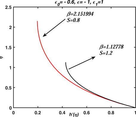
FIGURE 1. Two profiles of h′(η) or axial velocity are graphed for two different values of β and S. Note that the parameter β and S are used by Anderson et al. (Andersson et al., 2000) and the graphs are exactly matched with the published work of them. Moreover, these profiles are obtained from the numerical solution of Eqs. 17, 18 for the parameters values given in the title of this figure. These profiles are also reported in papers (Wang, 1990; Dandapat et al., 2003; Liu and Andersson, 2008).

3.2 General analysis of the numerical solution of Eq. 17 and Eq. 18 and evaluation of the shear stress

The simulated problem in Eq. 17 and Eq. 18 contains seven parameters and each of them is corresponding to some physical settings, therefore, different values have been assigned to these parameter and they are associated with multiple functions of some physical activity. So effects of all these parameters have been observed on the axial velocity component and shear stress at the surface of the plate. The shear stress is usually expressed by τ and generally defined for two dimensional flow as $\tau =\mu (\frac{\partial u}{\partial y}+\frac{\partial v}{\partial x})$, where μ, u and v are defined earlier. By substituting values of u and v from Eq. 4, whereas, the values of p(x, t), q(x, t), f(x, t) and r(x, t) are expressed in Eq. 11 and Eq. 12 and finally the shear stress τ is obtained as $\tau =\mu \frac{p(x,t)}{r(x,t)}{g}^{\prime }(\eta )$. The shear stress at the wall and its dimensionless form gives the skin frictions coefficient, which is obtained at the sheet of non-uniform thickness as: $g^{\prime }(0)=\frac{r(x,t)}{\mu p(x,t)}\tau {|}_{y=f(x)}$. From Eq. 14, we get: $g(\eta )=-\frac{1}{A_1{A}_2{\delta }_2}{h}^{\prime }(\eta )$ then the skin friction becomes $-\frac{1}{A_1{A}_2{\delta }_2}{h}^{″}(0)=\frac{r(x,t)}{\mu p(x,t)}\tau {|}_{y=f(x)}$ and after scaling it, we have, i.e., $-h^{″}(0)=\frac{r(x,t)}{\mu p(x,t)}{A}_1{A}_2{\delta }_2\tau {|}_{y=f(x)}$.

4 Graphs of the numerical solution and their discussion

In this paper, we have simulated the thin film flow over a porous and moving sheet of non-uniform thickness. At the first place, we introduced new function for the velocity components, and they have been strictly changed with the similarity variable. In the later stage, we imposed certain conditions on the boundaries inputs and field variables, defined at the free surface and on the face of the plate. In such situations, we obtained multiple set of ODEs (problems) along with boundary conditions, however, we explained only those cases which give the exact self similar problem. As a result, a special case has been appeared, and is converted easily into the classical cases of thin film flows under certain constraints on the parameters. Moreover, this special situation of the present simulation has been shown in Eq. 17 and Eq. 18, whereas, the system is solved numerically for different choices of the parameters value. Note that each set of specific value of the parameters represents some proper physical senario; Figure 2; Figure 3; Figure 4 Figure 5; Figure 6) show the profiles of axial velocity against the similarity variable, which are obtained from the numerical solution of Eq. 17 and Eq. 18, whereas, the profiles in these figures are drawn for different values of γ₂ (injection/suction), γ₁ (stretching/shrinking), ϵ₀ (deformation of boundary layer) and ϵ (deformation of thin film via deformation of boundary layer). The deformation (both expansion and squeezing can be take place) of both thin film and sheet have been measured in term of deformation of the boundary layer, whereas, the self or direct deformation of thin film through some external stresses has played significant role during the flow process. In Figure 3A, the squeezing of the boundary layer and sheet have been considered and the flow is maintained over a stretching sheet. Note that the pure (over all) expansion and squeezing cases have been discussed for the flow over a stretching (shrinking) and porous sheet. The term over all deformation (squeezing or contraction) has been used for the simultaneous deformation (squeezing or contraction) of the boundary layer, thin film and that of the sheet. Moreover, the film is deformed (squeezed and expanded) in two different ways (i) deformation due to boundary layer and deformation due to other external stresses. Note that the velocity profiles in Figure 2 are decreased (increased) against η and different values of γ₂, whereas, the increasing (decreasing) behaviour of the velocity profiles is observed against η for injection (suction). The profiles have been risen suddenly (gradually) and dropped in case of expansion (contraction) of film and boundary layer for both stretching and shrinking sheet flows. However, massive injection occurs through the porous sheet and stretching velocity of the sheet is taken in these observations. In this Figure 2, effects of injection and suction are seen on the axial velocity and it has changed uniformly with the variation of this parameter. It is worthy noticeable that thin film is expanded by two means in this situation 1) external stresses 2) deformation of boundary layer. Moreover, for different values of γ₂, the axial velocity at the free surface of thin film gives non-uniform values, whereas, it remains fixed, i.e., zero at the sheet for each value of γ₂. Note that for non-zero value of ϵ₀ (when the boundary layer deforms), the profiles of h′(η) intersect in between the free surface and plate, whereas, the common point is moving to left and right, depending upon the values of the parameters (see Figure 4; Figure 5). The large negative values of ϵ₀ show that the boundary layer has compressed extremely towards sheet. On the other hand, ϵ₀ measures the deformation of the boundary layer, which may expand and compressed simultaneously. Similarly ϵ measure deformation of the thin film and depends upon the boundary layer. Finally ϵ₁ defines deformation of sheet and it depends on the deformation of thin film. Remember that the nature of velocity is changed from increasing (decreasing) to decreasing (increasing) with the variation of parameters. The profiles in Figure 3 are decreased (increased) against η and different values of γ₂ (both injection and suction cases are taken). The increasing (decreasing) behaviour of the velocity profiles is observed against η for injection (suction) in these plots. Each profiles in these figures is increased and decreased gradually, whereas, it is increased suddenly and the profiles have shown boundary layer patterns for large injection and expanded boundary layer when the flow is maintained over an expanded and contracting sheet. The profiles in Figure 4A,B have shown increasing (decreasing) behaviour against η for γ₁ < 0 (γ₁ > 0). In these two plots, the analysis has carried out for the expanded flow of thin film with suction and injection. Moreover, an overshoot in the velocity profiles is observed at Figure 4C,D for γ₁ < 0 and ϵ₀ > 0. Note that the overshooting values have been seen increased (decreased) for large suction (deformation). Note that the overshoots in the profiles are observed for the flow over a compressed sheet. The velocity profiles are decreased against η in Figure 5 for the flow over a non-stretching (non-shrinking) sheet with an injection velocity. In Figures 5A,B the boundary layer shrinking is compressed more rapidly, and no stretching is taken into account and the sheet is equipped with injection velocity, whereas, in Figure 5C,D, injection is combined with stretching and shrinking. In Figures 5A,B, the velocity is decreased from zero to some fixed value against η, whereas, it is increased in the vicinity of plate and then decreased uniformly against η. In Figure 4; Figure 5, the profiles have a common point of intersection between the interval (0, 1) on η − axis, whereas, the profiles are linear (non-linear) on the left (right) of point of intersection and the graphs have shown asymptotic behavior on the right of the point. Moreover, the part of profiles on the left (right) are increased or decreased suddenly (gradually) against η. The reason is that the injection and expansion (which supports the injection) of sheet are assisting the flow in normal direction, whereas, the viscous nature of the fluid reduces or slow downs the impact of injection, and the velocity adopts non-linear nature after the point of intersection. In some cases overshoots in the velocity profiles have been seen and it is obvious fact that injection supports the flow in the normal direction. Note that the response of h′ to γ₁ between zero and the point of intersection is opposite to the response between the point of intersection and 1. In Figures 4A–D, the point of intersections for different values of γ₁ are (0.42857, 0.50282), (0.40816, 4.1703), (0.5102, −8.7341), (0.58163, −11.5064), respectively, whereas, the point of intersection moves, this means that it varies depending upon the value of the parameters. Note that for certain ranges of the parameters value, the point of intersection disappears as shown in Figures 4A–D. In Figures 5A–D, the point of intersections for ϵ₀ and γ₁ are (0.4898, −8.4287), (0.45918, −13.881), (0.42857, −11.1422), (0.42857, 1.0577), respectively, whereas, the point of intersection moves, this means that it depends upon the set of parameters values. The profiles in these two figures, i. e., Figure 4; Figure 5) have shown the linear (non-linear), increasing (decreasing) and asymptotic behaviors against γ₁ and ϵ₀ before (after) point of intersection. It is observed that the point of intersection moves to the right/left and upward (downward) with the changes in the parameters value who supported (resisted) injection. Note that the surface deformation has played significant role in supporting and opposing the injection rate.

FIGURE 2

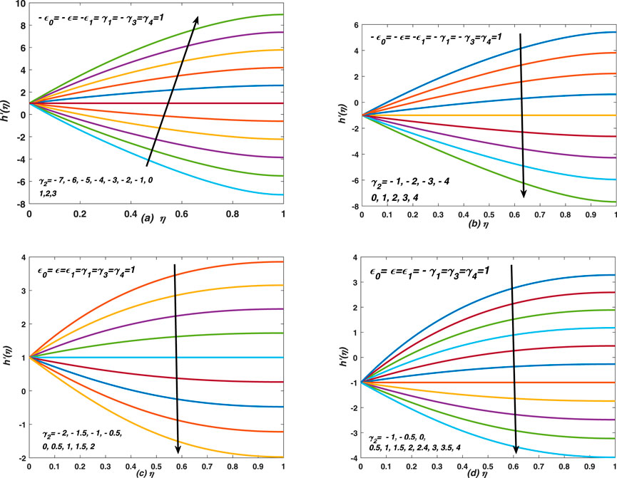
FIGURE 2. Flow behaviour of thin film has observed when the sheet, boundary layer and film are either compressed or expanded simultaneously. (A) Velocity profiles of squeezed flow of thin film have been graphed for the flow over a stretching sheet with suction and injection through its surface. (B)Velocity profiles of squeezed flow of thin film have been graphed for the flow over a shrinking sheet with suction and injection through its surface. (C) Velocity profiles of expanded flow of thin film have been graphed for the flow over a stretching sheet with suction and injection through its surface. (D) Velocity profiles of expanded flow of thin film have been graphed for the flow over a shrinking sheet with suction and injection through its surface.

FIGURE 3

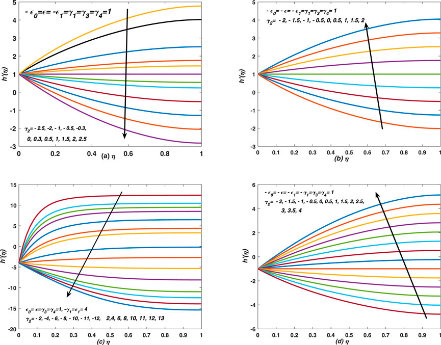
FIGURE 3. Flow behaviour of thin film has observed when the boundary layer is expanded/compressed with the deformation of film and sheet. (A) The axial velocity of deforming (both contraction and expansion can take place) thin film has been studied over a porous, stretched and compressed sheet in the presence of squeezed boundary layer. (B) Velocity profiles of thin film flow are drawn for flow over a stretching and porous sheet, whereas, the boundary layer is compressed. As a consequence, the sheet and thin film are also squeezed. Furthermore, the thin film is expanded via external stresses. (C) Velocity profiles of expanded flow of thin film are graphed for the flow over a shrinking sheet with suction and injection through its porous surface. (D) Velocity profiles of thin film flow are drawn for the flow over a shrinking and porous sheet, whereas, the boundary layer is compressed. As a consequence, the sheet and thin film are also squeezed. Furthermore, the thin film is expanded via external stresses.

FIGURE 4

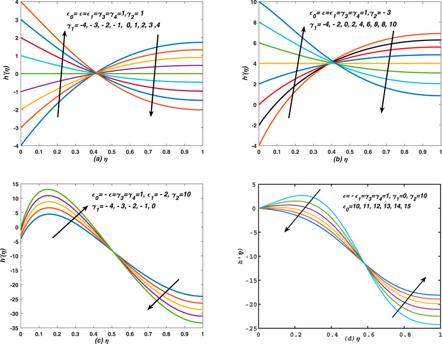
FIGURE 4. Flow bahaviour of thin film has observed for different values of (i) stretching/shrinking parameters and (ii) sudden expansion of the boundary layer. (A) Velocity profiles of expanded flow of thin film are graphed for the flow over a stretching and shrinking sheet with injection through porous plate. (B) Velocity profiles of expanded flow of thin film are graphed for the flow over a stretching and shrinking sheet with suction through porous plate. (C) An over shoot in the velocity profiles of deformed thin film flow has observed near the surface of the sheet. The sheet is compressed, whereas, the thin film is squeezed via external stresses. (D) Effects of boundary layer’s expansion of thin film and squeezing of sheet are seen on the axial velocity of thin film flow over a non-stretching(non-shrinking) sheet with the injection velocity through the plate.

FIGURE 5

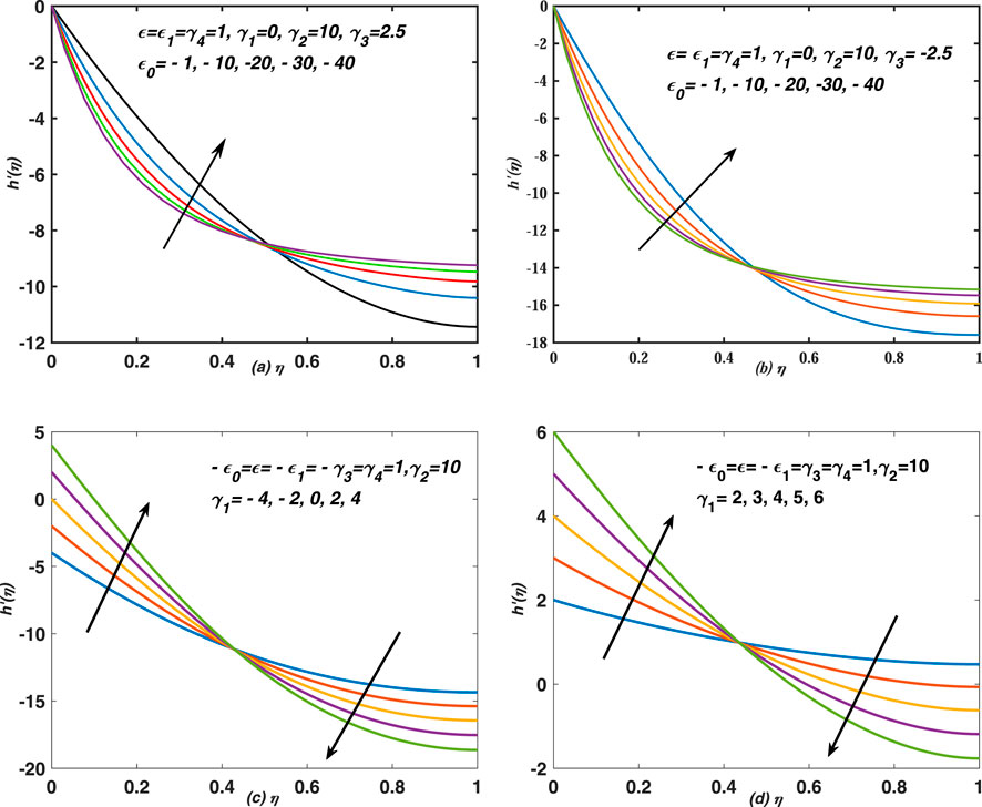
FIGURE 5. Decreasing behaviour of velocity profiles is observed against η for different values of (i) γ₁ (ii) ϵ₀ < 0 (sudden compression of boundary layer).(A) Effects of boundary layer’s compression and expansion of both thin film and sheet are seen on the axial velocity of thin film flow over a non-stretching (non-shrinking) sheet with the injection velocity through plate. (B) Effects of boundary layer’s compression, deformation of thin film and expansion of sheet are seen on the axial velocity of thin film flow over a non-stretching (non-shrinking) sheet with the injection velocity through the plate. (C) Effects of shrinking are seen on the axial velocity of thin film flow over a non-stretching (non-shrinking) sheet with the injection velocity through the plate. (D) Effects of stretching are seen on the axial velocity of thin film flow over a non-stretching (non-shrinking) sheet with the injection velocity through the plate.

FIGURE 6

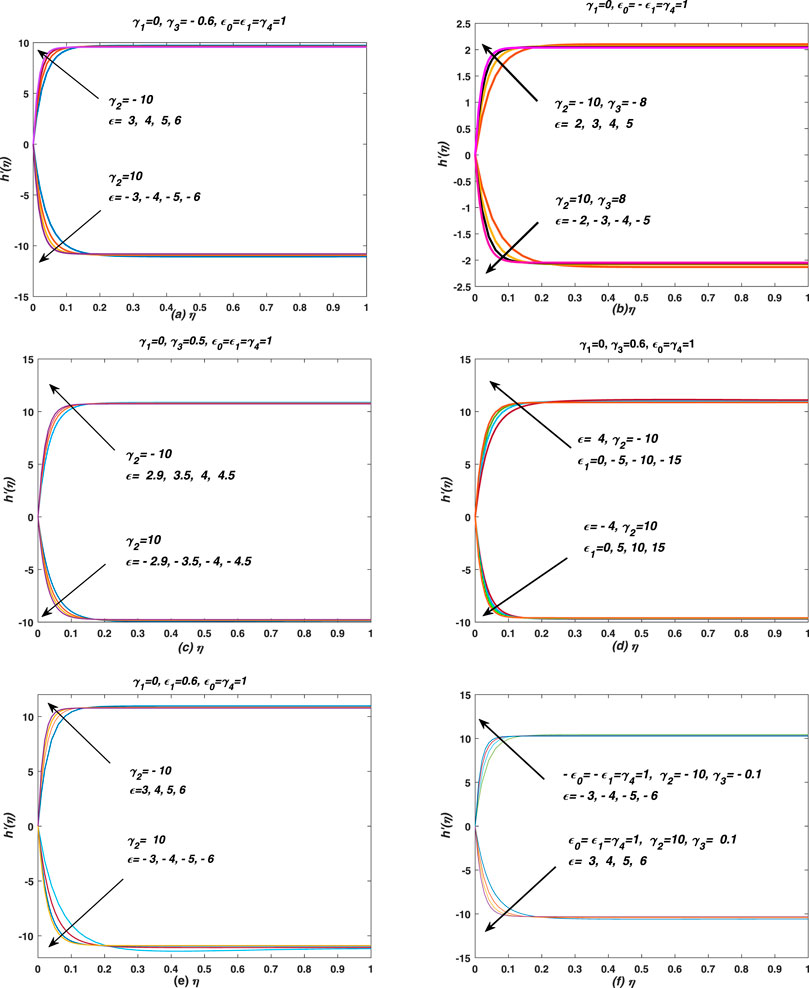
FIGURE 6. The boundary layer behaviour of thin film flow has observed when the flow is maintained over a non-stretching(γ₁ = 0)/non-shrinking sheet. (A) The film is expanded (γ₃ > 0)/compressed (γ₃ < 0) slowly by external stresses and it is expanded (ϵ > 0)/squeezed(ϵ < 0) via boundary layer. Note that the upper (lower) set of profiles is drawn for expanding sheet/boundary-layer and suction (injection) cases. (B) The film is expanded (γ₃ > 0)/compressed (γ₃ < 0) quickly by external stresses and it is expanded (ϵ > 0)/squeezed(ϵ < 0) via boundary layer. Note that the upper (lower) set of profiles is drawn for contracted sheet (ϵ₁ < 0), expended boundary-layer (ϵ₀ > 0) and suction (injection) cases. (C) The film is expanded (γ₃ > 0)/compressed (γ₃ < 0) by external stresses and it is expanded (ϵ > 0)/squeezed(ϵ < 0) via boundary layer. Note that the upper (lower) set of profiles is drawn for expanding sheet/boundary layer and suction (injection) cases. (D) The film is expanded (γ₃ > 0) by external stresses and it is expanded (ϵ > 0)/squeezed(ϵ < 0) via boundary layer. Note that the upper (lower) set of profiles is drawn for contracting (expanding) sheet and suction (injection) cases. (E) The film is squeezed (γ₃ < 0)/expanded (γ₃ > 0) by external stresses and it is expanded (ϵ > 0)/squeezed(ϵ < 0) via boundary layer. Note that the upper (lower) set of profiles is drawn for suction (injection) case. (F) The upper(lower) set of profiles is drawn for squeezing(expanding) and suction(injection) cases.

In Figure 6, the velocity profiles are asymptotic near the free surface for large injection/suction in the presence of squeezing (expanded) thin film flow, maintained over a non-stretching and non-shrinking sheet. Note that overshoot in velocity profiles is observed near the surface of plate for large shrinking (quick expansion of boundary layer) over a sheet with injection in case of expanding film (see Figures 4C,D). It happens because the injection provides extra momentum to the flows. Moreover, the film and surface deformations have minimum effect on the flow behaveiour in this special circumstances. The profiles of axial velocity in Figure 5A,B showed odd behavior, however, in case of squeezing film, the velocity profiles have been dropped more rapidly for compressing thin films as compared to its profile for expanding thin film. Furthermore, these observations are recorded in Figure 6A–D. Note that in all subplots of Figure 6, the boundary layer gets thinner and steaks to the sheet, whereas, it penetrates more quickly in case of squeezing thin film flow over an impermeable, shrinking and expanding sheet and these observations are noted in Figure 6E. A thin boundary layer is observed near the surface of the permeable (injection case) and non-stretching non-shrinking sheet, whereas, the boundary thickness is increased in case of flow over an impermeable and non-stretching and non-shrinking plate.On the other hand, Figure 7; Figure 8; Figure 9 show the profiles of skin friction against ϵ₀ (the boundary layer expansion and compression are taken) for different values of ϵ (both expansion and squeezing of thin film via boundary layer are considered) in the presence of deformation of thin films. Note that the profiles are drawn for the flow over a non-stretching and non-shrinking sheet with injection. The profiles are linear for squeezed and expanded thin film, whereas, they are decreased non-linearly against ϵ₀ when the expanding thin film is moved rapidly. On the other hand, the profiles are straight lines for expansion of film via external stresses through the boundary layer in the presence of shrinking sheet and they are decreased linearly. Furthermore, the experiment is repeated and the skin friction coefficient is graphed against ϵ₀ (compressed boundary layer is taken) for different values of stretching, shrinking and deformation of walls in Figure 8. In all these figures, the profile of skin friction are decreased rapidly and non-linearly against suction. In Figure 9A the skin friction is decreased linearly and quickly against injection for large stretching in case of expanding film. Whereas, the profiles are increased quickly and non-linearly against shrinking for abrupt expansion of surface in case of squeezing film. Moreover, the profiles are converge to a fixed value (i.e. 10) in each case and they converged asymptotically to 100 against ϵ. Finally, the profiles exhibit increasing (decreasing) behaveiour against ϵ₁ (ϵ) for non-stretching and non-shrinking plate, uniform boundary layer and rapid expansion of the boundary, respectively. In Figure 9B, the skin friction shows increasing and decreasing behaveiour against ϵ (expanding film) and ϵ₁ (expanding sheet) respectively. The profiles are decreased (increased) non-linearly for different values of ϵ and ϵ₁ in these two subplots. Note that the profiles show divergent behavior against ϵ₁ for small values of it (weak expansion of thin film) and they varied linearly against ϵ₁ for large values of it (expansion of thin film).

FIGURE 7

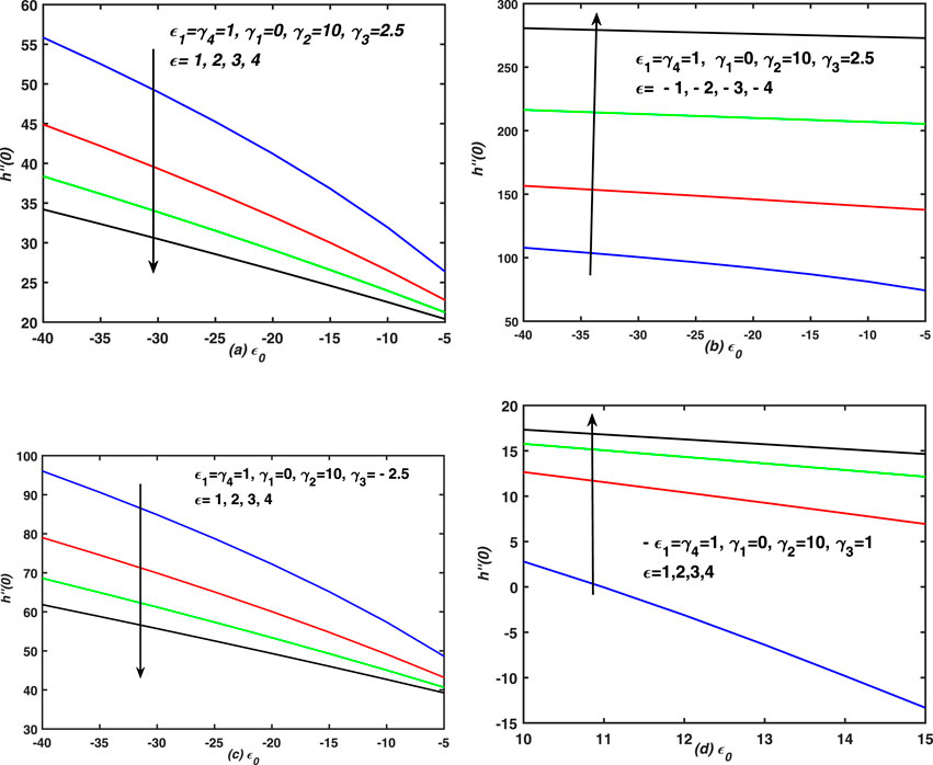
FIGURE 7. The linear and non-linear behaviour of skin friction is graphed against the compressed and expanded boundary layers. Note that the stretching and shrinking velocities are taken zero in this case. (A) Skin friction coefficient is plotted against compressed boundary layer (ϵ₀) for different values of expansion of thin film ϵ. It is the case of expanding film and injection through plate. (B) Skin friction coefficient is plotted against compressed boundary layer (ϵ₀) for different values of expansion of thin film ϵ. It is the case of deforming film and injection through plate. (C) Skin friction coefficient is plotted against compressed boundary layer (ϵ₀) for different values of expansion of thin film ϵ. It is the case of squeezing film and expanding plate with injection. (D) Skin friction coefficient is plotted against compressed boundary layer (ϵ₀) for different values of expansion of thin film ϵ. It is the case of expanding film and squeezing plate with injection.

FIGURE 8

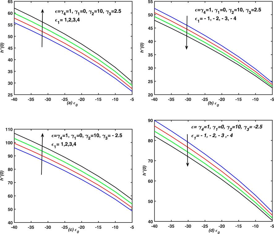
FIGURE 8. The linear and non-linear behaviour of skin friction is graphed against the compressed boundary layers. (A) Skin friction coefficient is plotted against compressed boundary layer (ϵ₀) for different values of deformation of sheet ϵ₁. It is the case of expanding film and injection through sheet. (B) Skin friction coefficient is plotted against compressed boundary layer (ϵ₀) for different values of deformation of sheet ϵ₁. It is the case of deforming film and injection through sheet. (C) Skin friction coefficient is plotted against compressed boundary layer (ϵ₀) for different values of deformation of sheet ϵ₁. It is the case of squeezing film and injection through sheet. (D) Skin friction coefficient is plotted against compressed boundary layer (ϵ₀) for different values of deformation of sheet ϵ₁. It is the case of squeezing film and injection through sheet.

FIGURE 9

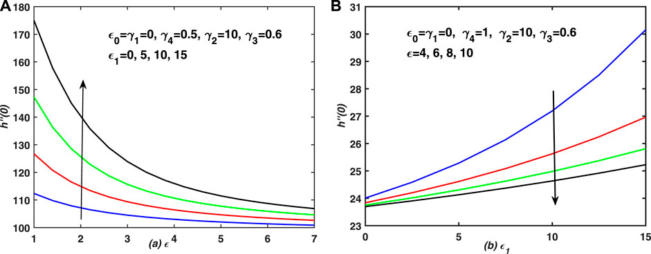
FIGURE 9. The increasing, decreasing and behaviour of skin friction is graphed against the expansion of sheet/thin film for different cases of expanding of thin film/sheet. (A) Skin friction coefficient is plotted against the expansion of sheet (ϵ) for different values of deformation of sheet ϵ₁. It is the case of expanding film and sheet with injection. (B) Skin friction coefficient is plotted against the expansion of sheet (ϵ₁) for different values of deformation of sheet ϵ₁. It is the case of expanding film and sheet with injection.

5 Conclusion

In this paper, we analyzed the flow of viscous thin film over a variably porous and moving sheet of non-uniform thickness. The non-uniform nature of thin film and thickness of the porous and moving sheet are major aspects of the present simulated flow model. The continuity law and boundary layer momentum equation are simplified in view of the generalized boundary conditions, imposed at sheet and free surface of thin film. A set of new variables is introduced for the velocity components and similarity variables, whereas, multiple constraints have been imposed on the set of transformations and they consequently provided multiple problems of self similar nature. A special case is formed from this transformation which is then converted into the classical problem for specific choice of the parameters value. So the results are exactly matched with the published work of (Wang, 1990; Andersson et al., 2000; Dandapat et al., 2003; Liu and Andersson, 2008). Moreover, the detailed discussion of this special case is also provided in view of new transformation. The problem is classified into several cases in which both steady and unsteady behaviors of the problem have been studied, whereas, the additional information and observation are also obtained from the present investigations. However, we restrict ourselves only to one case due to the length of the paper. Moreover, combined and individual effects of injection, suction, stretching, shrinking, deformation of both thin film and sheet have been seen on the axial velocity and skin friction. A narrow momentum boundary layer is observed over an permeable non-stretching and non-shrinking and expanding sheet of non-uniform thickness for the flow of thin film. Moreover, linear, non-linear, uniform, non-uniform, both sudden and gradual increasing and decreasing responses of the skin friction are observed for the different types of the boundary inputs. In nut shell three types of deformations are focused in this investigations, i.e., deformation of thin film, sheet and boundary layer. Moreover, two types of variations have been observed in the thickness of thin film. One is due to the surface stresses, whereas, the second one appears due to the changes in boundary layer. Significant changes in the flow behavior have been noted due to the variation of thin film, boundary layer and sheet thicknesses and these observations have been recorded in different graphs.

Data availability statement

The raw data supporting the conclusions of this article will be made available by the authors, without undue reservation.

Author contributions

There are three authors in this manuscript and each one has contributed properly. The mathematical model has been proposed by DK, all the numerical computations and their graphs have been carried out by NU. The discussion of graphs and their physical interpretation has been given by DK and ZK. The literature review and comparison of the present simulations with the classical data has been established by NU. The final review and amendments in the manuscript has been carried out by ZK.

Acknowledgments

Princess Nourah bint Abdulrahman University Researchers Supporting Project number (PNURSP 2023R8). Princess Nourah bint Abdulrahman University Riyadh, Saudi Arabia.

Conflict of interest

The authors declare that the research was conducted in the absence of any commercial or financial relationships that could be construed as a potential conflict of interest.

Publisher’s note

All claims expressed in this article are solely those of the authors and do not necessarily represent those of their affiliated organizations, or those of the publisher, the editors and the reviewers. Any product that may be evaluated in this article, or claim that may be made by its manufacturer, is not guaranteed or endorsed by the publisher.

References

Abbas, Z., Hayat, T., Sajid, M., and Asghar, S. (2008). Unsteady flow of a second grade fluid film over an unsteady stretching sheet. Math. Comput. Model. 48 (3-4), 518–526. doi:10.1016/j.mcm.2007.09.015

CrossRef Full Text | Google Scholar

Ali, A., Marwat, D. N. K., and Ali, A. (2022). Analysis of flow and heat transfer over stretching/shrinking and porous surfaces. J. Plastic Film Sheeting 38 (1), 21–45. doi:10.1177/87560879211025805

CrossRef Full Text | Google Scholar

Andersson, H. I., Aarseth, J. B., Braud, N., and Dandapat, B. S. (1996). Flow of a power law fluid film on an unsteady stretching surface. J. Newt. Fluid Mech. 62 (1), 1–8. doi:10.1016/0377-0257(95)01392-x

CrossRef Full Text | Google Scholar

Andersson, H. I., Aarseth, J. B., and Dandapat, B. S. (2000). Heat transfer in a liquid film on an unsteady stretching surface. Int. J. Heat Mass Transf. 43 (1), 69–74. doi:10.1016/s0017-9310(99)00123-4

CrossRef Full Text | Google Scholar

Burelbach, J. P., Bankoff, S. G., and Davis, S. H. (1990). Steady thermocapillary flows of thin liquid layers. II. Experiment. . Phys. Fluids A Fluid Dyn. 2 (3), 322–333. doi:10.1063/1.857782

CrossRef Full Text | Google Scholar

Chen, C. H. (2006). Effect of viscous dissipation on heat transfer in a non-Newtonian liquid film over an unsteady stretching sheet. J. Newt. Fluid Mech. 135 (2-3), 128–135. doi:10.1016/j.jnnfm.2006.01.009

CrossRef Full Text | Google Scholar

Crane, L. J. (1970). Flow past a stretching plate. Z. für Angew. Math. Phys. ZAMP 21 (4), 645–647. doi:10.1007/bf01587695

CrossRef Full Text | Google Scholar

Dandapat, B. S., Kitamura, A., and Santra, B. (2006). Transient film profile of thin liquid film flow on a stretching surface. Z. für Angew. Math. Phys. ZAMP 57 (4), 623–635. doi:10.1007/s00033-005-0040-7

CrossRef Full Text | Google Scholar

Dandapat, B. S., and Maity, S. (2006). Flow of a thin liquid film on an unsteady stretching sheet. Phys. fluids 18 (10), 102101. doi:10.1063/1.2360256

CrossRef Full Text | Google Scholar

Dandapat, B. S., and Ray, P. C. (1994). The effect of thermocapillarity on the flow of a thin liquid film on a rotating disc. J. Phys. D Appl. Phys. 27 (10), 2041–2045. doi:10.1088/0022-3727/27/10/009

CrossRef Full Text | Google Scholar

Dandapat, B. S., Santra, B., and Andersson, H. I. (2003). Thermocapillarity in a liquid film on an unsteady stretching surface. Int. J. Heat Mass Transf. 46 (16), 3009–3015. doi:10.1016/s0017-9310(03)00078-4

CrossRef Full Text | Google Scholar

Hussan, M., Mustafa, N., and Asghar, S. (2012). Mass transfer analysis for unsteady thin film flow over stretched heated plate. Int. J. Phys. Sci. 7 (12), 1903–1909. doi:10.5897/IJPS11.1674

CrossRef Full Text | Google Scholar

Krishna, M. V., Ahammad, N. A., and Algehyne, E. A. (2022). Unsteady MHD third-grade fluid past an absorbent high-temperature shrinking sheet packed with silver nanoparticles and non-linear radiation. J. Taibah Univ. Sci. 16 (1), 585–593. doi:10.1080/16583655.2022.2087396

CrossRef Full Text | Google Scholar

Liu, I. C., and Andersson, H. I. (2008). Heat transfer in a liquid film on an unsteady stretching sheet. Int. J. Therm. Sci. 47 (6), 766–772. doi:10.1016/j.ijthermalsci.2007.06.001

CrossRef Full Text | Google Scholar

Noor, N. F. M., Abdul-Aziz, O., and Hashim, I. (2010). MHD flow and heat transfer in a thin liquid film on an unsteady stretching sheet by the homotopy analysis method. Int. J. Numer. Methods Fluids 63 (3), 357–373. doi:10.1002/fld.2078

CrossRef Full Text | Google Scholar

Sakiadis, B. C. (1961). Boundary-layer behavior on continuous solid surfaces: I. Boundary-Layer equations for two-dimensional and axisymmetric flow. AIChE J. 7 (1), 26–28. doi:10.1002/aic.690070108

CrossRef Full Text | Google Scholar

Sakiadis, B. C. (1961). Boundary-layer behavior on continuous solid surfaces: II. The boundary layer on a continuous flat surface. AIChE J. 7 (2), 221–225. doi:10.1002/aic.690070211

CrossRef Full Text | Google Scholar

Santra, B., and Dandapat, B. S. (2009). Unsteady thin-film flow over a heated stretching sheet. Int. J. Heat Mass Transf. 52 (7-8), 1965–1970. doi:10.1016/j.ijheatmasstransfer.2008.09.036

CrossRef Full Text | Google Scholar

Siddiqui, A. A., and Turkyilmazoglu, M. (2022). Slit flow and thermal analysis of micropolar fluids in a symmetric channel with dynamic and permeable. Int. Commun. Heat Mass Transf. 132, 105844. doi:10.1016/j.icheatmasstransfer.2021.105844

CrossRef Full Text | Google Scholar

Sparrow, E. M., and Gregg, J. L. (1959). A boundary-layer treatment of laminar-film condensation. J. Heat Transf. 81 (1), 13–18. doi:10.1115/1.4008118

CrossRef Full Text | Google Scholar

Tan, M. J., Bankoff, S. G., and Davis, S. H. (1990). Steady thermocapillary flows of thin liquid layers. I. Theory. I. Theory. Phys. Fluids A Fluid Dyn. 2 (3), 313–321. doi:10.1063/1.857781

CrossRef Full Text | Google Scholar

Turkyilmazoglu, M. (2022). Asymptotic suction/injection flow induced by a uniform magnetohydrodynamics free stream couple stress fluid over a flat plate. J. Fluids Eng. 144 (3), 52417. doi:10.1115/1.4052417

CrossRef Full Text | Google Scholar

Turkyilmazoglu, M. (2022). Radially expanding/contracting and rotating sphere with suction. Int. J. Numer. Methods Heat Fluid Flow 32, 3439–3451. doi:10.1108/HFF-01-2022-0011

CrossRef Full Text | Google Scholar

Wang, C. (2006). Analytic solutions for a liquid film on an unsteady stretching surface. Heat Mass Transf. 42 (8), 759–766. doi:10.1007/s00231-005-0027-0

CrossRef Full Text | Google Scholar

Wang, C. Y. (1990). Liquid film on an unsteady stretching surface. Q. Appl. Math. 48 (4), 601–610. doi:10.1090/qam/1079908

CrossRef Full Text | Google Scholar

Nomenclature

α₁, α₂, α₃, α₄, α₅, α₆, α₇, α₈, α₉, α₁₀ variable coefficients

$\frac{\mathbf{D}}{\mathbf{D}\mathbf{t}}$ material time derivative

F dimensionless stream function

f(x, t) variable thickness of sheet

g(η) represent the velocity component v

h(η) represent the velocity component u

r(x, t) variable size of the thin film

S unsteadiness parameter

t time variable

u, v velocity components in x(y) directions

U stretching(shrinking) velocity

V injection(suction) velocity

w controlling parameter for the deformation of thin film

x, y Cartesian Coordinates

Greek letters

η similarity variables

τ shear stress

β value of similarity variable at the surface of thin film

ϵ₀ boundary layer deformation

ϵ deformation of thin film due to boundary layer

ϵ₁ deformation of sheet

γ₁ stretching and shrinking parameter

γ₂ injection and suction parameter

γ₃ dimensionless normal velocity at the surface of the film

γ₄ value of similarity variable at surface of thin film