 Syed Ibrahim
 Dil Nawaz Khan Marwat1
- 1Department of Mathematics, Islamia College Peshawar, University Campus, Peshawar, Khyber Pakhtunkhwa, Pakistan
- 2Riphah International University, Chakdara, Khyber Pakhtunkhwa, Pakistan
- 3Department of Mathematics, College of Science and Humanities in Alkharj, Prince Sattam Bin Abdulaziz University, Alkharj, Saudi Arabia
- 4School of Technology, Woxsen University, Hyderabad, India
Fluid flows occur due to internal or external forces such as wind, gravity, pressure gradients, side-wall motion, MHD, and free convection. This study examines how meanders impact heat transfer by studying the behavior of viscous fluid flow with streamwise vortices in a sinusoidal wavy meandering channel of non-uniform radius. The study simplifies the motion and energy equations governing the fluid flow using novel transformations and a regular perturbation method. By plotting graphs for different parameter values, such as Pr, Re, and Ec, it reveals that decreasing the wavelength leads to flow separation near the channel surface. However, the stream moves forward with a sudden meander disturbance, causing the flow to become rectilinear and independent of vertex-generating centrifugal forces. The study identifies a stream function using standard and established relations. The fluid flow patterns and temperature distribution behavior are shown in various plots, highlighting the significant impact of meanders on fluid flow.
1 Introduction
There are infinitely many possible types of meanders, and here we consider only a special type of meandering channel, i.e., the sinusoidal meandering channel. These channels are influenced by various agents that cause fluid motion, with the most common being the pressure gradient. In some cases, the pressure gradient may be mechanical in nature. The flows within these channels are predominantly induced by the pressure gradient, and they have numerous practical applications (Webb and Bergles, 1981; Bergles and Webb, 1985; Jensen et al., 1997; Ligrani et al., 2003). The partition of escalation structures can be performed on those that are responsible for necessary changes in the thermal and physical properties of fluids under consideration and the ones marked by perfection in fluid maxing (Fiebig, 1995a; Fiebig, 1995b; Jacobi and Shah, 1995). Mixing with improved mechanics is the point of attention in engineering devices functioning at small Reynolds numbers (Re) with laminar patterns (Fiebig, 1998). Commonly, it is understood that improved mixing can be done via compelling the fluid from the laminar state into a turbulent one or by the formation vortex generators. Vortex generators are functional but have significant pressure in their drag drawback (Patera and Mikic, 1986; Fiebig and Chen, 1999).
For nearly a century, centrifugal instability has been observed in shear layers. Previous studies focused on simple geometries and canonical flows, making it easy to calculate the curvature or meander of flow patterns. One example is the flow of fluid motion between rotating cylinders, where (Floryan, 1991) investigated the stability states of the distribution of rotation in an inviscid mechanism. In (Mohammadi and Floryan, 2013), addressed a highly viscous problem was addressed, and the critical conditions of the secondary flow onset were determined. In (Xu et al., 2016), comparable instability in curved channels was analyzed, and (Rayleigh, 1917) presented a case of boundary layer flows on concave sheets, taking into account centrifugal instability. In (Taylor, 1923), it was found that the special type of instability is prominent for fluid flow over concave and convex sheets, subject to the condition that the velocity components are non-monotonic in nature. In (Ghalambaz et al., 2016; Hayat et al., 2017; Srinivasacharya and Sibanda, 2020; Mahmud and Uddin, 2021), numerical simulation and analysis of different types of nanofluids flowing past various types of surfaces in the context of fluid flow and heat transfer in different channels was performed (Khan and Ahmed, 2015; Alsaedi et al., 2016; Nadeem et al., 2016; Izadi and Pourmehran, 2017; Khan et al., 2017; Sheikholeslami et al., 2017). These studies explore the impact of various factors such as thermal radiation, magnetic fields, bioconvection, entropy optimization, and chemical reactions on flow and heat transfer characteristics. As such, these articles are highly relevant for those interested in studying the behavior of nanofluids. All of these results apply to constant meanders and establish a clear relationship between streamline meanders and the wall meander. Consequently, the demonstration of this special type of stability revealed that it is represented by a single parameter, which is one possible way to describe this meandering with a single parameter.
The main objective of this study is to investigate the flow of a viscous fluid in a meandering channel with wavy walls driven by a pressure gradient. The equations of motion, including the conservation of the mass and momentum equations and the energy equation, are utilized to analyze the fluid flow and temperature distribution within the channel. The boundary conditions are imposed on the channel walls and at the center of the channel to maintain symmetry. Dimensionless variables are used to transform the governing equations into a dimensionless form for easy tracking of units. Additionally, the study explores special types of instabilities and their significance. In the first part, an assumption of fixed pressure gradient is imposed, assuming direct channel flow with parallel plates, and sinusoidal channel flow is driven by an identical pressure gradient. Flow rate variation is used to supplement the flow losses associated with the meandering channel. The generalized model is solved using perturbation method, and the stream function is calculated and examined using other techniques. The temperature distribution behavior is illustrated through various plots depicting different dimensionless parameters, such as Pr, Re, and Ec.
2 Geometry of the problem
Consider the flow of a viscous fluid in a meandering channel, which consists of two wavy walls separated by a fixed gap. The classical model for laminar flows in channels, tubes, and ducts is provided by Poiseuille. The flow in such a channel is primarily induced by a pressure gradient. There are various types of flows that pass through ducts and channels, and they have significant practical importance. The classification of scaling structures can be conducted based on those that have variations in the effective thermophysical properties of fluids, and the pursuit of optimal fluid mixing can lead to an infinite number of possible meander types. In this study, we will focus on the simplest sinusoidal channel, whose geometry is illustrated in Figure 1, where the superscript H denotes the upper and G denotes the lower walls of the channel. The channel extends along the x-axis from negative infinity to positive infinity, and the flow is driven by a pressure gradient.

FIGURE 1. Geometry of meandering channel and flow field under consideration.
3 Governing equations and their non-dimensional form
The general form of continuity equation for incompressible viscous flow is:
The velocity vector, denoted as V, has three components for three-dimensional flow. Similarly, the general form of the Navier–Stokes equations applies to steady and viscous flows of constant viscosity.
The variables ρ, μ, and P represent density, viscosity, and pressure of the fluid, respectively. To define the dimensionless variables, we use asterisks and reference length L and velocity U, as follows:
After substituting the non-dimensional variables, which are defined in Eq. 3, into Eqs 1, 2, we obtain the dimensionless continuity and Navier–Stokes equations:
The above equation is multiplied by
where
4 Modeling of the problem
Let us consider that for flow in a straight channel and for two-dimensional flow, the velocity is represented by the velocity
The
The
The boundary conditions for the problem are established by utilizing the no-slip condition, along with considering the geometry of the problem. Thus, the boundary conditions can be written as:
Equations 7–9 represent the continuity and the
Note that Eqs 1–11 for the fully developed flow in a straight channel has been reported in F.M. White [31] and Schlichting [32].
The volume flow rate for the channel flow of fixed width is:
The stream function
In a meandering channel, where the fluid flow moves in the positive x-axis direction, the Reynolds number is defined based on the maximum x-velocity and channel half-height.
The velocity field and other related field quantities for the fluid motion in the meandering channel can be expressed as follows:
In the context of the meandering channel geometry, the velocity
This is achieved by substituting the new variables for the velocity field in the dimensionless governing equations, i.e., Eqs 4, 6, and eliminating pressure term.
The continuity equation Eq. 4 in the new variable is:
and now using the decomposed forms of
Note that
The dimensionless
The dimensionless
The pressure term is eliminated by expending the terms
in Eqs 18, 19, and then by subtracting Eq. 19 from Eq. 18, we get:
We define a stream function (
Substituting in Eq. 20, we get:
From the above continuity Eq. 22, we have:
By substituting in Eq. 22, we have:
The no slip boundary conditions:
Reconsidering the total stream function:
Floryan (1997) used the Fourier expansion for the simplification of the above equation:
where
By substituting Eq. 27 into Eq. 24, we get:
where
The equations of the model are valid for a constant pressure gradient, where both the straight and sinusoidal channels are driven by the same gradient. The flow rate variation is taken into account and measured due to the extra flow losses that occur in the meandering channel. Additionally, it is assumed that in Eq. 26, A is equal to zero, and the correction for the flow rate,
5 Solution of the modified equations
Let us assume that the wavelength is a large quantity, denoted as
The no-slip boundary and free-stream conditions with the total flow rate given in Eq. 25 is reduced to the following simplest form:
In Eqs 30–32 are three unknown quantities, i.e.,
Substituting the values of
6 Analysis of heat transfer in a meandering channel
The analysis of heat transfer in a meandering channel involves studying the heat transfer mechanisms that occur due to meanders in the channel. Heat transfer occurs in three modes: conduction, convection, and radiation. In the present study, a case of heat transfer through conduction and convection is taken into account. Conduction occurs when heat flows from regions of high temperature to regions of low temperature through a solid material. In a meandering channel, heat is conducted through the walls of the channel. The rate of heat transfer through conduction is proportional to the temperature gradient, the thermal conductivity of the material, and the cross-sectional area of the channel. Convection occurs when heat is transferred by the movement of fluids, either liquids or gases. In a meandering channel, heat is transferred through convection due to the flow of fluid through the channel. The rate of heat transfer through convection is proportional to the temperature difference between the fluid and the channel wall, the velocity of the fluid, and the heat transfer coefficient of the fluid. The heat transfer is analyzed by using the energy equation, which relates the rate of heat transfer to the temperature distribution in the channel. The energy equation is taken into account to study the conduction and convection mechanisms of heat transfer and the thermal properties of the meandering channel in the flow of fluids.
7 Formulation of the problem
The problem is modeled using the Navier–Stokes equations, along with the continuity and energy equations. To obtain a non-linear, simple partial differential equation, a defined set of transformations is applied. The regular perturbation technique is utilized to expand the heat transfer,
The energy equation is:
where
Consider the following dimensionless variables in order to transform the energy equation into dimensionless form:
The dimensionless numbers that appear in Eq. 38 are the Reynolds and Prandtl numbers, which are defined as:
Equation 41 is the dimensionless form of the energy equation. On the other hand, the boundaries conditions for the temperature distribution in the dimensionless form are obtained, and the dimensional boundary conditions are given by taking:
The temperature at the upper wall is
The temperature at the lower wall is
The temperature of a flow in a straight channel is denoted by
The boundaries condition for the temperature at the upper wall,
Putting Eq. 11 into Eq. 45, after simplification we have:
Integrating Eq. 46 twice w.r.t
where
As the
It is assumed that
We get:
The boundaries condition on the upper wall is
8 Results and discussion
With the solution represented as a power expansion in terms of
And
Stream function
The stream function
By integrating
The streamlines in the area adjacent to the lower wall are shown in Figures 2A, B, where
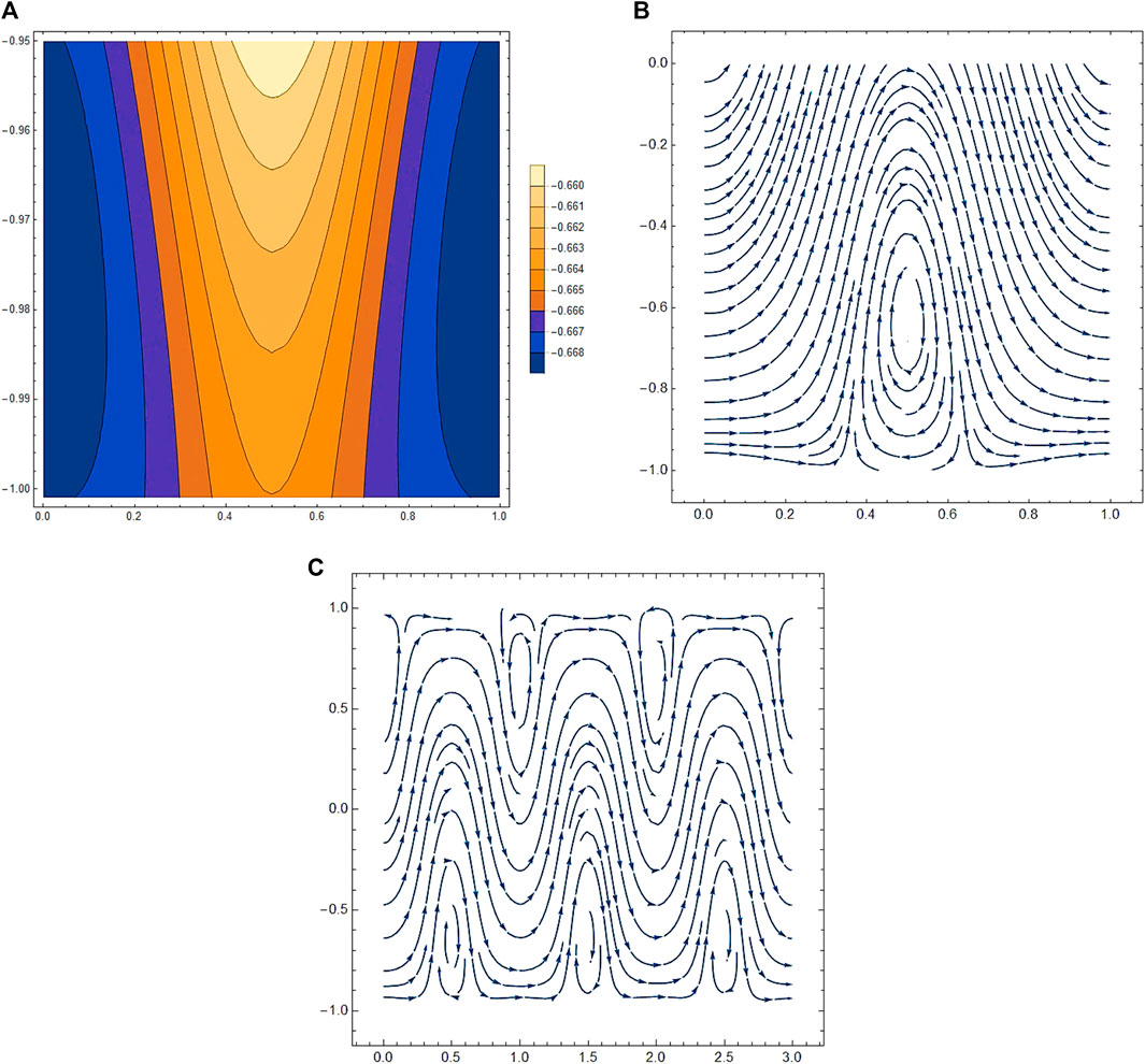
FIGURE 2. The streamlines in the area adjacent to the lower wall are shown in (A,B) where S = 5 (amplitude), Re = 1, and α = 10, while (C) is plotted for the whole channel.
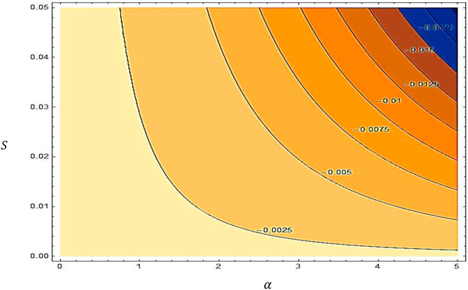
FIGURE 3. Variations of the pressure gradient correction Re[(dP_1)/dx] = -0.002.
9 Conclusion
The periodicity of the meandering channel affects the flow pattern and turbulence intensity of the fluid. A higher periodicity leads to a more regular flow pattern, while a lower periodicity leads to a more chaotic flow pattern. The presence of periodicity also leads to the development of secondary flows, such as Dean vortices, which affect the mixing and heat transfer characteristics of the flow. The Prandtl number relates the momentum diffusivity to the thermal diffusivity of a fluid. In a meandering channel, a higher Prandtl number results in a thicker thermal boundary layer, which affects the heat transfer characteristics of the flow. A lower Prandtl number, on the other hand, results in a thinner thermal boundary layer and a more efficient heat transfer. As shown in the Figures 4–8, the Eckert number relates the kinetic energy of a fluid to its thermal energy. In a meandering channel, a higher Eckert number results in a more energetic flow, which can lead to an increase in turbulence intensity and mixing. A lower Eckert number results in a less energetic flow, which leads to a more laminar flow pattern and reduced mixing. The Reynolds number represents the inertial forces to the viscous forces in a fluid. In a meandering channel, a higher Reynolds number results in a more turbulent flow pattern, with increased mixing and heat transfer. A lower Reynolds number results in a more laminar flow pattern, with reduced mixing and heat transfer. The effects of periodicity and the Prandtl number, Eckert number, and Reynolds number on fluid flow in a meandering channel are complex and interrelated.
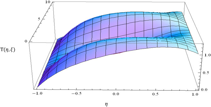
FIGURE 4. Temperature distribution is uniform and smooth from 0 to 1 in the direction of η, whereas its behavior in ξ direction is periodic in nature. For fixed values of S = 0.0125, Re = 10, α = 0.1, Pr = 1, and Ec = 1.
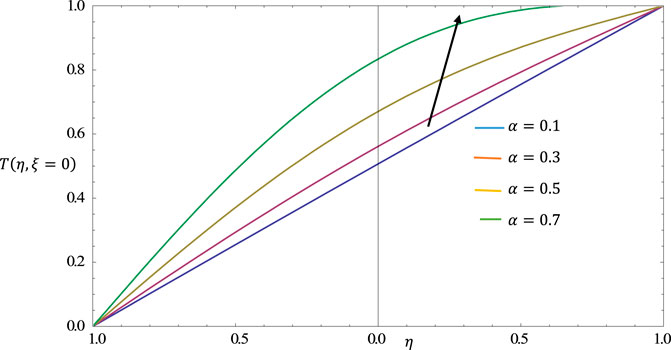
FIGURE 5. Temperature distribution
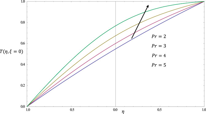
FIGURE 6. Temperature distribution
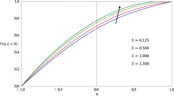
FIGURE 7. Temperature distribution
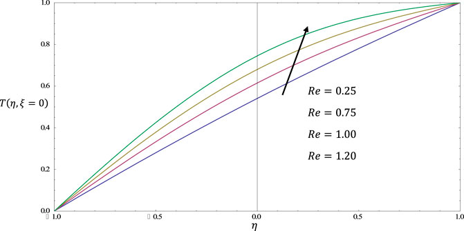
FIGURE 8. Temperature distribution
In future, the flow and heat transfer in wavy meandering channels could include investigating the thermal profiles, skin friction, and Nusselt number calculations for various flow parameters. This could provide insights into the heat transfer characteristics of the flow and help optimize the design of such channels for specific applications. Additionally, examining the effects of different geometries and materials on the flow and heat transfer could yield valuable results.
Data availability statement
The original contributions presented in the study are included in the article/Supplementary material, further inquiries can be directed to the corresponding author.
Author contributions
DK proposed the mathematical model. SI performed all numerical computations and created the corresponding graphs. DK and SI provided the discussion of the graphs and their physical interpretation. NU conducted the literature review and compared the present simulations with classical data. KN and K carried out the final review and made amendments to the manuscript.
Funding
This study was supported by funding from Prince Sattam bin Abdulaziz University, project number (PSAU/2023/R/1444).
Conflict of interest
The authors declare that the research was conducted in the absence of any commercial or financial relationships that could be construed as a potential conflict of interest.
Publisher’s note
All claims expressed in this article are solely those of the authors and do not necessarily represent those of their affiliated organizations, or those of the publisher, the editors and the reviewers. Any product that may be evaluated in this article, or claim that may be made by its manufacturer, is not guaranteed or endorsed by the publisher.
References
Alsaedi, A., Rashad, A. M., and Hayat, T. (2016). Bioconvective Darcy–Forchheimer flow of the Ree–Eyring nanofluid through a stretching sheet with velocity and thermal slips. J. Mol. Liq. 220, 803–811.
Bergles, A. E., and Webb, Ralph L. (1985). A guide to the literature on convective heat transfer augmentation. Ames, IA, USA: Iowa State University College of Engineering.
Fiebig, Martin, and Chen, Yuwen (1999). Heat transfer enhancement by wing-type longitudinal vortex generators and their application to finned oval tube heat exchanger elements. Heat Transf. Enhanc. Heat Exch. 42, 79–105.
Fiebig, Martin. (1995). Embedded vortices in internal flow: Heat transfer and pressure loss enhancement. Int. J. Heat Fluid Flow 16 (5), 376–388. doi:10.1016/0142-727x(95)00043-p
Fiebig, Martin. (1995). Vortex generators for compact heat exchangers. J. Enhanc. Heat Transf. 2, 1–20. doi:10.1615/jenhheattransf.v24.i1-6.10
Fiebig, M. (1998). Vortices, generators and heat transfer. Chem. Eng. Res. Des. 76 (2), 108–123. doi:10.1205/026387698524686
Floryan, J. M. (1991). On the Görtler instability of boundary layers. Prog. Aerosp. Sci. 28 (3), 235–271. doi:10.1016/0376-0421(91)90006-p
Ghalambaz, M., Rostami, B., and Rashidi, M. M. (2016). Thermal analysis of a radiative nanofluid over a stretching/shrinking cylinder with viscous dissipation. J. Mol. Liq. 224, 87–93.
Hayat, T., Ahmad, B., Alsaedi, A., and Rasool, N. (2017). Theoretical analysis of the thermal characteristics of Ree–Eyring nanofluid flowing past a stretching sheet due to bioconvection. J. Mol. Liq. 242, 758–764.
Izadi, M., and Pourmehran, O. (2017). Formation of hydrogen bonding during the Homann flow over a cylindrical disk of variable visco-elastic nano-materials in presence of activation energy. Int. J. Hydrogen Energy 42 (28), 18003–18016.
Jacobi, A. M., and Shah, R. K. (1995). Heat transfer surface enhancement through the use of longitudinal vortices: A review of recent progress. Exp. Therm. Fluid Sci. 11 (3), 295–309. doi:10.1016/0894-1777(95)00066-u
Jensen, Michael K., Bergles, Arthur E., and Shome., Biswadip (1997). The literature on enhancement of convective heat and mass transfer. J. Enhanc. Heat Transf. 4, 1–6. doi:10.1615/jenhheattransf.v4.i1.10
Khan, M., Saleem, S., and Rehman, K. U. (2017). Energy and mass transport through hybrid nanofluid flow passing over an extended cylinder with the magnetic dipole using a computational approach. J. Magnetism Magnetic Mater. 427, 107–114.
Khan, W. A., and Ahmed, S. (2015). Significance of activation energy and entropy optimization in radiative stagnation point flow of nanofluid with cross-diffusion and viscous dissipation. Results Phys. 5, 301–311.
Ligrani, Phil M., Oliveira, Mauro M., and Tim Blaskovich, (2003). Comparison of heat transfer augmentation techniques. AIAA J. 41 (3), 337–362. doi:10.2514/2.1964
Mahmud, S., and Uddin, M. J. (2021). Numerical simulations for optimised flow of second-grade nanofluid due to rotating disk with nonlinear thermal radiation: Chebyshev spectral collocation method analysis J. Therm. Analysis Calorim. 145 (2), 1087–1100.
Mohammadi, A., and Floryan, J. M. (2013) Groove optimization for drag reduction Phys. Fluids 25 (11), 113601 doi:10.1063/1.4826983
Nadeem, S., Akbar, N. S., and Lee, C. (2016) Numerical analysis of a time-dependent aligned MHD boundary layer flow of a hybrid nanofluid over a porous radiated stretching/shrinking surface J. Mol. Liq. 220, 945–954.
Patera, A. T., and Mikic, B. B. “Exploiting hydrodynamic instabilities. Resonant heat transfer enhancement” Int. J. heat mass Transf. 29 8 (1986): 1127–1138.doi:10.1016/0017-9310(86)90144-4
Rayleigh, Lord. (1917). On the dynamics of revolving fluids. Proc. R. Soc. Lond. Ser. A, Contain. Pap. a Math. Phys. Character 93 (648), 148–154.
Sheikholeslami, M., Rokni, H. B., and Ganji, D. D. (2017). Numerical investigation of Darcy–Forchheimer hybrid nanofluid flow with energy transfer over a spinning fluctuating disk under the influence of chemical reaction and heat source. J. Therm. Analysis Calorim. 128 (2), 913–924.
Srinivasacharya, D., and Sibanda, P. (2020). Investigation of hydromagnetic bioconvection flow of Oldroyd-B nanofluid past a porous stretching surface. J. Therm. Analysis Calorim. 139 (1), 237–247.
Taylor, Geoffrey Ingram. "VIII. Stability of a viscous liquid contained between two rotating cylinders." Philosophical Trans. R. Soc. Lond. Ser. A, Contain. Pap. a Math. or Phys. Character 223.605–615. (1923).
Webb, R. L., and Bergles, A. E. (1981). Performance evaluation criteria for selection of heat transfer surface geometries used in low Reynolds number heat exchangers. Ames, IA, USA: Iowa State University College of Engineering.
White, F. M., and Majdalani, J. (2006). Viscous fluid flow. New York, NY, USA: McGraw-Hill, 433–434.
Xu, Minghai, Lu, H., Gong, L., Chai, J. C., and Duan, X. (2016). Parametric numerical study of the flow and heat transfer in microchannel with dimples. Int. Commun. Heat Mass Transf. 76, 348–357. doi:10.1016/j.icheatmasstransfer.2016.06.002
Keywords: stream wise vortices, meandering channel, flow separation, instability, nonuniform radius
Citation: Ibrahim S, Khan Marwat DN, Ullah N, Nisar KS and Kamran (2023) Flow and heat transfer in a meandering channel. Front. Mater. 10:1183175. doi: 10.3389/fmats.2023.1183175
Received: 09 March 2023; Accepted: 29 May 2023;
Published: 26 July 2023.
Edited by:
Noor Saeed Khan, University of Education Lahore, PakistanReviewed by:
M. Riaz Khan, Quaid-i-Azam University, PakistanNilankush Acharya, Jadavpur University, India
Copyright © 2023 Ibrahim, Khan Marwat, Ullah, Nisar and Kamran. This is an open-access article distributed under the terms of the Creative Commons Attribution License (CC BY). The use, distribution or reproduction in other forums is permitted, provided the original author(s) and the copyright owner(s) are credited and that the original publication in this journal is cited, in accordance with accepted academic practice. No use, distribution or reproduction is permitted which does not comply with these terms.
*Correspondence: Syed Ibrahim, c3llZC5pYnJhaGltQHJpcGhhaC5lZHUucGs=