Analysis on intelligent deformation prediction of deep foundation pits with internal support based on optical fiber monitoring and the HSS model

1 Introduction

Deformation of foundation pits is the result of the interaction between the support structures and soil (Zheng et al., 2016). Considering the property of soil being of great complexity and diversity, it is a necessity to select reasonable soil constitutive model and parameters, which ensures the entire process of excavation of foundation pits is effectively simulated, so as to provide important technical support for the design of foundation pits as well as for construction safety (Zhao et al., 2016). The Hardening Soil model is an advanced constitutive model of soil, which takes the strain hardening characteristics of soft soil into account and regards the stress history and stress path as a significant basis for calculating soil stiffness. Furthermore, its deformation calculation results consider the combined action of foundation pit support structures and the surrounding soil (Zong and Xu, 2019). The variation pattern of soil stiffness can be classified into three kinds: very small strain (< 0.001%), small strain (0.001%–1%), and large strain (>1%) (Atkinson and Sallfors, 1991). Schweiger et al. (2009) studied a large amount of engineering monitoring data and found that, during the excavation process of foundation pits, most soil within the excavation range is in a state of small strain. As has been shown by numerous experiments, the deformation characteristics of soil mass under the small strain condition are fairly complicated and highly non-linear (Chen et al., 2021; Gu et al., 2021; Li et al., 2021; Zhang et al., 2022).

For the reasons given above, the Hardening Soil-small (HSS) model, taking the features of small strain of soil into consideration, was adopted to research the deformation trend of soil and support structures in foundation pit engineering, which improves the accuracy and rationality of the numerical analysis (Benz, 2007). Kim and Finno (2019) obtained the HSS model parameters of their research region through back-analysis of soil test results, and, by resorting to the sensitivity analysis of the model parameters at different stages of excavation, the parameters of the HSS model were optimized. Afterward, the researchers applied them to the numerical simulation of foundation pit deformation and then compared the derived data with the field measured values. The comparative results demonstrated that the HSS model can effectively predict the deformation of both side walls and the surface settlement of foundation pits. Wang et al. (2013) referred to plenty of experimental results and related studies, modified parameters $E_{50}^{\mathrm{r}\mathrm{e}\mathrm{f}}$, $E_{\mathrm{o}\mathrm{e}\mathrm{d}}^{\mathrm{r}\mathrm{e}\mathrm{f}}$, $E_{\mathrm{u}\mathrm{r}}^{\mathrm{r}\mathrm{e}\mathrm{f}}$, ${\gamma }_{0.7}$, and $R_{\mathrm{f}}$ via sensitivity analysis, calculated $G_0^{\mathrm{r}\mathrm{e}\mathrm{f}}$ through the back-analysis method, and finally concluded a set of preliminarily complete determining HSS model parameters on the basis of typical HS model parameters in Shanghai (Wang et al., 2012). Mu et al. (2012) acquired the HSS model parameters of the soil around a foundation pit via the back-analysis based on the coupling of MATLAB and Macro, and completed a numerical simulation of the construction process. They then compared and analyzed the change rule of the simulated value and the measured value. The comparative results indicated that the HSS model, considering the characteristics of small strain soil, can accurately adapt to the soil stiffness, which would effectively reduce the finite element calculation error of the next excavation. The rationality of the back-analysis method has been verified as well in the studies. Liang et al., 2017 obtained the main parameter values and their proportional relationships of the HSS model of typical clay layers in Shanghai through laboratory soil tests, and compared the calculated values and measured values of the deformation of the support structures based on foundation pit engineering examples. The study showed that the HSS model and the parameters gained from the test method are applicable to the simulation of foundation pit excavations in soft soil areas of Shanghai. Wu et al. (2021), on the basis of deep foundation pit engineering of typical soft soil in Shanghai, utilized Plaxis to establish a three-dimensional model according to the HSS model and corresponding parameters, carried out finite element analysis on the whole process of excavation, and studied the deformation of deep foundation pit excavations in the typical soft soil of Shanghai. This study delivered a technical reference for the design and construction of narrow-long deep foundation pits Shi et al. (2016) studied the stiffness parameters $E_{50}^{\mathrm{r}\mathrm{e}\mathrm{f}}$, $G_0^{\mathrm{r}\mathrm{e}\mathrm{f}}$, and ${\gamma }_{0.7}$ in the HSS model of typical soil layers in the Xiamen area, and the model’s sensitivity to the numerical simulation results of underground engineering. They sorted and compared the deformation sensitivity of each parameter at each stage of foundation pit excavation by using the single control soil layer parameters and orthogonal test method. This provides a reference point for the precise control of foundation pit deformation in the process of engineering investigations.

In summary, in contrast with the HS model, the HSS model takes into account the small strain characteristics of soil better, hence it is widely used in engineering issues such as foundation pit excavation. The HSS model, however, requires more parameters which are relatively difficult to obtain to characterize soil properties. Therefore, experimental methods or back-analysis is commonly adopted to achieve the parameters. On the other hand, the properties of soils in different regions may be various, so the correction and calibration of parameters in specific applications should align with the realistic situation of the region.

Foundation pit engineering monitoring refers to a procedure during foundation pit excavation, including monitoring the deformation of the foundation pit support structures and their surroundings using equipment and instruments, analyzing monitoring data to report results, and lastly comparing the results with alarm values to judge the excavation’s safety (Xi and Wei, 2020). Although some normal monitoring methods can be used for fixed-point monitoring of structural characteristics, they cannot precisely locate the local strain and relevant cracking, perform real-time monitoring on support structures, and realize the continuous measurement of strain, bending moment, and uneven settlement (Fu and Peng, 2018). In addition, point measurement frequency is not conducive to the timely discovery of dangerous situations to ensure the safety of the project and is subject to other disadvantages like adjacent buildings being possibly affected. This poses a huge challenge in preventing construction hazards. Wang N. et al., 2020 conducted a synchronous monitoring experiment between the traditional reinforcement meter and the distributed optical fiber, and concluded through comparative analysis that distributed optical fiber has advantages in concrete support axial force and deformation monitoring. Qiu and Sun (2020) designed a monitoring plan for the support pile of deep foundation pits in the light of distributed optical fiber sensing technology and successfully measured its continuous distributed deformation information. Based on that, monitoring and analysis of the deformation process of the support structures during foundation pit construction were completed. Zhu et al. (2022) designed two types of deployment methods for fiber optic sensors, single U-shaped and multi-U-shaped. Combined with the actual engineering, they employed these two methods to acquire the monitoring data on the displacement of drilled cast-in-place piles, and compared them with the results obtained by inclined tube monitoring methods. The results revealed that both types of distributed optical fiber layout methods are effective in monitoring pile deformation and are better than that of the inclinometer tube method. When it comes to the limitations, the measurement object is the single pile, without taking the interlocking pile as the support structure into account. Thus, the influence of complex deformation caused by the interaction between piles on monitoring has not yet been researched.

In recent years, with the rapid development of computer technology, the concept and algorithms of machine learning are being constantly upgraded and evolved. Many scholars use the BP neural network regression algorithm to carry out prediction research on measured data sets. Luo et al., 2020 compared the effect of the GA-BP neural network, support vector regression model (SVR), and random forest model (RF) on the prediction of foundation pit deformation by inputting datasets with the same features. The results demonstrated that the mean square error of the GA-BP neural network is smaller, which indicates that it has strong forecasting ability. Wang et al., 2021 established a simple and valid BP neural network model for analysis and concluded that the number of the hidden layer nodes had a high sensitivity to the influence of the prediction results. Meng et al., 2022 proposed an implementation process of multi-step rolling forecasting of the deformation of deep foundation pits based on the BP neural network, which achieved the expected effect and supplied feasibility for monitoring equipment to realize automatic predictions.

On the basis of the aforementioned studies, this paper, concentrating on a deep foundation pit project in the Dalian Donggang Business District, executed the real-time monitoring of the whole process of excavation deformation of the deep foundation pit through the methods of routine monitoring and distributed optical fiber monitoring. In addition, the sparrow search algorithm combined with the BP neural network algorithm were used to invert the HSS model parameters. The finite element numerical analysis model of the foundation pit was established using geotechnical Plaxis finite element software to simulate the whole construction process of the foundation pit. Finally, the authors compared and analyzed the measured data with simulation results. This paper aims to provide reference for data monitoring and deformation analysis during deep foundation pit excavation.

2 Deformation monitoring principle of optical fibers distributed in piles

In the 1980 s, (Rogers, 1980) proposed the optical time-domain reflectometry technology, which has rapidly developed into a new backbone of monitoring in the field of structural health monitoring. In testing the technique, the light signal is scattered and reflected when injected into different media. Thus, the received optical signal is input in the form of an optical pulse from the fiber optic jumper head. The intensity of the reflected light signal is measured as a function of time; it therefore can be converted into the length of the optical fiber. Moreover, the optical demodulator demodulates the physical parameters of the object such as strain, temperature, acceleration, and pressure. Distributed optical fiber sensing technology usually adopts conventional single-mode optical fibers as the transmission medium, which is simple and convenient. Its sensing signal is mainly transmitted through light, with optical fiber as the medium to check and detect external measured signals. It is a new type of optical fiber sensing technology, optical fiber enjoying the advantages that the traditional monitoring method is beyond comparison, including easier bending, a lighter weight, smaller size, and more anti-interference (Gao et al., 2017). Accordingly, optical fiber has become a hot trend in the field of monitoring research since the time of its emergence.

2.1 Calculation of pile body stress

When the optical fiber is buried in the pile, the axial deformation of the optical fiber and the axial deformation of the pile are both $\epsilon \left(z\right)$. The axial strain $\epsilon \left(z\right)$ of the optical fiber is measured by the testing instrument, then the pile body stress $\sigma \left(z\right)$ is:

$\mathit{\sigma }\left(\mathit{z}\right)=\mathit{\epsilon }\left(\mathit{z}\right).{\mathit{E}}_{\mathit{c}}(1)$

Among them, $E_c$ is the elastic modulus of the cast-in-place pile and $z$ is the pile depth.

2.2 Calculation of pile body axial force

According to the pile body stress $\sigma \left(z\right)$, the pile body axial force $Q\left(z\right)$ is:

$\mathit{Q}\left(\mathit{z}\right)=\mathit{\sigma }\left(\mathit{z}\right).\mathit{A}(2)$

2.3 Calculation of pile body deflection

When the pile body is bent, the distributed strain of the pile body under different load deformations can be obtained by testing the strain value of the distributed sensing optical cable buried inside the pile body.

Assuming ${\epsilon }_1$ and ${\epsilon }_2$ respectively are the strain values measured by the optical fibers inside and outside the pile at a depth of z along the direction of its body, then the axial compressive strain ${\epsilon }_a\left(z\right)$ and bending strain ${\epsilon }_m\left(z\right)$ are

${\mathit{\epsilon }}_{\mathit{m}}\left(\mathit{z}\right)=\frac{\left({\mathit{\epsilon }}_{\mathbf{1}}-{\mathit{\epsilon }}_{\mathbf{2}}\right)}{\mathbf{2}}(3)$

${\mathit{\epsilon }}_{\mathit{a}}\left(\mathit{z}\right)=\frac{\left({\mathit{\epsilon }}_{\mathbf{1}}+{\mathit{\epsilon }}_{\mathbf{2}}\right)}{\mathbf{2}}(4)$

As shown in Figure 1, under the action of horizontal load $p$, the pile top $mn$ rotates and deforms to $m^{\prime }n$ around the point $n$. Assuming that the length of the longitudinal arc line segment $O_1{O}_2$ on the neutral axis of the pile is $\mathrm{d}z$, the corresponding curve’s bending deformation angle is $\mathrm{d}\theta$, and the curvature radius is $\rho \left(z\right)$, then the bending strain at the distance of $y\left(z\right)$ from the neutral axis is:

${\mathit{\epsilon }}_{\mathit{m}}\left(\mathit{z}\right)=\frac{\mathit{y}\left(\mathit{z}\right)\mathit{d}\mathit{\theta }}{\mathit{d}\mathit{z}}(5)$

$\frac{\mathbf{1}}{\mathit{\rho }\left(\mathit{z}\right)}=\left|\frac{\mathit{d}\mathit{\theta }}{\mathit{d}\mathit{z}}\right|(6)$

FIGURE 1

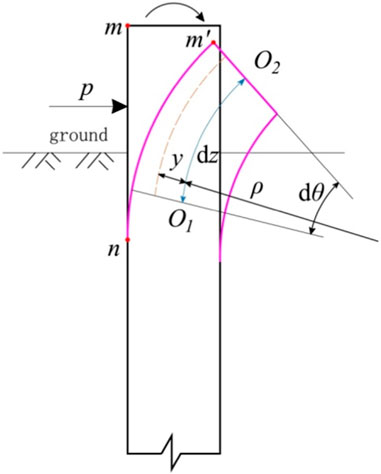
FIGURE 1. Deformation diagram of pile body under horizontal load.

Substituting Eq. 5 into Eq. 6 yields the following relationship:

${\mathit{\epsilon }}_{\mathit{m}}\left(\mathit{z}\right)=\frac{\mathit{y}\left(\mathit{z}\right)}{\mathit{\rho }\left(\mathit{z}\right)}(7)$

When the pile is bent, the relationship between the curvature radius and the bending moment is:

$\frac{\mathbf{1}}{\mathit{\rho }\left(\mathit{z}\right)}=\frac{\mathit{M}\left(\mathit{z}\right)}{\mathit{E}\mathit{I}}(8)$

In Eq. 8: $EI$ is the bending stiffness, $\mathrm{k}\mathrm{N}\cdot {\mathrm{m}}^2$; $E$ is the elastic modulus; and $I$ is the moment of inertia of the pile section.

$\mathit{M}\left(\mathit{z}\right)=\mathit{E}\mathit{I}\frac{{\mathit{\epsilon }}_{\mathit{m}}\left(\mathit{z}\right)}{\mathit{y}\left(\mathit{z}\right)}(9)$

The curvature of the plane curve can be calculated by mathematical theory:

$\frac{\mathbf{1}}{\mathit{\rho }\left(\mathit{z}\right)}=\pm \frac{{\mathit{d}}^{\mathbf{2}}\mathit{\omega }}{\mathit{d}{\mathit{z}}^{\mathbf{2}}}(10)$

Substituting Eq. 10 into Eq. 8 yields:

$\pm \frac{{\mathit{d}}^{\mathbf{2}}\mathit{\omega }}{\mathit{d}{\mathit{z}}^{\mathbf{2}}}=\frac{\mathit{M}\left(\mathit{z}\right)}{\mathit{E}\mathit{I}}(11)$

According to the sign convention between the bending moment and deflection, take the negative sign on the left side of Eq. 9, that is:

$\frac{{\mathit{d}}^{\mathbf{2}}\mathit{\omega }}{\mathit{d}{\mathit{z}}^{\mathbf{2}}}=-\frac{\mathit{M}\left(\mathit{z}\right)}{\mathit{E}\mathit{I}}=-\frac{{\mathit{\epsilon }}_{\mathit{m}}\left(\mathit{z}\right)}{\mathit{y}\left(\mathit{z}\right)}(12)$

Substituting Eq. 9, 10 into Eq. 12, an approximate solution for the torsional crankshaft is obtained. Although there is an action subjected to horizontal loads, the deformation of the pile bottom is minor enough to be negligible. Given the above reasons, it is assumed that the bottom end of the pile is completely fixed, the deflection is integrated to obtain the general solution equation of deflection:

$\mathit{w}\left(\mathit{z}\right)=-{\int }_{\mathit{H}}^{\mathit{z}}{\int }_{\mathit{H}}^{\mathit{z}}\frac{{\mathit{\epsilon }}_{\mathit{m}}\left(\mathit{z}\right)}{\mathit{y}\left(\mathit{z}\right)}\mathit{d}\mathit{z}\mathit{d}\mathit{z}-\mathit{C}\mathit{z}-\mathit{D}(13)$

In Eqs. 13, H is the burial depth of the pile; C, D is the constant of integration The discrete data can be obtained by solving:

$\mathit{w}\left(\mathit{z}\right)={\displaystyle {\sum }_{\mathit{i}=\mathbf{1}}^{\mathit{n}}}{\displaystyle {\sum }_{\mathit{i}=\mathbf{1}}^{\mathit{n}}}\frac{{\mathit{\epsilon }}_{\mathit{m}}\left({\mathit{z}}_{\mathit{i}}\right)}{\mathit{R}}∆\mathit{z}∆\mathit{z}(14)$

In Eq. 14, n is the number of measuring points from the pile bottom to the depth of z; R is the pile radius; and ∆Z is the testing distance interval of the fiber optic monitoring instruments.In Figure 1: $p$ is the horizontal load; $\rho$ is the curvature radius.

3 Introduction to HSS model

A large amount of engineering experiences indicate that it is quite difficult to accurately analyze and predict geotechnical engineering deformation. One possible important reason is the lack of reasonable understanding and application of soil deformation characteristics, especially the small strain. At present, the Hardening Soil-small (HSS) model has been widely used for deformation analysis in practical engineering due to its ability to properly consider the non-linear and stress-related characteristics of the modulus of the elastic (small strain) phase of soil. This model further optimizes the assumed conditions of the Hardening Soil (HS) model. It is an advanced soil model developed based on the fruits of soil consolidation tests and triaxial tests. The HS model simulates the shear hardening and volume hardening of soil when unloading during the plastic stage of the soil. These two hardening situations explain the stress state of internal deformation and failure of soil, which generally occur simultaneously. The results of their hardenings should be determined by the stress path and the characteristics of the soil; therefore, they can simulate various types of soil in a comparatively realistically way. The relationship between the axial strain and deviatoric stress of consolidated soil is shown in Figure 2.

FIGURE 2

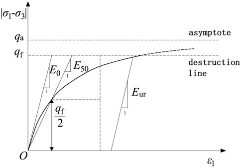
FIGURE 2. Relationship between axial strain and deviatoric stress of consolidated soil.

In Figure 2: $q_{\mathrm{a}}$ is the asymptotic value of hyperbola; $E_{50}$ is the stiffness modulus related to the confining pressure of soil; $E_{\mathrm{u}\mathrm{r}}$ is the modulus adopted by the stress path of unloading and reloading; and $E_0$ is the stiffness of soil under very small strain. $q_{\mathrm{a}}$, $E_{50}$, and $E_{\mathrm{u}\mathrm{r}}$ can be obtained from the following equation.

${\mathit{E}}_{\mathbf{50}}={\mathit{E}}_{\mathbf{50}}^{\mathit{r}\mathit{e}\mathit{f}}{\left(\frac{{\mathit{c}}^{\prime }\mathbf{cot}{\mathit{\phi }}^{\prime }-{{\mathit{\sigma }}_{\mathbf{3}}}^{\prime }}{{\mathit{c}}^{\prime }\mathbf{cot}{\mathit{\phi }}^{\prime }+{\mathit{p}}^{\mathit{r}\mathit{e}\mathit{f}}}\right)}^{\mathit{m}}(15)$

${\mathit{E}}_{\mathit{u}\mathit{r}}={\mathit{E}}_{\mathit{u}\mathit{r}}^{\mathit{r}\mathit{e}\mathit{f}}{\left(\frac{{\mathit{c}}^{\prime }\mathbf{cot}{\mathit{\phi }}^{\prime }-{{\mathit{\sigma }}_{\mathbf{3}}}^{\prime }}{{\mathit{c}}^{\prime }\mathbf{cot}{\mathit{\phi }}^{\prime }+{\mathit{p}}^{\mathit{r}\mathit{e}\mathit{f}}}\right)}^{\mathit{m}}(16)$

${\mathit{q}}_{\mathit{f}}=\left({\mathit{c}}^{\prime }\mathbf{cot}{\mathit{\phi }}^{\prime }-{{\mathit{\sigma }}_{\mathbf{3}}}^{\prime }\right)\frac{\mathbf{2}\mathbf{sin}{\mathit{\phi }}^{\prime }}{\mathbf{1}-\mathbf{sin}{\mathit{\phi }}^{\prime }}$

${\mathit{q}}_{\mathit{a}}=\frac{{\mathit{q}}_{\mathit{f}}}{{\mathit{R}}_{\mathit{f}}}(17)$

In the formula: $E_{50}^{\mathrm{r}\mathrm{e}\mathrm{f}}$ is the reference stiffness modulus; $E_{\mathrm{u}\mathrm{r}}^{\mathrm{r}\mathrm{e}\mathrm{f}}$ is the modulus of unloading and reloading; $q_{\mathrm{f}}$ is the ultimate shear stress; $R_{\mathrm{f}}$ is the damage ratio; $p^{\mathrm{r}\mathrm{e}\mathrm{f}}$ is the reference confining pressure; $c^{\prime }$ is the effective cohesion; ${\phi }^{\prime }$ is the effective internal friction angle; $m$ is the dependence index of stiffness level; and ${{\sigma }_3}^{\prime }$ is the effective small principal stress.

Based on the HS model, the HSS model takes the small strain properties of the soil into account by adding two parameters, making the simulation closer to the real situation. In dynamic triaxial tests, the small strain characteristics of soil is discovered, and the HSS model considers the increasing trend of soil stiffness under small strain conditions. Therefore, its soil excavation simulation under unloading has better adaptability compared to other constitutive models.

The empirical formula of small strain stiffness G₀^ref is:

As Hardin et al. [28] deduced through extensive experiments, the empirical formula of small strain stiffness G₀^ref is:

${\mathit{G}}_{\mathbf{0}}^{\mathit{r}\mathit{e}\mathit{f}}=\mathbf{33}\times \frac{{\left(\mathbf{2.973}-{\mathit{e}}_{\mathbf{0}}\right)}^{\mathbf{2}}}{\mathbf{1}+{\mathit{e}}_{\mathbf{0}}}{\left(\mathit{O}\mathit{C}\mathit{R}\right)}^{\mathit{m}}(18)$

In Equation 18: $e_0$ is the initial void ratio of the soil; $G_0^{\mathrm{r}\mathrm{e}\mathrm{f}}$ is the reference shear modulus for small strains; and $OCR$ is the over consolidation ratio.

According to the research of Brinkgreve and Broere. (2006), ${\gamma }_{0.7}$ can be expressed as:

${\mathit{\gamma }}_{\mathbf{0.7}}=\frac{\mathbf{1}}{\mathbf{9}{\mathit{G}}_{\mathbf{0}}}\left[\mathbf{2}{\mathit{c}}^{\prime }\left(\mathbf{1}+\mathbf{2}\mathbf{cos}\left(\mathbf{2}{\mathit{\phi }}^{\prime }\right)\right)-{{\mathit{\sigma }}_{\mathbf{1}}}^{\prime }\left(\mathbf{1}+{\mathit{K}}_{\mathbf{0}}\right)\mathbf{sin}\left(\mathbf{2}{\mathit{\phi }}^{\prime }\right)\right](19)$

For Equation 19, there exists:

${\mathit{G}}_{\mathbf{0}}={\mathit{G}}_{\mathbf{0}}^{\mathit{r}\mathit{e}\mathit{f}}\left(\frac{{\mathit{c}}^{\prime }\mathbf{cot}{\mathit{\phi }}^{\prime }-{{\mathit{\sigma }}_{\mathbf{3}}}^{\prime }}{{\mathit{c}}^{\prime }\mathbf{cot}{\mathit{\phi }}^{\prime }+{\mathit{p}}^{\mathit{r}\mathit{e}\mathit{f}}}\right)(20)$

In Equations 19, 20: ${{\sigma }_1}^{\prime }$ is the effective major principal stress; $G_0$ is the initial shear modulus under static load; $G_0^{\mathrm{r}\mathrm{e}\mathrm{f}}$ is the reference initial shear modulus for small strains; and $K_0$ is the normally consolidated lateral pressure coefficient at rest.

4 Sparrow search algorithm BP (SSA-BP) neural network model

4.1 Sparrow search algorithm principle

The Sparrow Search Algorithm (SSA) is a swarm intelligence algorithm based on the sparrow population proposed for the first time in 2020 (Xue and Shen, 2020). Its main inspiration comes from the behavior of sparrow populations in foraging and anti-predation. By optimizing the exploration and development of search space to a certain extent, SSA has a great improvement over other common intelligent optimization algorithms in search accuracy, convergence efficiency, stability, and the obviation of local optimal solution, which makes it a novel method of global search optimization.

The sparrow search algorithm consists of three different roles: producers, scroungers, and early warnings Among them, individuals with a high level of adaptability in a population are called producers, typically accounting for 10%–20% of the entire population. The rest of the individuals are scroungers, relying on the producers who find a source of food to obtain nutrition. Meanwhile, scroungers may engage in competition with producers. Any sparrow can turn into a producer by searching for better food sources. However, the total proportion of producers and scroungers in the group remains steady.

Furthermore, a certain proportion of early warmings would randomly generate in the sparrow population, usually within the range of 10%–20%. The scouters’ pivotal role is to detect potential threats such as predators, and to send alarm signals upon detection. If the alarm signal exceeds a certain safety threshold, the producers are responsible for leading all scroungers to a safe area. The position of the sparrow population is simulated by using the following matrix:

$\mathit{X}=\left[\begin{array}{c}\begin{array}{ccc}{\mathit{x}}_{\mathbf{1,1}}& {\mathit{x}}_{\mathbf{1,2}}& \dots \\ {\mathit{x}}_{\mathbf{2,1}}& {\mathit{x}}_{\mathbf{2,2}}& \dots \end{array}\begin{array}{cc}\dots & {\mathit{x}}_{\mathbf{1},\mathit{n}}\\ \dots & {\mathit{x}}_{\mathbf{2},\mathit{n}}\end{array}\\ \begin{array}{ccc}⋮& ⋮& ⋮\\ {\mathit{x}}_{\mathit{m},\mathbf{1}}& {\mathit{x}}_{\mathit{m},\mathbf{2}}& \dots \end{array}\begin{array}{cc}⋮& ⋮\\ \dots & {\mathit{x}}_{\mathit{m},\mathit{n}}\end{array}\end{array}\right](21)$

In the formula, m is the number of sparrows and N is the dimension of the variables to be optimized.

Corresponding fitness of the sparrow population:

$\mathit{F}\left(\mathit{X}\right)=\left[\begin{array}{c}\begin{array}{c}\mathit{f}\left(\left[\begin{array}{cc}{\mathit{x}}_{\mathbf{1,1}}& {\mathit{x}}_{\mathbf{1,2}}\end{array}\begin{array}{ccc}\dots & \dots & {\mathit{x}}_{\mathbf{1},\mathit{n}}\end{array}\right]\right)\\ \mathit{f}\left(\left[\begin{array}{cc}{\mathit{x}}_{\mathbf{2,1}}& {\mathit{x}}_{\mathbf{2,2}}\end{array}\begin{array}{ccc}\dots & \dots & {\mathit{x}}_{\mathbf{2},\mathit{n}}\end{array}\right]\right)\end{array}\\ ⋮\\ \mathit{f}\left(\left[\begin{array}{cc}{\mathit{x}}_{\mathit{m},\mathbf{1}}& {\mathit{x}}_{\mathit{m},\mathbf{2}}\end{array}\begin{array}{ccc}\dots & \dots & {\mathit{x}}_{\mathit{m},\mathit{n}}\end{array}\right]\right)\end{array}\right](22)$

$={\left[\begin{array}{cc}\mathit{f}\left({\mathit{x}}_{\mathbf{1}}\right)& \mathit{f}\left({\mathit{x}}_{\mathbf{2}}\right)\end{array}\begin{array}{cc}\dots & \mathit{f}\left({\mathit{x}}_{\mathit{m}}\right)\end{array}\right]}^{\mathit{T}}$

In the formula, ${\mathit{x}}_m$ is the position of the mth sparrow and $f\left({\mathit{x}}_m\right)$ is the fitness value of the mth sparrow.

The updated description of the producers’ location is as follows:

${\mathit{x}}_{\mathit{i},\mathit{j}}^{\mathit{t}+\mathbf{1}}=\left\{\begin{array}{c}{\mathit{x}}_{\mathit{i},\mathit{j}}^{\mathit{t}}.\mathit{exp}\left(\frac{-\mathit{i}}{\mathit{\alpha }\mathit{T}}\right),{\mathit{R}}_{\mathbf{2}}<\mathit{S}\mathit{T}\\ {\mathit{x}}_{\mathit{i},\mathit{j}}^{\mathit{t}}+\mathit{Q}.\mathit{L},{\mathit{R}}_{\mathbf{2}}\ge \mathit{S}\mathit{T}\end{array}\right.(23)$

In the formula: $t$ is the current number of iterations; $T$ is the maximum number of iterations; $Q$ is the random number subjected to standard normal distribution; $\mathit{L}$ is the 1 × N matrix with internal elements all being 1; $R_2$ ($R_2\in \left[\mathrm{0,1}\right]$) is the warning value of the system; and $ST$ ($ST\in \left[\mathrm{0.5,1}\right]$) is the safety value of the system.

When $R_2<ST$, it indicates that the environment is safe, that is, there are no predators around the sparrow population. In this setting, the producers are in a widespread search state. When $R_2\ge ST$, it suggests that a certain number of scouters have detected dangerous predators and sent alarm signals. At this point, the sparrow population, led by the producers, quickly makes an anti-predation response and move to another safety zone.

The updated description of the scroungers’ location is as follows:

${\mathit{x}}_{\mathit{i},\mathit{j}}^{\mathit{t}+\mathbf{1}}=\left\{\begin{array}{c}\mathit{Q}.\mathit{exp}\left(\frac{{\mathit{x}}_{\mathit{w}}^{\mathit{t}}-{\mathit{x}}_{\mathit{i},\mathit{j}}^{\mathit{t}}}{{\mathit{i}}^{\mathbf{2}}}\right),\mathit{i}>\frac{\mathit{n}}{\mathbf{2}}\\ {\mathit{x}}_{\mathit{p}}^{\mathit{t}+\mathbf{1}}+\left|{\mathit{x}}_{\mathit{i},\mathit{j}}^{\mathit{t}}-{\mathit{x}}_{\mathit{p}}^{\mathit{t}+\mathbf{1}}\right|.{\mathit{A}}^{+}.\mathit{L},\mathit{i}\le \frac{\mathit{n}}{\mathbf{2}}\end{array}\right.(24)$

In the formula, $x_{\mathrm{p}}^t$ is the optimal position occupied by the current producers; $x_{\mathrm{w}}^t$ is the current global worst position; and ${\mathit{A}}^{+}$ is the 1 × n matrix, with randomly distributed elements of one or -1 which satisfies ${\mathit{A}}^{+}={\mathit{A}}^{\mathrm{T}}{\left(\mathit{A}{\mathit{A}}^{\mathrm{T}}\right)}^{-1}$.

The updated description of the early warmings’ location is as follows:

${\mathit{x}}_{\mathit{i},\mathit{j}}^{\mathit{t}+\mathbf{1}}=\left\{\begin{array}{c}{\mathit{x}}_{\mathit{b}}^{\mathit{t}}+\mathit{\beta }.\left|{\mathit{x}}_{\mathit{i},\mathit{j}}^{\mathit{t}}-{\mathit{x}}_{\mathit{b}}^{\mathit{t}}\right|,{\mathit{f}}_{\mathit{i}}\ne {\mathit{f}}_{\mathit{g}}\\ {\mathit{x}}_{\mathit{i},\mathit{j}}^{\mathit{t}}+\mathit{K}.\left(\frac{\left|{\mathit{x}}_{\mathit{i},\mathit{j}}^{\mathit{t}}-{\mathit{x}}_{\mathit{w}}^{\mathit{t}}\right|}{\left({\mathit{f}}_{\mathit{i}}-{\mathit{f}}_{\mathit{w}}\right)+\mathit{\epsilon }}\right),{\mathit{f}}_{\mathit{i}}={\mathit{f}}_{\mathit{g}}\end{array}\right.(25)$

In the equation: $x_{\mathrm{b}}^t$ is the current location that coincides with the center of gravity of the species group, which refers to the current global optimal position; $\beta$ is the step size control parameters, obeying the normal distribution with a mean value of 0 and variance of 1; $K$ is a uniformly distributed random variable on the interval [-1,1]; $f_{\mathrm{g}}$ and $f_{\mathrm{w}}$ are, respectively, the current fitness values under the global optimal and worst conditions; $f_i$ is the fitness value corresponding to the ith sparrow in the current iteration; and $\epsilon$ is the arbitrarily small number, which satisfies the condition of meaningful fractions.

When $f_i\ne f_{\mathrm{g}}$, it means that the sparrows are at the edge of the group and easier to recognize the danger; therefore, they need to be ready to change the position at any time to achieve a higher fitness. When $f_i=f_{\mathrm{g}}$ , it denotes that the center of the population have also perceived the danger, which requires a quick approach from other individuals to avoid predators.

4.2 SSA-BP model

The performance of the BP neural network depends on the setting of its weights and thresholds; for this reason, optimizing these parameters is necessary to improve the performance. In the traditional optimization methods, problems such as non-convexity, high dimensionality, and multimodality often need to be tackled with, and the computational complexity is very high and prone to falling into local optimal solutions. As a new type of heuristic optimization algorithm, the sparrow search algorithm can avoid these problems. It can search for the optimal solution by imitating the sparrow’s foraging behavior and the global optimal solution in a short time with high efficiency and accuracy.

In accordance with the improved algorithms above, employing the sparrow search algorithm to optimize the weights and thresholds of the BP neural network can enhance its accuracy and generalization ability, so as to better adapt to practical application scenarios. Additionally, this method has a good optimization effect in preventing some of the problems of traditional optimization methods, such as local optimal solutions and high computational complexity. Therefore, the sparrow search algorithm is an optimization method suitable for the BP neural network. The prediction flow chart of the improved SSA-BP model is shown in the following Figure 3:

FIGURE 3

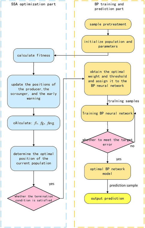
FIGURE 3. Prediction flow chart of SSA-BP model.

5 Introduction to deep foundation pit engineering

5.1 Introduction of the engineering

The deep foundation pit engineering in Dalian Donggang Business District, with a length of about 100 m and a width of about 50 m, is equipped with a three story basement. The depth of the foundation pit is 14.0–15.7 m, its excavating area being about 5,150 m². The plan of using a secant pile with two reinforced concrete internal supports has been adopted as the foundation pit support structure. The design of the brace layout is that the north side adopts the ring brace while the south side takes the corner brace. In addition, the support pile put to use is a 1.2 m diameter secant pile. The cross-section of the foundation pit support system is illustrated in Figure 4.

FIGURE 4

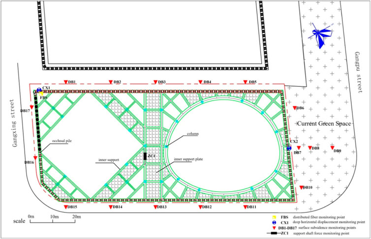
FIGURE 4. Layout plan and measurement points of the foundation pit.

The strata on the site of this project are in sequence from top to bottom: plain fill, mucky silty clay, silty clay, completely weathered slate, intensely weathered slate, moderately weathered slate, and slightly weathered slate. In terms of the engineering example of the adjacent parallel field, the water level elevation of groundwater in the surrounding area of the site reaches 1.80 m. Its main aquifer is earth fill, which is a strong permeable stratum.

5.2 Layout of conventional deep foundation pit monitoring

In order to ensure the stability and safety of the foundation pit engineering, impactful monitoring must be carried out throughout the construction. To analyze the results of monitoring, it is necessary to conduct global monitoring, comprehensively analyzing multiple associated measurement points and monitoring projects. By doing so, it is beneficial to reduce construction risks by determining whether the support design is in need of modification, and whether there is room for improvement in the construction technology and methods. It is also conducive to monitor the deformation and safety of the surrounding construction areas. Figure 4 shows the layout plan and measurement points of the foundation pit.

The stratigraphic distribution and characteristics of the site of this project are as follows, and the typical engineering geological sectional drawing is shown in Figure 5.

FIGURE 5

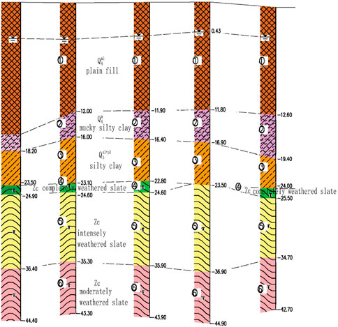
FIGURE 5. Typical engineering geological sectional drawing of the foundation pit.

Plain fill: in a slightly dense state, mainly composed of cohesive soil, slate, and quartzite gravels. The particle grading is ordinary, with an average Cone dynamic penetration test (DPT) of 6.2.

Mucky silty clay: in a soft plastic state, with a high content of organic matter.

Silty clay: in a plastic state, locally containing quartz fine sand, with an average standard penetration test (SPT) of 9.8.

Completely weathered slate: extremely soft rock and terribly fractured.

Intensely weathered slate: with developed joints and fissures, soft rock, and fractured. The basic quality level of the rock mass is Grade V.

Moderately weathered slate: the rock core is in a block and short column shape, with developed joints and fissures. The rock mass is of a layered structure and relatively complete. Its basic quality grade is Grade IV.

Slightly weathered slate: relatively hard rock; the basic quality level of the rock mass is Grade III.

Figure 6 manifests the sectional drawing of the foundation pit support system, which is located in the upper left side of the layout plan. According to the requirements of relevant specifications, combined with the support design of the foundation pit engineering as well as the actual construction situation onsite, the monitoring objects of the project were determined to include the foundation pit support structure and surface settlement outside the pit, etc. The content and items of routine monitoring are as follows:

(1) Horizontal deformation of the support pile (CX1-CX7).

(2) Ground surface settlement monitoring (DB1-DB17).

FIGURE 6

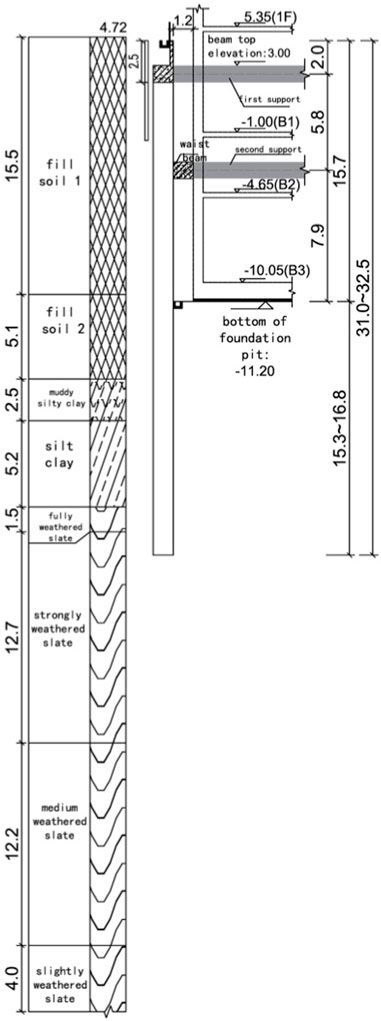
FIGURE 6. Sectional drawing of the foundation it support system.

In line with the specifications and design requirements, the horizontal displacement was monitored by using an inclinometer. According to the design documents for the foundation pit support of this project, it was planned to set up seven deep horizontal displacement points. They were respectively arranged at the corners of the support structure and in the middle of the long side, with a horizontal spacing of no more than 50 m between two monitoring points. The point numbers above are: CX1∼CX7.

The monitoring points of the ground surface settlement around the foundation pit were set on the sidewalks and green belts surrounding the pit. Of them, there were two additional points added to the original green space on the north side. The point numbers above are: DB1∼DB17.

5.3 Layout of distributed optical fiber monitoring

In view of the harsh construction environment such as soil filling and grouting, the research team applied tightly sleeved optical fiber technology in this monitoring study. It has the favorable form of encapsulation protection and fine effect of strain transmission; hence, it can adapt to the harsh working environment of the underground diaphragm wall. The technology breaks through the traditional concept of point sensing to measure strain, temperature, and damage information at any point on the optical fiber, execute continuous distributed monitoring of the measured objects, and study the overall strain behavior of the measured objects, in order to achieve the purpose of guiding the site construction and later structural health diagnosis.

This project used the distributed optical fiber method to monitor the southwest section of the foundation pit. The support pile adopted is a 1.2 m diameter secant pile, and the length of the pile in this section is 32 m according to the design drawing of the foundation pit support. The experimental system is shown in Figure 7. Depending on different types of pile, considering the survival rate of sensing fibers, operability of construction, and installation, as well as monitoring accuracy, it is required to handle crucial technical aspects including the layout plan and temperature compensation. There were at least four sensing optical cables that needed to be set inside the cast-in-place pile, and the optical fibers were laid on the main reinforcement of the steel cage by using rebar as the carrier. Additionally, the optical fibers needed to be laid along the inner side of the rebars to prevent the direct impact of concrete on the optical fibers during concrete pouring. In order to systematically grasp the real situation of the pile, a dual U-shaped method was adopted to ensure the survival rate of the optical fiber and the reliability of the data.

FIGURE 7

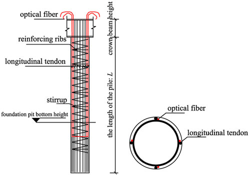
FIGURE 7. Schematic diagram of field test of deep foundation pit support structure.

After rebar workers on the construction site finished the steel cage, the main reinforcement position where the optical fiber was to be pasted needed to be ground and then wiped clean with alcohol wipes. Next, tightly sleeved optical fibers at the corresponding positions of rebars were laid before 502 glue was evenly applied. When pasting distributed optical fibers, attention needed to be paid to straightening the fibers and sticking them without relaxation. The bend needed to be protected by a metal hose—this part of the dataset was not studied. After that, the steel pipe was used to connect the optical fiber at the pile head, and coil the fibers to prevent damage caused by the hoisting of the steel cage.

Metal-based cord-like optical fibers have good encapsulation technology, and the strain transmission effect is within a controllable range. Therefore, they were arranged along the main reinforcement of the steel cage symmetrically and placed on the inner side of the steel cage, where it was difficult to touch the surrounding rock and soil as well as the grouting equipment. A dedicated locking device and epoxy were used to tighten when fixing the optical fiber at fixed intervals, which prevented them from slipping. The sensing optical cable was pre-tensioned to keep itself straight, and was fixed using the binding method. Large intervals could be taken when binding the temperature compensated optical fibers. The onsite operation of the optical fiber monitoring scheme is demonstrated in Figure 8.

FIGURE 8

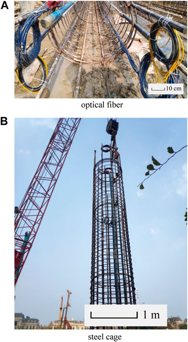
FIGURE 8. Photos of the onsite operation of the optical fiber monitoring scheme. (A) optical fiber. (B) steel cage.

The temperature sensing compensation optical fibers are tightly sleeved optical fibers and was installed parallel to the measurement object. Furthermore, the indirect compensation method was used to install a temperature compensation optical cable which is not affected by the structural strain beside the sensing optical cable. The real strain of the measurement object was obtained by subtracting the measured value of the temperature compensation optical cable from the monitoring result of the deformation monitoring optical cable.

5.4 Monitoring instruments

The optical fiber data acquisition device utilized in this research is the Neubrex NBX-8100 from Japan. Table 1 shows the parameters of the NBX-8100, which uses PSP-BOTDR technology. This equipment went into production in 2018, and it is the most advanced product in the field of distributed optical fiber in the international industry. It has the smallest spatial resolution and the most stable performance, and all of its indicators fulfill the requirements of this experiment. The exterior of the instrument is shown in Figure 9.

TABLE 1

TABLE 1. Optical nanometer parameter settings.

FIGURE 9

FIGURE 9. NBX-8100 optical nanometer.

The sensing optical cable adopts the metal-based cord-like strain sensing optical cables (model: NZS-DSS-C02) produced by Suzhou Nanzhi Sensing Technology Co., Ltd. This sensing optical cable is protected by multiple metal reinforcements. Used in conjunction with Brillouin Optical Time Domain Reflectometry (BOTDR), the surface strength has been greatly improved and the measurement results can be directly used in displacement conversion providing technical support for test results. The research group (Wang G. et al., 2020) has calibrated the sensing optical cable in the early stage to obtain the temperature and strain coefficients of the cable. The performance and technical parameters of the sensing optical cable are shown in Table 2.

TABLE 2

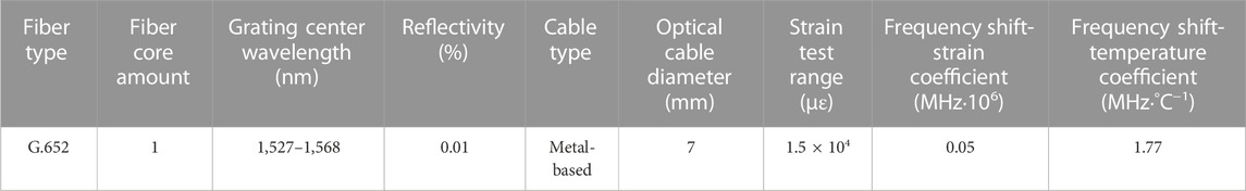
TABLE 2. Performance and technical parameters of the optical fiber sensor.

6 Back-analysis of HSS model parameters

6.1 Finite element analysis

Using Plaxis for numerical analysis and calculation, a two-dimensional finite element model of the northern ring brace section (section 1-1) of the foundation pit was established. The excavation length of the model was 100 m, the excavation depth was 14 m, and the length of the secant pile was 32 m. The complexity of the calculation was reduced by using a half structure. The excavation size inside the pit was 29.7 m, the ground behind the secant pile was 76 m, and the model’s vertical dimension was around 60 m. Both the road load and the construction load around the foundation pit were assumed to be 15 kPa. Although the model’s ultimate size was 100 m × 60 m, to simplify the model and make calculation easier, the local pile grid and load grid were encrypted during the grid generation procedure. The final northern ring brace model was divided into 2,596 units including 21,303 nodes. The boundary conditions were lower full constraint, left and right normal constraint, and top free constraint. The final grid generation result is shown in Figure 10.In accordance with the previous research results of many scholars, a conservative method was adopted. The secant pile was transformed into a diaphragm wall and simulated by using plate elements based on the principle of equivalent stiffness. Calculation of the moment of inertia was based on the structural diagram of the secant pile in Figure 11:

FIGURE 10

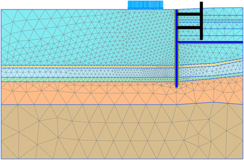
FIGURE 10. Mesh division of deep foundation pit model in section one to one.

FIGURE 11

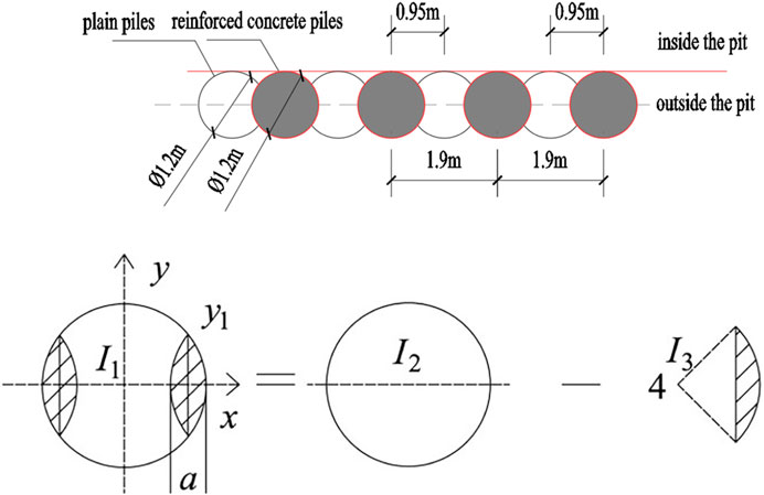
FIGURE 11. Structural diagram and moment of inertia calculation diagram of the secant pile.

In Formulas 21, 22, and 23, I₁ is the moment of inertia of a single pile minus the black part in the figure; I₂ is the cross-sectional moment of inertia of the common pile; I₃ is the moment of inertia of the quarter black part of the secant pile; R is the radius of the pile; a is the secant distance between two piles; and y₁ is half of the width of the secant face surface.

Calculation of the equivalent thickness $h_0$ was based on the principle of equivalent stiffness:

${\mathit{I}}_{\mathbf{1}}={\mathit{I}}_{\mathbf{2}}-\mathbf{4}{\mathit{I}}_{\mathbf{3}},(26)$

${\mathit{I}}_{\mathbf{2}}=\frac{\mathbf{1}}{\mathbf{4}}\mathit{\pi }{\mathit{R}}^{\mathbf{4}},(27)$

${\mathit{I}}_{\mathbf{3}}={\displaystyle {\int }_{{-\mathit{y}}_{\mathbf{1}}}^{{\mathit{y}}_{\mathbf{1}}}}{\mathit{y}}^{\mathbf{2}}\left[\mathit{x}-\left(\mathit{R}-\frac{\mathit{a}}{\mathbf{2}}\right)\right]\mathit{d}\mathit{y}=\mathbf{2}{\displaystyle {\int }_{\mathbf{0}}^{{\mathit{y}}_{\mathbf{1}}}}{\mathit{y}}^{\mathbf{2}}\sqrt{{\mathit{R}}^{\mathbf{2}}-{\mathit{y}}^{\mathbf{2}}}\mathit{d}\mathit{y}=\sqrt{{\mathit{R}}^{\mathbf{2}}-{{\mathit{y}}_{\mathbf{1}}}^{\mathbf{2}}}\frac{\left({\mathit{R}}^{\mathbf{2}}-\mathbf{2}{{\mathit{y}}_{\mathbf{1}}}^{\mathbf{2}}\right)}{\mathbf{4}}-\frac{\left(\mathbf{2}\mathit{R}-\mathit{a}\right){{\mathit{y}}_{\mathbf{1}}}^{\mathbf{3}}}{\mathbf{3}}(28)$

${{\mathit{E}}_{\mathbf{1}}\mathit{I}}_{\mathbf{1}}+{{\mathit{E}}_{\mathbf{2}}\mathit{I}}_{\mathbf{2}}=\frac{{\mathit{E}}_{\mathbf{0}}\left(\mathbf{4}\mathit{R}-\mathbf{2}\mathit{a}\right){{\mathit{h}}_{\mathbf{0}}}^{\mathbf{3}}}{\mathbf{12}}(29)$

${\mathit{E}}_{\mathbf{0}}=\frac{{{\mathit{E}}_{\mathbf{1}}\mathit{A}}_{\mathbf{1}}+{{\mathit{E}}_{\mathbf{2}}\mathit{A}}_{\mathbf{2}}}{\left({\mathit{A}}_{\mathbf{1}}+{\mathit{A}}_{\mathbf{2}}\right)}(30)$

In the formula, E1 is the elastic modulus of plain piles, E2 is the elastic modulus of reinforced piles; E0 is the equivalent elastic modulus; A1 is the cross-sectional areas of plain piles, A2 is the cross-sectional areas of reinforced piles; and h0 is the equivalent thickness.

The support is composed of C40 concrete, the reinforced piles are made of C30 concrete, and the plain piles are made of C15 concrete. The input parameters for the inner support, which is simplified by using anchor rods for simulation, are shown in Table 3. The simulation parameters following the equivalent calculation of the secant pile are shown in Table 4.

TABLE 3

TABLE 3. Support numerical simulation parameters.

TABLE 4

TABLE 4. Numerical simulation parameters of the plate element.

Before beginning the calculation, the calculation phase must be defined Because of the non-uniformity of the foundation soil layer, the calculation method of gravity loading was employed to construct the initial stress field in the initial stage. The water level is set and the phreatic water type is selected as the pore pressure calculation type. At the initial stage, only the soil element is active, while the other structural elements and road loads are deactivated. Before excavation, the plate unit and road load are activated, and the displacement of the obtained data reset to zero.

Pore pressure, having some significant impact on the deformation of foundation pits, should be taken into account. In the actual engineering of this paper, thanks to the sound sealing performance of the secant pile, the calculation method of stable seepage was used to consider the changes in pore pressure caused by foundation pit excavation. The seepage computation of the model was not considered due to the secant pile’s superior waterstop capability The specific excavation sequence of the foundation pit is shown in Table 5.

TABLE 5

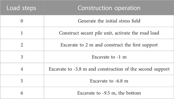
TABLE 5. Sequence of excavation of The deep foundation pit.

6.2 Sensitivity analysis of parameters

The HSS model comprises many parameters, and sensitivity analysis of parameters is essential to improve the efficiency and accuracy of inversion analysis. In this procedure, it is vital to establish which parameters have the largest influence on the model’s output outcomes in order to optimize parameters and increase the accuracy and robustness of model prediction. Based on similar projects and relevant literature, the initial parameters of the typical soil layer HSS model in the Dalian Donggang Business District could be determined. Through a comprehensive analysis of the actual engineering values in the Yangtze River Delta region (Yin, 2010; Wang et al., 2012; Wang et al., 2013; Liang et al., 2017; Zong and Xu, 2019; Gu et al., 2021), Xiamen region (Shi et al., 2016), Tianjin region (Liu et al., 2007), and Jinan region (Li et al., 2019), it could be determined that the unloading and reloading Poisson’s ratio ${\nu }_{ur}$ is 0.20, the reference stress $p^{\mathrm{r}\mathrm{e}\mathrm{f}}$ is 100kPa, the failure ratio $R_{\mathrm{f}}$ is 0.7–0.9, the power exponent $m$ is 0.7–0.9, the reference secant modulus $E_{50}^{\mathrm{r}\mathrm{e}\mathrm{f}}\approx Es$, and the reference tangent modulus $E_{\mathrm{o}\mathrm{e}\mathrm{d}}^{\mathrm{r}\mathrm{e}\mathrm{f}}\approx Es$. Table 6 displays the HSS model’s initial parameters. As demonstrated in Table 7, this article provides both the Mohr Coulomb (M-C) constitutive model parameters for moderately weathered and slightly weathered slate.

TABLE 6

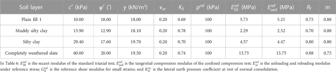
TABLE 6. Computing parameters of the HS-Small model for soil layers.

TABLE 7

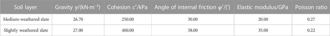
TABLE 7. Computing parameters of the MC model for soil layers.

In this sensitivity analysis, seven parameters including $E_{50}^{\mathrm{r}\mathrm{e}\mathrm{f}}$, $E_{\mathrm{o}\mathrm{e}\mathrm{d}}^{\mathrm{r}\mathrm{e}\mathrm{f}}$, $E_{\mathrm{u}\mathrm{r}}^{\mathrm{r}\mathrm{e}\mathrm{f}}$, R_f, $G_0^{\mathrm{r}\mathrm{e}\mathrm{f}}$, m, and ${\gamma }_{0.7}$ were selected as candidates, and four different types of soil layers were selected, namely plain fill, mucky silty clay, silty clay, and completely weathered slate. By observing the changing amplitude of deep horizontal displacement at the bottom of the foundation pit enclosure structure under the fluctuation of ±10% of the above seven parameters, the sensitivity of foundation pit deformation to each of the seven parameters could be assessed. Figure 11 and Figure 12 show the relative change of deep horizontal displacement when the parameter increases and decreases by 10%.

FIGURE 12

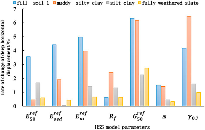
FIGURE 12. Relative displacement changes when the parameter increases by 10%.

The results of Figure 12 and Figure 13 reflect the sensitivity of the foundation pit deformation to the seven parameters, represented by the deep horizontal displacement of the support structure at the bottom of the pit. The vertical axis shows the rate of change of foundation pit deformation, which refers to the change of the new foundation pit deformation after the parameter increases or decreases by 10%. It can reflect the comparison and reference situation between the new state and the original state.

FIGURE 13

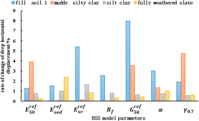
FIGURE 13. Relative displacement change when the parameter is reduced by 10%.

Figure 14 comprehensively considers the results of Figure 12 and Figure 13. The vertical axis data represent the average relative displacement when four different parameters change, and it can be seen from this that the changes of $G_0^{\mathrm{r}\mathrm{e}\mathrm{f}}$, ${\gamma }_{0.7}$, and $E_{\mathrm{u}\mathrm{r}}^{\mathrm{r}\mathrm{e}\mathrm{f}}$ had a significant impact on the calculation results. The sensitivity ranking of the seven parameters selected above were: $G_0^{\mathrm{r}\mathrm{e}\mathrm{f}}$ > ${\gamma }_{0.7}$ > $E_{\mathrm{u}\mathrm{r}}^{\mathrm{r}\mathrm{e}\mathrm{f}}$ > $E_{50}^{\mathrm{r}\mathrm{e}\mathrm{f}}$ > $E_{\mathrm{o}\mathrm{e}\mathrm{d}}^{\mathrm{r}\mathrm{e}\mathrm{f}}$ > $m$ > $R_{\mathrm{f}}$, referring to relevant literature (Shi et al., 2017; Chen et al., 2021; Gu et al., 2021; Luo et al., 2021). It can be seen that changes in small strain parameters $G_0^{\mathrm{r}\mathrm{e}\mathrm{f}}$ and ${\gamma }_{0.7}$ had a significant impact on the deformation of the foundation pit, which is in good agreement with the sensitivity analysis results in this article. Therefore, in order to guarantee the hiberarchy of the numerical simulation results, the first three parameters $G_0^{\mathrm{r}\mathrm{e}\mathrm{f}}$, ${\gamma }_{0.7}$, and $E_{\mathrm{u}\mathrm{r}}^{\mathrm{r}\mathrm{e}\mathrm{f}}$ were selected for inversion analysis.

FIGURE 14

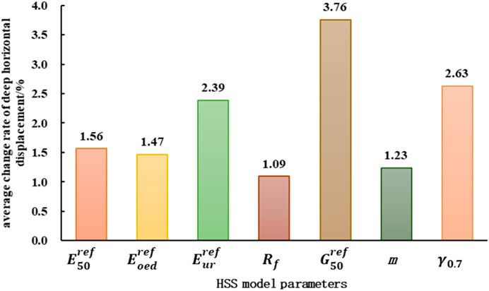
FIGURE 14. Mean value of relative displacement change in deep horizontal displacement.

6.3 Back-analysis model

6.3.1 BP neural network

On the basis of the preprocessing of raw data, MATLAB was selected as the main mathematical tool for this inversion experiment of parameters; the first 77 sets of total data samples were used as the training set to train the network model, and the last four sets were used as the test set to input the trained model for calculation. Considering the balance between data volume and model complexity, an appropriate displacement index needed to be selected which could avoid data redundancy and model overfitting and improve the generalization ability and prediction accuracy of the model. At the same time, selecting appropriate input variables can reduce the complexity of the network structure and reduce computational costs and training difficulty. In addition, in underground engineering, different displacement indicators can reflect different characteristics of deformation. For example, the uplift of the pit bottom mainly reflects the compression deformation of the underground soil layer; the ground surface settlement mainly reflects the settlement deformation of the soil layer; and the deep horizontal displacement of the soldier pile reflects the stress state changes of the surrounding soil. Taking these displacement indicators into account can more comprehensively and accurately reflect the deformation situation of underground engineering.

In summary, as per the results of the numerical simulation orthogonal experiment, a total of eight displacement indicators, including the maximum uplift of the pit bottom, three ground surface settlements (2 m outside the pit, 6 m outside the pit, and 10 m outside the pit), and four deep horizontal displacements (at the top of the pile, at support 1, at support 2, and at the bottom of the pit) of soldier piles, were selected for this back-analysis experiment. These eight indicators were used as input values for the network structure, and 12 parameters to be inverted were used as output values; thus, the input layer of the neural network included eight nodes and the output layer included 12 nodes. Through model debugging and multiple rounds of training based on reference empirical formulas, the optimal value for the number of nodes in the hidden layer was determined to be five, thereby achieving the highest accuracy of the model. Therefore, a back propagation neural network model with an 8-5-12 network structure was established. The relative error of the final result is shown in Figure 15.

FIGURE 15

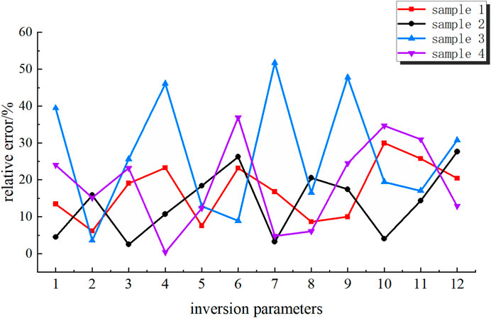
FIGURE 15. Relative error of the BP neural network test set.

The largest error among the four groups of samples was 51.7%, the minimum error was 0.3%, and the average error was 19.6%, as shown in Figure 14. To minimize the prediction error of the BP neural network as much as feasible, study on its optimization strategy was required, so an improved sparrow search algorithm was introduced to optimize it.

6.3.2 SSA-BP model

This portion continued to use the BP neural network structure of 8-5-12 from the previous section with the number of sparrows set to five and the maximum number of iterations set to 50. The network model was trained with the first 77 sets of total data samples as the training set, and then the last four sets of samples were used in the learned model for calculation. The relative error of the final results is shown in Figure 16.

FIGURE 16

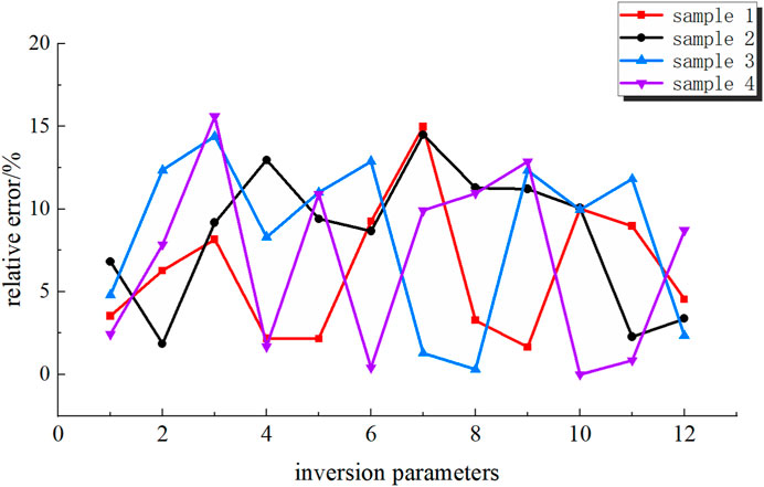
FIGURE 16. Relative error of the improved SSA-BP neural network test set.

The above graph depicts the prediction error of the BP neural network optimized by the improved sparrow search algorithm. It is easy to see that its overall trend is significantly lower than the initial BP network; the maximum error among the four groups of samples was 15.6%, the minimum error was 0.03%, and the average error was 7.51%. By analyzing the errors, it is possible to conclude that the accuracy of the optimized neural network meets the actual engineering requirements. In this paper, an improved SSA-BP neural network model was used to perform back-analysis experiments on the parameters of the HSS constitutive model, and the values of the back-analysis results are shown in Table 8.

TABLE 8

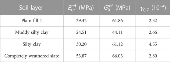
TABLE 8. Inversion analysis results table of soil parameters.

7 Result analysis

7.1 Analysis of HSS model parameter errors

After substituting the parameters in the table into the calculation of the PLAXIS finite element model, the deformation of the foundation pit was obtained. Compared with the measured data, as shown in Table 9, the maximum error between the measured value and simulated value of Section 1-1 was 8.12%, which occurred at the pile top; the minimum error was 0.53%; the average relative error was 10.43%, which is within the allowable range of error, so this parameter inversion analysis met the accuracy and precision requirements of the small strain model for simulating the excavation of foundation pits.

TABLE 9

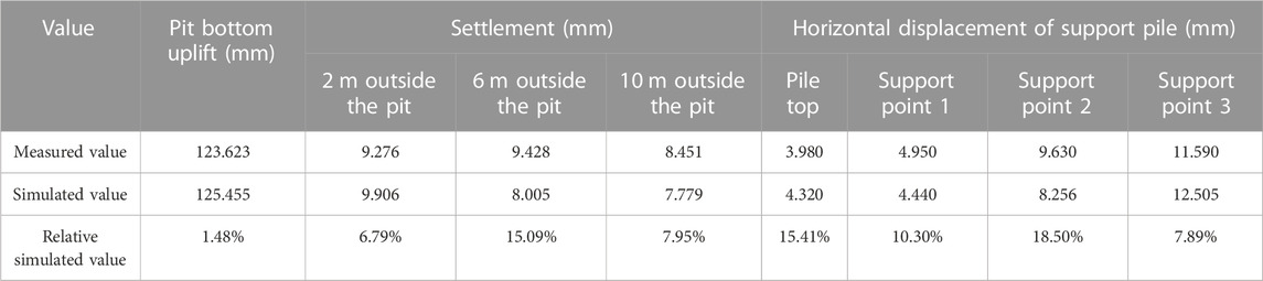
TABLE 9. Relative error between the measured value and the simulated value of the foundation pit deformation of Section 1-1.

7.2 Analysis of deep horizontal displacement

Figure 17 shows the strain monitoring data on the internal and external side of the foundation pit. The left side shows the internal optical fiber and the right side shows the external optical fiber; the pile undergoes deformation under lateral earth pressure, resulting in tensile strains on the internal sides of the foundation pit, and compressive strains on the external sides of the foundation pit.

FIGURE 17

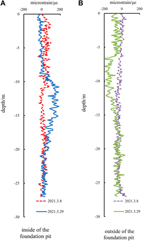
FIGURE 17. Monitoring value of the internal and external strain of the foundation pit. (A) inside of the foundation pit. (B) outside of the foundation pit.

On 8 March 2021, the inner support had not been poured and the support pile was under soil pressure on the external sides of the foundation pit, causing tensile strain on the optical fiber on the outer pile and compressive strain on the inner pile. On 29 March 2021, the pouring of first inner support was completed, and the foundation pit was excavated for the second time; near the excavation face, due to the bearing of partial soil pressure by the inner support, the support pile began to protrude and deform, causing compressive strain on the external side of the pile and tensile strain on the internal side. The monitoring results indicated that as the foundation pit is excavated, the supports of internal and external stress in the foundation pit are reversed; the inner support plays a significant role in sharing the stress of the support pile. The soil pressure load it bears continues to increase, but its axial force remains within a safe range, indicating that the inner support structure has relatively high safety.

According to the monitoring results at different stages, the lateral displacement of the support structure could be calculated by using the deflection calculation method in Section 1, as shown in Figure 18. The conventional measure in Figure 18 was to measure the deep horizontal displacement of the support pile using inclinometer; the monitoring location was located at CX1 in Figure 4. When the foundation pit was excavated to −9.5 m, the maximum measured value of the deep horizontal displacement clinometer of the support pile was 13.16 mm obtained at −10.78 m; the maximum measured value of distributed optical fiber was 11.32 mm obtained at −12.53 m; and the maximum calculated value was 16.88 mm obtained at −13.03 m. It can be concluded that the changing trends of the three are roughly the same, with the onsite optical fiber results being slightly smaller than the results of the numerical analysis; the reason for the error may be that the finite element simulation did not fully simulate the complex working conditions on site, such as construction machinery and onsite loading. The optical fiber was damaged because of onsite mechanical excavation and human factors, but there were many remaining optical fiber monitoring data samples. Because the sampling interval of the optical fiber is 0.05 m, it has a significant advantage in studying the overall performance of the measured object and can be fully compared with the results of finite element analysis.

FIGURE 18

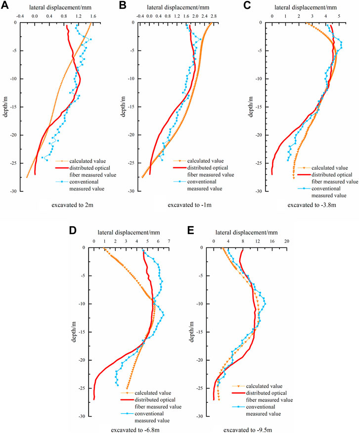
FIGURE 18. Horizontal displacement of the deep layers in section one to one. (A) excavated to 2 m. (B) excavated to −1 m. (C) excavated to −3.8 m. (D) excavated to −6.8 m. (E) excavated to −9.5 m.

The optical fiber monitoring data was close to the monitoring data of the clinometer; the sampling interval of the clinometer data is 0.5 m, which is ten times that of optical fiber monitoring. The distributed optical fiber basically realizes the structural deformation characteristics of the measured object within a very small range, making it easy to study the subtle changes in the impact of external loads, construction machinery, and other factors on the foundation pit support structure and explore their deformations. However, optical fibers require good packaging technology and laying methods to achieve precise monitoring.

7.3 Analysis of surrounding ground surface settlement

According to the monitoring of the measured points in DB7-DB9, the relationship between the ground surface settlement of the foundation pit and the distance between the measurement points and the pit edge in Figure 19 was obtained. As shown in the figure, the changing trend of measured data of settlement and simulated calculation results was basically consistent, indicating that the HSS constitutive model can well predict the ground surface settlement law around deep foundation pit. During the excavation of the foundation pit, the center of the ground surface settlement gradually moved outward; when the excavation was completed, the deformation finally stabilized. The final measured maximum value was 14.89 mm, which was obtained at a distance of 10 m from the pit edge; the simulated maximum value was −16.2, which was obtained at a distance of 12 m from the pit edge; the ratio of ground surface settlement to excavation depth of the pit was 0.157% and 0.17%, respectively.

FIGURE 19

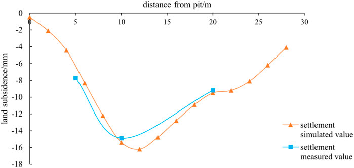
FIGURE 19. Surrounding surface subsidence.

8 Conclusion

Real-time monitoring of the full excavation deformation process of deep foundation pits was carried out for a deep foundation pit project with internal support in the Dalian Donggang Business District using a combination of traditional monitoring and distributed optical fiber monitoring. To undertake a back-analytical study of the HSS model parameters, the sparrow search algorithm was integrated with the BP neural network. Then, using the geotechnical finite element analysis software Plaxis to simulate the entire foundation pit construction process, a finite element numerical analysis model of the foundation pit was established. The main research conclusions from the comparative analysis of measured data and simulation results are as follows:

(1) With a maximum prediction error of 15.6%, a minimum prediction error of 0.03%, and an average error rate of 7.51%, the SSA-BP neural network utilized in this article performed better. The performance to predict the dataset is enhanced.

(2) The study’s back-analysis of parameters met the accuracy and precision requirements of the HSS small strain model for modeling foundation pit excavation, and can serve as a reference for comparable actual projects.

(3) The displacement values can be calculated using the micro strain values of deep horizontal displacement obtained by the NBX-8100 optical and the deflection calculation method. The data of optical fiber monitoring was similar to that of the clinometer, and the sampling interval of the optical fiber monitoring data was approximately 1/10 of the inclinometer, achieving the structural deformation characteristics of the tested object within a very small range. Furthermore, the data curve was relatively smooth and with high continuity, demonstrating the superiority of distributed optical fiber monitoring in terms of space and accuracy.

(4) The HSS constitutive model can accurately forecast horizontal deformation and surrounding surface settlement produced by deep excavation, providing the technical assistance required for stress and deformation analysis in complex excavation projects.

Data availability statement

The original contributions presented in the study are included in the article/Supplementary Material, further inquiries can be directed to the corresponding author.

Author contributions

Corresponding author JZ planned and organized the entire research and was responsible for onsite monitoring. The first author, WL, was responsible for the numerical analysis calculation and neural network analysis. YP participated in onsite monitoring work and some numerical calculations. All authors contributed to the article and approved the submitted version.

Conflict of interest

The authors declare that the research was conducted in the absence of any commercial or financial relationships that could be construed as a potential conflict of interest.

Publisher’s note

All claims expressed in this article are solely those of the authors and do not necessarily represent those of their affiliated organizations, or those of the publisher, the editors and the reviewers. Any product that may be evaluated in this article, or claim that may be made by its manufacturer, is not guaranteed or endorsed by the publisher.

Supplementary material

The Supplementary Material for this article can be found online at: https://www.frontiersin.org/articles/10.3389/fmats.2023.1231303/full#supplementary-material

References

Atkinson, J. H., and Sallfors, G. (1991). “Experimental determination of stress-strain-time characteristics in laboratory and in situ tests,” in Proceedings of the International Conference on Soil Mechanics and Foundation Engineering, Rotterdam: A.A. Balkema, 915–956.

Google Scholar

Benz, T. (2007). Small-strain stiffness of soils and its numerical consequences. Ph.D. Germany. Stuttgart: University.

Google Scholar

Brinkgreve, R. B. J., and Broere, W. (2006). Plaxis material models manual. Netherlands: Bentley Systems.

Google Scholar

Chen, Y., Luo, M., and Xia, N. (2021). Statistical analysis of existing test results of HSS model parameters for soft soils[J]. Chin. J. Geotechnical Eng. 43 (S2), 197–201.

Google Scholar

Fu, L., and Peng, Y. (2018). Development and application of safety monitoring and early warning platform for deep foundation pit. Chin. J. Undergr. Space Eng. 14 (S1), 423–429.

Google Scholar

Gao, L., Gong, Y., and Yu, Y. (2017). Development and application of distributed measurement optical fiber inclinometer tube based on Brillouin optical time-domain reflectometer. Sci. Technol. Eng. 17 (30), 81–85.

Google Scholar

Gu, X., Wu, R., and Liang, F. (2021). On HSS model parameters for Shanghai soils with engineering verification. Rock Soil Mech. 42 (03), 833–845. doi:10.16285/j.rsm.2020.0741

CrossRef Full Text | Google Scholar

Hardin, B. O., and Black, W. L. (1969). Closure to “vibration modulus of normally consolidated clay”. J. Soil Mech. Found. Div. 95 (SM6), 1531–1537. doi:10.1061/jsfeaq.0001364

CrossRef Full Text | Google Scholar

Kim, S., and Finno, R. J. (2019). Inverse analysis of a supported excavation in chicago. J. Geotechnical Geoenvironmental Eng. 145 (9), 04019050. doi:10.1061/(ASCE)GT.1943-5606.0002120

CrossRef Full Text | Google Scholar

Li, L., Liu, J., and Li, K. (2019). Study of parameters selection and applicability of HSS model in typical stratum of Jinan. Rock Soil Mech. 40 (10), 4021–4029. doi:10.16285/j.rsm.2018.1376

CrossRef Full Text | Google Scholar

Li, Q., Wu, N., and Xiao, J. (2021). Experimental study on the small-strain characteristics of soft clay considering stress paths. Chin. J. Undergr. Space Eng. 17 (05), 1486–1494.

Google Scholar

Liang, F., Jia, Y., and Ding, Y. (2017). Experimental study on parameters of HSS model for soft soils in Shanghai. Chin. J. Geotechnical Eng. 39 (02), 269–278.

Google Scholar

Liu, C., Zheng, G., and Zhang, S. (2007). Effect of foundation bottom heave due to excavation on supporting system in top-down method. J. Tianjin Univ. No. 193 (08), 995–1001.

Google Scholar

Luo, J., Ren, R., and Guo, K. (2020). The deformation monitoring of foundation pit by back propagation neural network and genetic algorithm and its application in geotechnical engineering. PLOS ONE 15 (7), 02333988–e233423. doi:10.1371/journal.pone.0233398

CrossRef Full Text | Google Scholar

Luo, M., Chen, Z., and Zhou, J. (2021). Research status and prospect of parameter selection for the HS-Small model. Ind. Constr. 51 (04), 172–180. doi:10.13204/j.gyjzg2012300

CrossRef Full Text | Google Scholar

Meng, G., Liu, J., and Huang, J. (2022). Automatic prediction of the deformation of a retaining structure in a deep foundation pit construction based on a BP artificial neural network. Urban Rapid Rail Transit 35 (03), 80–88.

Google Scholar

Mu, L., Huang, M., and Wu, S. (2012). Soil responses induced by excavations based on inverse analysis. Chin. J. Geotechnical Eng. 34 (S1), 60–64.

Google Scholar

Qiu, T., and Sun, Y. (2020). Research on monitoring of horizontal displacement field of deep soil based on OFDR technology. Piezoelectrics Acoustooptics 42 (01), 108–112.

Google Scholar

Rogers, A. J. (1980). Polarisation optical time domain reflectometry. Electron. Lett. 16, 489–490. doi:10.1049/el:19800341

CrossRef Full Text | Google Scholar

Schweiger, H. F., Vermeer, P. A., and Markus, W. (2009). On the design of deep excavations based on finite element analysis. Geomechanics Tunn. 2 (4), 333–344. doi:10.1002/geot.200900028

CrossRef Full Text | Google Scholar

Shi, Y., Lin, S., and Che, A. (2017). Optimization analysis of the soil small strain stiffness parameters based on deep foundation pit monitoring data. Chin. J. Appl. Mech. 34 (04), 654–813.

Google Scholar

Shi, Y., Lin, S., and Zhao, H. (2016). Soil’s small strain parameters sensitivity analysis of metro deep foundation pit excavation effect in Xiamen area. J. Eng. Geol. 24 (06), 1294–1301. doi:10.13544/j.cnki.jeg.2016.06.032

CrossRef Full Text | Google Scholar

Wang, G., Jiang, Y., Zang, Q., Zhao, J., and Huang, P. (2020). The antimicrobial peptide database provides a platform for decoding the design principles of naturally occurring antimicrobial peptides. J. Civ. Eng. Manag. 37 (5), 8–18. doi:10.1002/pro.3702

CrossRef Full Text | Google Scholar

Wang, H., Li, S., Lin, L., Zhai, C., Jiang, C., Shao, J., et al. (2021). Separation of epigallocatechin gallate and epicatechin gallate from tea polyphenols by macroporous resin and crystallization. Chin. J. Undergr. Space Eng. 17 (S2), 832–842. doi:10.1039/d0ay02118k

CrossRef Full Text | Google Scholar

Wang, N., Hong, C., Xu, D. L., Dong, X. L., Su, M. F., Qian, J. H., et al. (2020). Study on the mechanical properties of metro foundation pit support based on BOFDA technology. Mod. Tunn. Technol. 57 (S1), 877–883. doi:10.3760/cma.j.cn112338-20190626-00470

CrossRef Full Text | Google Scholar

Wang, W., Wang, H., and Xu, Z. (2012). Experimental study of parameters of hardening soil model for numerical analysis of excavations of foundation pits. Rock Soil Mech. 33 (08), 2283–2290. doi:10.16285/j.rsm.2012.08.006

CrossRef Full Text | Google Scholar

Wang, W., Wang, H., and Xu, Z. (2013). Study of parameters of HS-Small model used in numerical analysis of excavations in Shanghai area. Rock Soil Mech. 34 (06), 1766–1774. doi:10.16285/j.rsm.2013.06.022

CrossRef Full Text | Google Scholar

Wu, R., Gu, X., and Gao, G. (2021). Analysis of deep excavation deformation of shanghai matro station using HSS model. J. Archit. Civ. Eng. 38 (06), 64–70. doi:10.19815/j.jace.2021.08055

CrossRef Full Text | Google Scholar

Xi, J., and Wei, Y. (2020). Time and space effect of construction monitoring and deformation characteristics of deep foundation pit in soft soil area. Sci. Technol. Eng. 20 (04), 1587–1592.

Google Scholar

Xue, J., and Shen, B. (2020). A novel swarm intelligence optimization approach: sparrow search algorithm. Syst. Sci. control Eng. 8 (1), 22–34. doi:10.1080/21642583.2019.1708830

CrossRef Full Text | Google Scholar

Yin, J. (2010). Application of hardening soil model with small strain stiffness in deep foundation pits in Shanghai. Chin. J. Geotechnical Eng. 32 (S1), 166–172.

Google Scholar

Zhang, H., Yang, S., and Wang, L. (2022). Experimental researches on in-situ loading and unloading deformation characteristics of soft soil based on pressuremeter tests in Shanghai area. Chin. J. Geotechnical Eng. 44 (04), 769–777.

Google Scholar

Zhao, X., Chen, J., and Huang, Z. (2016). Determination of soil parameters for numerical simulation of an excavation. J. Shanghai Jiaot. Univ. 50 (01), 1–7. doi:10.16183/j.cnki.jsjtu.2016.01.001

CrossRef Full Text | Google Scholar

Zheng, G., Zhu, H., Liu, X., and Yang, G. (2016). Control of safety of deep excavations and underground engineering and its impact on surrounding environment. China Civ. Eng. J. 49 (06), 1–24. doi:10.15951/j.tmgcxb.2016.06.001

CrossRef Full Text | Google Scholar

Zhu, D., Lin, W., and Cheng, G. (2022). Research on pile displacement monitoring method based on optical fiber sensing technology. Yangtze River 53 (05), 168–175. doi:10.16232/j.cnki.1001-4179.2022.05.027

CrossRef Full Text | Google Scholar

Zong, L., and Xu, Z. (2019). Application of small strain constitutive model in the analysis of a ultra large and deep excavation. Chin. J. Undergr. Space Eng. 15 (S1), 231–242.

Google Scholar