Polyolefin ductile-brittle transition temperature predictions by machine learning

1 Introduction

Polyolefins are a popular material choice for the automotive- and packaging industry due to their affordability, processability and ductility. Polyethylene- (PE) and Polypropylene (PP) blends are especially relevant because they can be customized to specific application profiles and contribute to the economic attractiveness of recycling (Freudenthaler, 2022). Application temperatures usually span over wide temperature ranges from −60°C to well over 60°C (Grundstein et al., 2009). A transition from ductile-to brittle fracture behavior at decreasing temperatures can be observed (Wolfgang and Sabine, 2001). This is commonly characterized by the so-called Ductile-Brittle Transition Temperature (DBTT), which serves as a reference for component designers. Determination of the DBTT usually involves multiple impact experiments at different testing temperatures, which leads to extensive workload.

In this study, we examine material toughness by conventional Instrumented Puncture Tests (IPTs). Here, a flat specimen is perpendicularly impacted and subsequently punctured by a striker equipped with a load cell that records the reaction force. In Figure 1, a schematic depiction of the IPT setup is shown together with characteristic instrumentation signals. Data extracted from IPTs can not be directly used for material modelling. Results are either evaluated in the context of underlying temperature sweeps to calculate transitions or to rank materials according to their impact resistance (Major et al., 2022).

FIGURE 1

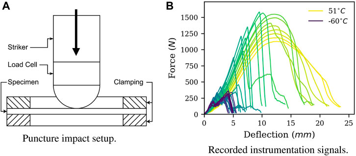
FIGURE 1. Puncture test setup (A) and recorded instrumentation signals (B) for an exemplary PE/PP compound. For polymers, a transition from ductile-to brittle fracture behavior can be observed at decreasing temperatures. Instrumentation signals are commonly referred to as ”force-deflection curves”.

Impact behavior of polyolefins has been extensively researched in literature. Noteworthy aspects influencing the DBTT include the microstructure morphology, specimen geometry and loading rate (Perkins, 1999). Additionally, the presence and shape of local defects has an influence on toughness (Huang et al., 2003). It has been shown by (Kunz-Douglass et al., 1980; Yee and Pearson, 1986) that plastic shear-yielding of the matrix is the main process of energy dissipation under impact loading. Furthermore, a dependence on the molecular weight (Van der Wal et al., 1998) and a related change in the DBTT caused by aging (Yang et al., 1996; Jose et al., 2014; Suarez and Mano, 2000) can be observed. The processing conditions of PE/PP blends was also found to affect the impact behavior (Strapasson et al., 2005). The toughness of polyolefins can be improved significantly by the addition of impact modifiers (Panda et al., 2015; Li et al., 1998; Tam et al., 1996). In (Tai et al., 2000), the impact behavior of PE/PP blends in various compositions is compared. The crystallinity influences the impact strength at low temperatures (Shao et al., 2015) and the strain-stress behavior under high loading rates up to 1,000 s⁻¹ (Zhu et al., 2022).

Data-based modelling approaches have emerged as effective alternative to analytical- or numerical investigations. Material science is challenged with many difficulties regarding the applicability of machine learning. In most scenarios, the availability of experimental data is a major problem due to expensive acquisition and a lack of public databases. Review papers summarizing the state of machine learning in various sectors of material science are available. For example, in continuum materials mechanics (Bock et al., 2019), solid state material science (Schmidt et al., 2019) or composite material design and discovery (Chen and Gu, 2019). Recent trends in polymer science are summarized in (Martin and Audus, 2023). To overcome the problem of insufficient experimental data, many studies generate artificial datasets by numeric or stochastic simulations (Reimann et al., 2019; Pitz et al., 2021; Paul et al., 2019; Wang et al., 2021). Exploration of real-world experimental datasets are uncommon in material science. In (Alidoust et al., 2021), machine learning models are established using a set of 153 cyclic triaxial tests to determine the shear modulus of municipal solid waste. Another example of machine learning on small experimental datasets is presented in (Altarazi et al., 2019), using cut samples from high density PE films produced at various process conditions to predict the Young’s modulus. In (Ho et al., 2021), the elastic modulus of carbon nanotube composites is predicted by neural networks trained on an experimental database of 282 materials. Likewise, a set of 82 dielectric materials has been utilized to build machine learning models able to predict the intrinsic dielectric breakdown field (Kim et al., 2016). Using a set of 40 notched uniaxial tensile tests at certain strain rates and temperatures, viscoelasticity of PE is described using an artificial neural network constitutive model (Jordan et al., 2020). In (Mallakpour et al., 2014), a set of 50 optically active polymers were investigated by thermogravimetric analysis to model quantitative structure-property relations with support vector machines. The application of regression trees was showcased in (Li, 2006), where 1,600 creep experiments were used to model the creep rupture life and rupture stress of austenitic stainless steels.

Polyolefin compound development still predominantly involves trial-and-error-based design of experiments, where large amounts of data are generated. IPTs are a common method to quantify the impact resistance, and ever-growing databases make it possible to utilize data-based modelling techniques. We expect that single IPTs can indirectly provide information about the time-temperature dependency of material behavior. For this reason, we apply machine learning algorithms to a database of 181 PE/PP compounds and 7,587 experiments. With a combination of Principal Component Analysis (PCA) and K-Means Clustering (KMC), we aim to demonstrate how unsupervised machine learning algorithms can identify meaningful structures or clusters within datasets. In a supervised regression setting, we utilize Random Forest Regressors (RFR) to predict DBTTs from single recorded instrumentation signals. This approach holds the potential to reduce costs and time for material characterization, enables fast screening of materials and offers the possibility to determine DBTTs without thermal specimen conditioning.

2 Materials and methods

As machine learning is data-driven, this section starts with an overview of the experimental database. This is followed by a description of the transition temperature determination. A general overview of applied machine learning methods and the validation process is presented in Section 2.3. Finally, we give detailled information about feature engineering, Principal Component Analysis, K-Means Clustering and Random Forest Regression.

2.1 Data acquisition

Our dataset is composed of 7,587 IPTs with consistent setup (International Organization for Standardization, 2020) and consistent specimen conditioning (International Organization for Standardization, 2016). Relevant parameters include a striker velocity of 4,400 mm s⁻¹, a specimen thickness of 2 mm, a striker diameter of 20 mm and a clamping ring diameter of 40 mm. Experiments are conducted with clamped specimens and with lubricated strikers. Data is structured in temperature sweeps, which refer to systematic variations of up to 56 experiments with test temperatures ranging from −60°C to 51 C for each material. In total, 181 recycled Polyethylene (PE) and Polypropylene (PP) compounds are examined. These base materials are combined with either impact modifiers, virgin homopolymers or Heterophasic-Copolymers (HECO) in weight fractions ranging from 5% to 40%. Materials are classified according to base materials into either PE, PP or PE/PP. In Table 1, the number of experiments for each material category is listed.

TABLE 1

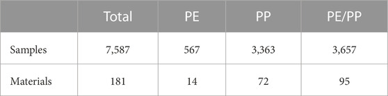
TABLE 1. Number of experiments and materials for respective categories.

2.2 Determination of transition temperatures

Although the transition from ductile-to brittle takes place over a temperature range, it is commonly characterized by a discrete Ductile-Brittle Transition Temperature (DBTT). To determine the DBTT, toughness related quantities are observed at multiple temperatures and a threshold is defined. In this study, we calculate the puncture energy E_p as area below the force-deflection curve. A characteristic progression of E_p over temperature T is shown in Figure 2. Energies are traditionally separated into Lower-Shelf (LS), Transition Region (TR) and Upper-Shelf (US) (Altstadt et al., 2016). We determine the DBTT by linear interpolation where puncture energy drops below 66% of the maximum upper shelf energy $E_p^{us}$. Since experimental results may scatter significantly, it is beneficial to utilize curve fitting- or filtering methods (Cao et al., 2012). We apply a gaussian filter with intensity σ = 2.0 to mitigate the effect of observed scatter on the resulting DBTTs.

FIGURE 2

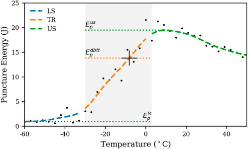
FIGURE 2. Determination of the Ductile-Brittle Transition Temperature (DBTT). Transitions are interpolated where puncture energy drops below 66% of the maximum upper shelf energy $E_p^{us}$. Energies are filtered to mitigate the influence of scatter on the resulting DBTTs.

2.3 Cross-validation

Machine learning models are trained (optimized), validated and tested on separate datasets. The splitting of data can lead to optimistic evaluations of the quality of predictions, which has to be considered when evaluating models. In this study, the base material categories from Table 1 are unevenly represented, which leads to high variance of observations. This increases the risk of overfitting models, meaning that models might fit perfectly to the training data but fail at generalization to unseen data (Cawley and Talbot, 2010). To address the issue of overfitting, we conduct cross-validation, where we divide the training data into five validation subsets called ”folds” (Krstajic et al., 2014). Each fold serves as validation set for a model that was trained on the other remaining folds. The performance of the resulting five models are quantified by scoring functions that compare the model outputs to desired target values. Average and standard deviation of validation scores correspond to model bias and variance. Low bias and variance is preferred. Data is randomly split by sweeps rather than single experiments to avoid information leakage as shown in Figure 3. We split subsets via stratification to ensure equal distributions of base materials across subsets. Cross-validation is conducted as follows, with more detailled descriptions in the upcoming sections.

• Separate a test set from the data (30%).

• Conduct cross-validation on remaining data (5-folds):

• Extract features from instrumentation signals. First, features of training data are standardized and then features of validation data are transformed to the same scale.

• Conduct Principal Component Analysis (PCA) on standardized features of training data and then transform the standardized features of validation data to the same coordinate system.

• Train a Random Forest Regressor (RFR), a Linear regression model (LIN) and a K-Means Cluster (KMC) model on principal components. RFR hyperparameters are optimized by nested cross-validation. LIN serves as baseline to assess the quality of RFR predictions.

• Evaluate predictions of LIN and RFR on the validation fold.

• Get the average validation performance of all models. Average and standard deviation reflects bias and variance. Low bias and variance are preferred.

• Combine the five cross-validated RFR-models in an ”ensemble” that outputs the median of submodel predictions. Evaluate the ensemble predictions on the test set. The KMC model is used to check for the applicability of predictions.

FIGURE 3

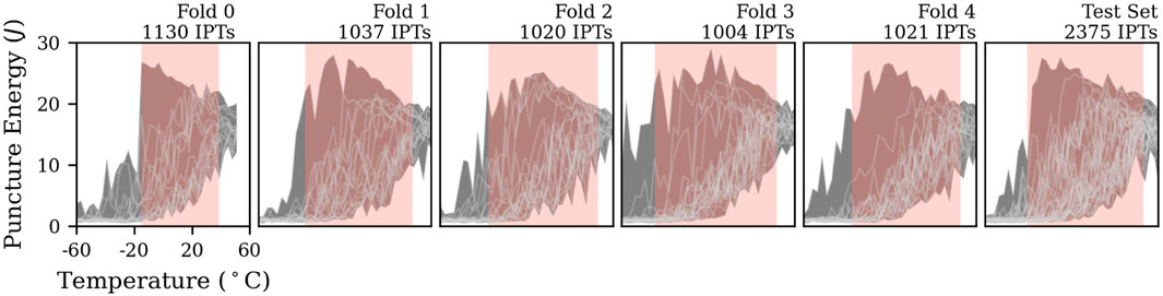
FIGURE 3. Machine learning requires the evaluation of trained models on separate sets of data. We randomly split the database by temperature sweeps into a test set and five cross-validation folds. Individual temperature sweeps and the bounding envelopes are displayed. Vertical boxes indicate the covered range of DBTTs in each set. Random forest regressors can hardly extrapolate outside of the data used for training. Stratification ensures equal distributions of base materials across subsets.

2.4 Feature engineering

In machine learning terminology, instrumentation signals are observations in the form of time-series. Any kind of information extracted from an observation is a feature as long as it helps a model to predict a specific target (Liu and Motoda, 1998). Feature engineering is a process of applied data-mining techniques and can be considered machine learning as well (Ng, 2018). Domain knowledge is essential in extracting features from time-series. It is favorable to generate a large and diverse set of features and then filter them according to their significance for the task at hand (Fulcher and Jones, 2014). A balance between meaningful and frail features (e.g., deflection at crack initiation) and robust but probably non-significant features (e.g., median of all force values) is preferable (Christ et al., 2016). Having too many features including irrelevant ones is better than missing out on important ones. However, models with unnecessary predictors are more prone to overfitting during training. In such scenarios, feature selection should be applied (Kuhn and Johnson, 2019). Our approach follows the same idea: we generate a set of features as diverse as possible and select a subset of features for training.

We split normalized force-deflection (F-s) curves into characteristic segments by determining points with the largest orthogonal distance to the direct connection lines between origin, peak load and breaking point as shown in Figure 4. This way, we define six distinct sections throughout puncture, which will be referenced by index i from 0 to 5. We extract statistical quantities within these partitions (Deng et al., 2013), for example, linear trends K_i determined by least squares regression. Also, the energy of individual sections E_i and their ratio to the total energy $R_i=\frac{E_i}{E}$ inspired by the ductility index (Yim et al., 2017) are considered. Other features derived from curve segments include mean ($F_i^{\mathit{avg}}$, $s_i^{\mathit{avg}}$), median ($F_i^{\mathit{med}}$, $s_i^{\mathit{med}}$), standard deviation $(F_i^{\mathit{std}})$, variance $(F_i^{\mathit{var}})$, skew and kurtosis (Wang et al., 2006) ($E_i^s$, $F_i^s$, $E_i^k$, $F_i^k$). Referenced without index, these features are also calculated for the whole time series. The peak load and the corresponding deflection (F^max, s^max) is determined as well. Finally, the number of local force maxima n_p is considered. This amounts to a total of 94 input variables. We considered extracting features from the frequency domain of the instrumentation signal (Mörchen, 2003), but disregard them in this study because the periodicity of the signals is limited. While normalization is conducted to divide force-deflection curves into subsections, features are calculated using the original non-normalized data. In the Supplementary Materials, we attach an exemplary. csv file of extracted features.

FIGURE 4

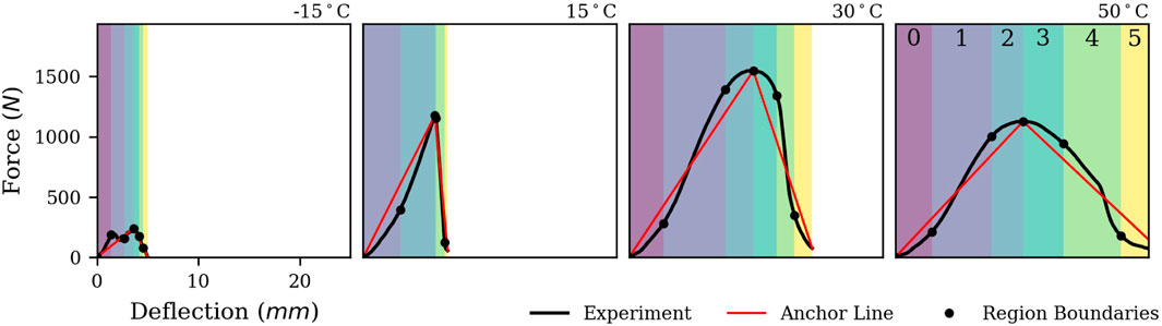
FIGURE 4. Feature engineering approach for an exemplary material at different temperatures. The force-deflection curves are segmented into characteristic regions. 94 statistical quantities are extracted from the force-, deflection- and energy distributions in the respective regions. These serve as inputs for machine learning models.

2.5 Target definition

Instead of using the DBTT directly, proposed models predict the temperature difference ΔT = T − DBTT between the test temperature T and the DBTT. This allows predictions to be a measure of the relative distance and direction rather than an absolute location on the temperature scale. The increased variability of the target can have a beneficial effect on training by amplifying prediction errors on outliers. Furthermore, it is not necessary to add temperature to the inputs of the model.

2.6 Principal Component Analysis

We expect high collinearity of features because deflection, force and energy are closely related. Real-world data shows a certain degree of collinearity and predictive capabilities of models are not necessarily affected by it (Shmueli, 2010). It is mainly a cause of concern regarding model explainability, because collinear variables share substantial amounts of information and small changes in features can strongly affect the outputs of the model (Dormann et al., 2013). There are different ways to check for collinearity. We calculate the determinant of the Pearson correlation matrix across all cross-validation folds. It is a symmetric matrix whose components are Pearson correlation coefficients that are a measure of linear correlation between two features (Freedman et al., 2007). In this case, a determinant below 1E-4 indicates strong multicollinearity. Contrary, a value of 1 would correspond to non-collinearity in the dataset (Field, 2013). Because of this excessive collinearity, tree-based or permutation feature importance metrics may give misleading results and will not be assessed in this study (Hooker and Mentch, 2019).

We apply Principal Component Analysis (PCA) with prior standardization of features to the training data in an effort to overcome multicollinearity (Upton and Cook, 2008). This is done by transforming features into a new coordinate system of linearly uncorrelated variables, called principal components (PC). These are ordered according to the amount of variance they explain in the original data, with the first component explaining the highest variance and the last principal component the lowest. The dimensionality of the dataset can then be reduced by dropping principal components with the lowest variance while retaining a certain amount of explained total variance. In this study, we keep a subset of principal components that hold 99.99% of variance in each training set in the cross-validation cycle. One downside of PCA is that information is lost upon transformation if not all components are considered. Furthermore, principle components are difficult to interpret.

PCs and their explained variance are represented by the eigenvectors and eigenvalues of the covariance matrix of original features in the training set. Observations in the validation- and test sets are then transformed to the same coordinate system. First, the same standardization of features as for the training data is conducted. Then, the PCs are calculated by multiplication with the matrix of eigenvectors of the training covariance matrix. We show an examplary PCA fitted on the training data of one cross-validation iteration in Figure 5. Here, the first three principal components shown in the diagrams explain 72% of variance in the training data.

FIGURE 5

FIGURE 5. Investigation of the dataset by Principal Component Analysis. In (A), temperature sweep regions LS (lower shelf, brittle), TL (transition region, below DBTT), TU (transition region, above DBTT) and US (upper shelf, ductile) can be related to material toughness. With (B) and (C), we show that experiments, base materials and DBTTs are balanced among dataset splits and that the test set is representative of the train data. In (D), numbers indicate cluster centroids from K-Means Clustering.

2.7 K-Means Clustering

K-Means Clustering (KMC) is an unsupervised machine learning algorithm used for separating data into k distinct clusters based on similarity or dissimilarity in the form distance metrics. The algorithm assigns each observation to the cluster C_i with the nearest center μ_i. Centers or ”centroids” are located at the mean of all cluster observations and are calculated as

${\mu }_i=\frac{1}{‖C_i‖}{\displaystyle \sum _{x_j\in C_i}}{x}_j,(1)$

with $‖C_i‖$ as number of observations, x_j as observations and C_i as the respective clusters. The dataset $D=\left\{x_i\right\}\subset X,i=1\dots N$ contains all observations. Initially, cluster centers are chosen randomly μ_i ∈ X. During training, they are iteratively optimized. KMC aims to minimize the within-cluster variances by minimization of the squared Euclidian distances. This process continues until convergence, when centroids stabilize and cluster assignments remain unchanged. This results in a partitioning of the data space into Voronoi cells. KMC is an efficient algorithm and due to its simplicity one of the most widely used clustering methods. It does not make assumptions about the distribution of features and works well on non-gaussian distributed data. However, KMC is not guaranteed to find optimal solutions and performance can be sensitive to the initial placement of centroids. There are various ways for the initialization of cluster centers (Hamerly and Elkan, 2002). We use the K-Means++ method, which improves the probability of obtaining optimal solutions in comparison to random initialization and shows faster convergence (Arthur and Vassilvitskii, 2007).

During cross-validation, we conduct KMC++ for the training data of each iteration with k = 5 clusters. We use the PCA transformed features as input. In Figure 5D, resulting cluster centers are visualized in the PCA coordinate system and indicated by enumeration. In the discussion section, we will examine the characteristics of these individual clusters. The displayed clusters are representative of all fitted KMC-models throughout cross-validation since they share substantial amounts of training data.

2.8 Random Forest Regression

A decision tree is a predictive model that connects input features to output targets by partitioning of the dataset. Random Forest Regressors (RFRs) are a combination of multiple decision trees and are based on the concepts of bootstrapping and bagging (Jacoby and Armstrong, 2014). Bootstrapping implies that each individual tree is fitted on random subsets of training data by sampling with replacement. Bagging transforms all trees into a meta-model ”forest” that outputs the average of submodel predictions. This is commonly referred to as bootstrap aggregation, which reduces training time and adds a regularization effect (Krogh and Vedelsby, 1994). The concept of bootstrap aggregation is depicted in Figure 6. We implement RFRs via the Scikit-Learn (Pedregosa et al., 2011) library in Python 3.8 (Van Rossum and Drake, 2009).

FIGURE 6

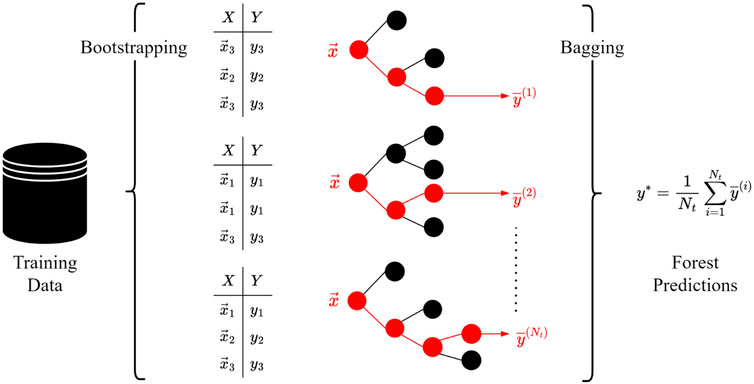
FIGURE 6. Bootstrap aggregation of Random Forest Regressor (RFR) as combination of decision trees. During bootstrapping, each tree is trained (optimized) on random subsets of training data by sampling with replacement. The predictions of all trained trees are averaged, which is referred to as bagging.

We paraphrase a brief explanation of classification- and regression trees from (Loh, 2011). Let $\overrightarrow{x_i}\in R^n$ and $\vec{y}\in R^l$ be the feature and target vector for observation i = 1, …l. The number of features is denoted with n. Decision trees recursively partition their training data in order to group observations with similar target values. These splits are conducted at nodes m that represent subsets of data Q_m with N_m observations. Possible candidates for splits θ = (j, t_m) with feature index j and threshold t_m are defined as

$Q_m^{\mathit{left}}\left(\theta \right)=\left\{\left(x,y\right)|x_j\le t_m\right\},(2)$

$Q_m^{\mathit{right}}\left(\theta \right)=Q_m\backslash Q_m^{\mathit{left}}\left(\theta \right),(3)$

with $Q_m^{\mathit{left}}$ and $Q_m^{\mathit{right}}$ as resulting subdivisions of the feature space. During model training, an error function H(Q_m) determines the quality of each split at node m. For regression tasks, the mean squared error (MSE) function is deployed as

$H\left(Q_m\right)=\frac{1}{N_m}{\displaystyle \sum _{y\in Q_m}}{\left(y-{\bar{y}}_m\right)}^2,(4)$

${\bar{y}}_m=\frac{1}{N_m}{\displaystyle \sum _{y\in Q_m}}y,(5)$

with the predicted value being the mean value of all datapoints in the node ${\bar{y}}_m$. The optimal split is determined by minimizing the combined error

$G\left(Q_m,\theta \right)=\frac{N_m^{\mathit{left}}}{N_m}H\left(Q_m^{\mathit{left}}\left(\theta \right)\right)+\frac{N_m^{\mathit{right}}}{N_m}H\left(Q_m^{\mathit{right}}\left(\theta \right)\right),(6)$

${\theta }^{*}=argmi{n}_{\theta }G\left(Q_m,\theta \right),(7)$

of the left and right split sides of the dataset. This procedure is recursively applied until either a stopping criteria is met or N_m = 1. The final node in each branch of the tree is referred to as leaf node. Decision tree regressors offer a variety of stopping criteria, for example, a maximum tree depth D^max or a minimum amount of observations for each split $N_s^{\mathit{min}}$. Alternatively, tree growth can be stopped by prescribing a minimum amount of leaf observations $N_l^{\mathit{min}}$. Candidate splits θ are usually restricted to a subset of $N_f^{\mathit{max}}$ features to further minimize the risk of overfitting models. A random forest encompasses a total number of N_t decision trees, each trained on a subset of $N_b^{\mathit{max}}$ observations (bootstrap size). Individual predictions of input $\vec{x}$ are averaged to a combined output y*.

Non-trainable parameters of machine learning models are referred to as hyperparameters. In this study, we optimize RFR hyperparameters via nested cross-validation (Hastie et al., 2009; Varma and Simon, 2006; Krstajic et al., 2014). Here, the training data of each ”outer” cross-validation iteration is further divided into three ”inner” subfolds where we apply a stepwise Bayesian optimization algorithm (Shahriari et al., 2015). In each of 100 steps, RFRs are trained with specific combinations of hyperparameters and validated via inner cross validation. The final optimized hyperparameters are selected according to the lowest average validation MSE. We compile all five cross-validation results in Table 2. Descriptions of hyperparameters are listed in Section 2.8 and can be looked up in the Scikit-Learn documentation (Pedregosa et al., 2011).

TABLE 2

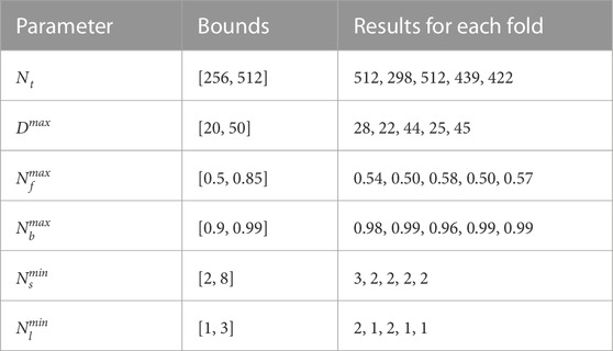
TABLE 2. Selected hyperparameters for the five RFRs trained troughout cross-validation.

3 Results

During cross-validation, five Random Forest Regressors (RFRs) with optimized hyperparameters are trained. Additionally, ordinary least-squares linear regression models (LIN) are fitted, which use the same input features and serve as baseline to assess the quality of predictions. In Table 3, we quantify the quality of predictions by the Root Mean Squared Error (RMSE). The average and standard deviation of RMSEs across validation- and test sets can be related to the bias and variance of RFR/LIN. Results on the test set are within the expected standard deviation range. High variance is caused by the unequal representation of the base material classes PE, PP and PE/PP across sets. Therefore, we combine all five RFR-models into one ”ensemble” that outputs the median of submodel predictions. In Table 4, we assess the quality of ensemble predictions on the test set by RMSE, Mean Absolute Error (MAE) and coefficient of determination (R2-score). For practical use cases, predictions of experiments conducted at Room Temperature (RT) are especially interesting because these do not require thermal specimen conditioning. Another subset that only considers observations in the Transition Region (TR) (Section 2.2) is selected.

TABLE 3

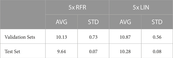
TABLE 3. Five Random Forest Regressors (RFR) and five Linear regressors (LIN) are trained throughout cross-validation and evaluated on the validation- and test sets. The resulting Root Mean Squared Error (RMSE) in °C of predictions compared to actual DBTTs are compiled.

TABLE 4

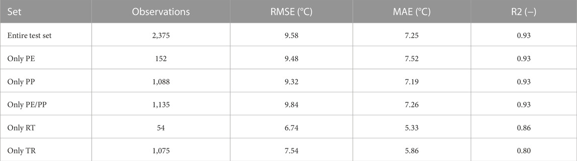
TABLE 4. Ensemble performance on test set. Separate evaluations for the base material categories PE, PP and PE/PP are conducted. Additionally, all Room Temperature (RT) and Transition Region (TR) observations of the test set are isolated.

4 Discussion

4.1 Clustering

To visualize the difference between clusters of Figure 5D, we display all corresponding force-deflection curves in Figure 7. We order cluster indices according to their average target values ΔT, starting with (i) brittle- and ending with (v) ductile experiments. These clusters are reminiscent of ISO 6603-2 (International Organization for Standardization, 2020) fracture categories. Representatives of cluster (ii) are predominantly PE-compounds as shown in Figure 5C, which emphasizes that their fracture behavior is distinct from compounds with PP contents. Both ISO categories and KMC clusters can be related to the characteristic temperature sweep regions in Figure 5A. This way, clustering affirms that ISO fracture types provide a meaningful and relevant framework for the impact behavior of polyolefins. It also shows that the applied feature engineering with PCA is effective in transforming the dataset of instrumentation signals to a coordinate system where fracture types are clearly separable. This linear separability of KMC clusters- (Figure 5A), ISO fracture types- and temperature sweep regions (Figure 5A) might explain why the performance of linear regressors compared to non-linear RFRs is only marginally reduced.

FIGURE 7

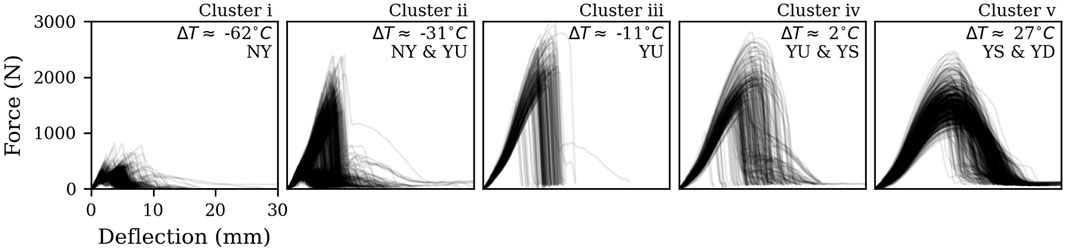
FIGURE 7. Force-deflection signals of all clusters obtained by KMC. Clusters are reminiscent of ISO 6603-2 fracture types Yielding with Deep drawing (YD), Yielding with Stable cracking (YS), Yielding with Unstable cracking (YU) and No Yielding (NY). The average ΔT of cluster representatives is displayed.

4.2 Predictions on the test set

The proposed models allow each individual force-deflection curve to make its own estimate of the transition temperature without further information of the underlying temperature sweep. In Figure 8, we compare the predictions of the ensemble to the actual DBTTs for all base material categories. Except for observations in direct proximity of the transition, models are able to consistently point into the direction of the DBTT. Predictions are systematically overestimating the DBTT in the lower shelf, where force-deflection curves are indistinguishable by humans. In general, predictions in the transition region are more accurate. We assume that observations hold more variance in this domain of the dataset, which facilitates increased capabilities to predict the variability of DBTTs. R2-scores of approximately 0.93 (Table 4) indicate that most of the variability of DBTTs is explained by the ensemble.

FIGURE 8

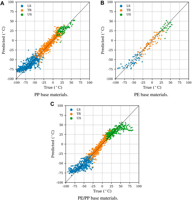
FIGURE 8. Ensemble predictions of ΔT = T-DBTT on the test set. For very brittle (Lower Shelf LS) and very ductile (Upper Shelf US) experiments, models are under- or overestimating DBTTs. In these domains, force-deflection curves become indistinguishable. Predictions in the Transition Region (TR) are more accurate. Selected results for PP- (A), PE- (B) and PE/PP (C) compounds are displayed.

4.3 Scaleability

In the introduction, we argue that proposed models could reduce time- and costs of material characterization by enabling predictions of DBTTs from single IPTs. We investigate this scenario by only considering experiments tested at Room Temperature (RT). In this case, the ensemble achieves a MAE of 5.3°C (Table 4) and predictions are consistently within 10°C of the actual DBTTs. We point out that 40 out of 54 IPTs are located in the Transition Region (TR) of their respective temperature sweeps. Here, predictions are generally more accurate because testing temperatures are closer to the actual DBTTs.

Despite the underrepresentation of PE in the training data, the ensemble’s quality of predictions is only marginally reduced for this subset of the database. This suggests that streamlined measurement studies of narrow material categories could allow for reasonable model performance while requiring only moderate amounts of training data. However, we emphasize that the examined polyolefin categories might share substantial amounts of information. Therefore, we cannot conclude a minimum number of experiments necessary for model training.

Presented models should only be applied to compounds with material constituents similar to those the model was trained on. Different base materials, ingredients or fillers may result in a decreased quality of predictions. We exemplify this in Figure 9, where we compare a PP basematerial from the test set to a 100% HECO and another HECO filled with 20% talcum. In the training data, filled compounds are not included and HECOs are only present in weight fractions up to 40%. Although the proposed model allows predictions for any IPT measurement, we do not recommend its application in cases like Figures 9B,C. We specifically advise against the usage in following cases: (i) If the puncture energy is smaller than 2.5 J (ii) If the puncture energy at the measurement temperature is outside the envelopes of train sets (Figure 3). (iii) If the squared Euclidian distance of examined observations in the PCA-coordinate system to their corresponding assigned KMC centroids is too large, which implies that force-deflection curves may be dissimilar to the train data. The threshold is set to the 90% quantile of cluster-center-distances in the train data. This check is conducted for each KMC fitted throughout cross-validation.

FIGURE 9

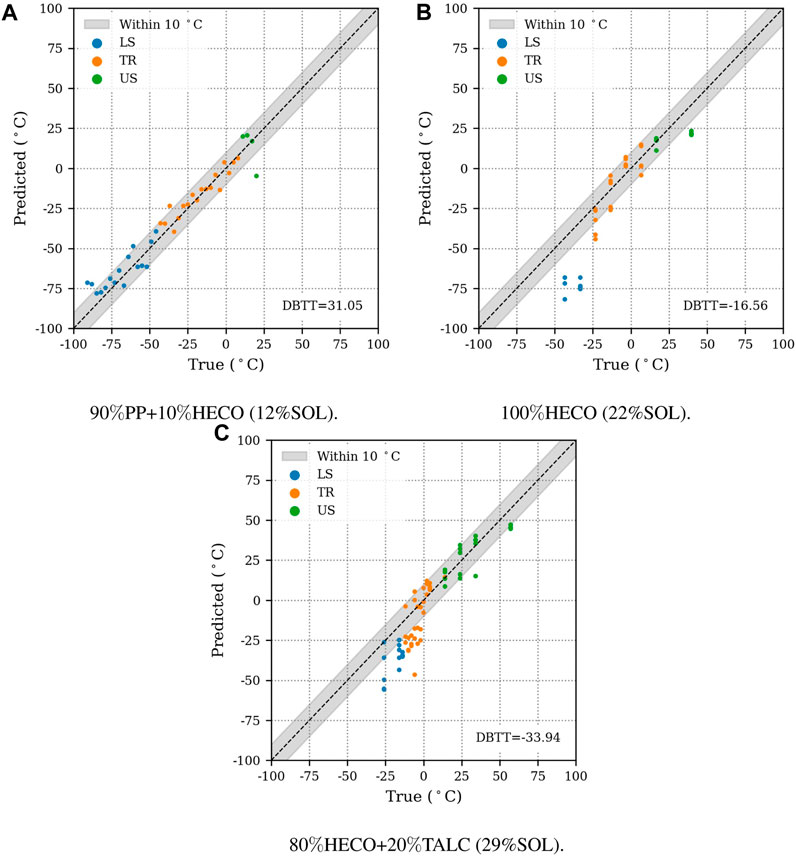
FIGURE 9. Ensemble predictions of ΔT = T-DBTT for selected materials. Bounding boxes indicate which predictions are within 10°C of the actual transition temperatures. (A) shows a temperature sweep from the test set. (B) and (C) show predictions for materials outside the scope of the training data. In such cases, the application of proposed models can yield decreased quality of results. The main difference between these materials is the soluble weight fraction (SOL), which is connected to amourphous rubber content.

4.4 Limitations

The proposed methodology is constrained by limitations of the IPT methodology: (i) According to the specimen conditioning norm, the actual specimen temperature may show variations of ±2°C in relation to the testing temperature (International Organization for Standardization, 2016). (ii) Injection molded specimens exhibit slight imperfections that influence the fracture process. Resulting scatter of puncture energy E_p can influence the determination of DBTTs. (iii) Deviations in the specimen thickness up to ±0.1 mm (International Organization for Standardization, 2020) should be expected. (iv) The instrumentation does not exclusively record the instrinsic material mechanical response but also includes inertia effects and high frequency noise of amplification systems (Menna, 2022).

While we apply RFRs in this study, other machine learning algorithms (Baştanlar and Özuysal, 2014) can also be successfully applied. Deep learning algorithms like convolutional-neural networks are just as capable of extracting relevant information from time-series, but pose many challenges when trained on small datasets. RFRs partition the training data space in a way that connects inputs-to the target output values. Decision-making purely depends on the similarity- or dissimilarity of force-deflection signals. Due to the regularization effect of bagging and bootstrapping, robust interpolation in regions with sufficient data in the feature space is possible. At the same time, extrapolation capabilities are very limited. We acknowledge that there is a need to understand and include underlying polymer physics. For example, information about molecular mass distributions or microstructure morphologies could be a suitable additional model input. Various other ways to incorporate domain knowledge into machine learning systems exist (Martin and Audus, 2023). To showcase the importance of microstructure information, we determine the soluble weight fraction (SOL) of the three materials displayed in Figure 9 by soluble fraction analysis (Monrabal and Ortín, 2013). For PE/PP compounds, the soluble- or amorphous fraction is usually related to elastomer content in the form of ethylene-propylene rubber (Wei et al., 2000). High SOL generally translates to tougher compounds. We find that the training database is missing observations in the domain of high SOL and low DBTTs respectively. While considerations of SOL and other morphology related quantities could significantly increase the extrapolation capabilities of models, soluble fraction analysis is not feasible for all 181 materials in the scope of this research due to sample availability. In future research, we aim to investigate fracture surface images of notched Charpy impact experiments in combination with instrumentation signals by machine learning algorithms. We suggest that plastic deformation mechanisms visible on the crack surface can be indirectly related to the morphology of materials.

4.5 Conclusions

We show that instrumented puncture impact tests can be related to the temperature dependency of polyolefin impact behavior. Utilization of supervised- and unsupervised machine learning algorithms on a database of 7,587 experiments proved valuable from a predictive and exploratory standpoint. We present a novel feature engineering method to extract 94 features from characteristic regions of recorded instrumentation signals. By applying Principal Component Analysis (PCA), this dataset was transformed to a new coordinate system where 72% of the variance is explained by the first three components. Application of K-Means Clustering (KMC) results in clusters that reflect ISO 6603-2 (International Organization for Standardization, 2020) fracture types, which validates the relevance of this categorization. Furthermore, the principal components proved suitable for reducing the dimensionality of the dataset while keeping relevant information for training machine learning models to predict the Ductile-Brittle Transition Temperature (DBTT). Based on this combination of feature engineering and PCA, the trained machine learning model achieves an R2-score of 0.93 on the test set. When considering only room temperature experiments in the test set, a mean absolute error of 5.3°C compared to the experimentally determined DBTTs is realized. These results suggest that predictions of DBTTs from single impact tests at room temperature allow for fast screening of materials and a drastic reduction of time and cost for compound development. Furthermore, estimations of the DBTT are possible without the need for thermal specimen conditioning.

This study exemplifies both the effectiveness and limitations of a purely data-driven approach and confirms that there is a need to understand the underlying structure-property relationship of polyolefin compounds. While we were able to show a strong correlation between the soluble weight fraction and the DBTT for selected materials, we could not measure this quantity for all materials due to sample availability. In future studies, we aim to investigate fracture surface images obtained from Charpy impact experiments by machine learning algorithms to incorporate information about plastic deformation- and fracture mechanisms during impact.

Data availability statement

The datasets presented in this article are not readily available because the data analyzed in this study was obtained from Boralis Polyolefine GmbH. Following licenses/restrictions apply: Intellectual Property Rights. Requests to access the datasets should be directed to JT, info@borealisgroup.com.

Author contributions

FK: Conceptualization, Methodology, Investigation, Visualization, Writing–original draft. MR: Conceptualization, Project administration, JT: Conceptualization, Validation, Resources, Writing–review and editing. MJ: Resources, Data curation, Project administration, Conceptualization. ZM: Supervision.

Funding

The author(s) declare financial support was received for the research, authorship, and/or publication of this article. Supported by Johannes Kepler Open Access Publishing Fund.

Conflict of interest

Authors JT and MJ were employed by Borealis Polyolefine GmbH.

The remaining authors declare that the research was conducted in the absence of any commercial or financial relationships that could be construed as a potential conflict of interest.

Publisher’s note

All claims expressed in this article are solely those of the authors and do not necessarily represent those of their affiliated organizations, or those of the publisher, the editors and the reviewers. Any product that may be evaluated in this article, or claim that may be made by its manufacturer, is not guaranteed or endorsed by the publisher.

Supplementary material

The Supplementary Material for this article can be found online at: https://www.frontiersin.org/articles/10.3389/fmats.2023.1275640/full#supplementary-material

References

Alidoust, P., Keramati, M., Hamidian, P., Amlashi, A. T., Gharehveran, M. M., and Behnood, A. (2021). Prediction of the shear modulus of municipal solid waste (MSW): an application of machine learning techniques. J. Clean. Prod. 303, 127053. doi:10.1016/j.jclepro.2021.127053

CrossRef Full Text | Google Scholar

Altarazi, S., Allaf, R., and Alhindawi, F. (2019). Machine learning models for predicting and classifying the tensile strength of polymeric films fabricated via different production processes. Materials 12, 1475. doi:10.3390/ma12091475

PubMed Abstract | CrossRef Full Text | Google Scholar

Altstadt, E., Ge, H., Kuksenko, V., Serrano, M., Houska, M., Lasan, M., et al. (2016). Critical evaluation of the small punch test as a screening procedure for mechanical properties. J. Nucl. Mater. 472, 186–195. doi:10.1016/j.jnucmat.2015.07.029

CrossRef Full Text | Google Scholar

Arthur, D., and Vassilvitskii, S. (2007). “K-means++ the advantages of careful seeding,” in Proceedings of the eighteenth annual ACM-SIAM symposium on discrete algorithms, 1027–1035.

Google Scholar

Baştanlar, Y., and Özuysal, M. (2014). Introduction to machine learning. miRNomics MicroRNA Biol. Comput. analysis 1107, 105–128. doi:10.1007/978-1-62703-748-8_7

CrossRef Full Text | Google Scholar

Bock, F. E., Aydin, R. C., Cyron, C. J., Huber, N., Kalidindi, S. R., and Klusemann, B. (2019). A review of the application of machine learning and data mining approaches in continuum materials mechanics. Front. Mater. 6, 110. doi:10.3389/fmats.2019.00110

CrossRef Full Text | Google Scholar

Cao, L., Wu, S., and Flewitt, P. (2012). Comparison of ductile-to-brittle transition curve fitting approaches. Int. J. Press. Vessels Pip. 93-94, 12–16. doi:10.1016/j.ijpvp.2012.02.001

CrossRef Full Text | Google Scholar

Cawley, G. C., and Talbot, N. L. (2010). On over-fitting in model selection and subsequent selection bias in performance evaluation. J. Mach. Learn. Res. 11, 2079–2107.

Google Scholar

Chen, C. T., and Gu, G. X. (2019). Machine learning for composite materials. MRS Commun. 9, 556–566. doi:10.1557/mrc.2019.32

CrossRef Full Text | Google Scholar

Christ, M., Kempa-Liehr, A. W., and Feindt, M. (2016). Distributed and parallel time series feature extraction for industrial big data applications. arXiv preprint arXiv:1610.07717.

Google Scholar

Deng, H., Runger, G., Tuv, E., and Vladimir, M. (2013). A time series forest for classification and feature extraction. Inf. Sci. 239, 142–153. doi:10.1016/j.ins.2013.02.030

CrossRef Full Text | Google Scholar

Dormann, C. F., Elith, J., Bacher, S., Buchmann, C., Carl, G., Carré, G., et al. (2013). Collinearity: a review of methods to deal with it and a simulation study evaluating their performance. Ecography 36, 27–46. doi:10.1111/j.1600-0587.2012.07348.x

CrossRef Full Text | Google Scholar

Field, A. (2013). Discovering statistics using IBM SPSS statistics. London, United Kingdom: sage, 444–445.

Google Scholar

Freedman, D., Pisani, R., and Purves, R. (2007). in Statistics (international student edition). Editor R. P. Pisani 4th edn. (New York: WW Norton and Company).

Google Scholar

Freudenthaler, P. J. (2022). Development of application-specific polyolefin recyclate compounds for packaging and pipe applications/author Paul j. freudenthaler.

Google Scholar

Fulcher, B. D., and Jones, N. S. (2014). Highly comparative feature-based time-series classification. IEEE Trans. Knowl. Data Eng. 26, 3026–3037. doi:10.1109/tkde.2014.2316504

CrossRef Full Text | Google Scholar

Grundstein, A., Meentemeyer, V., and Dowd, J. (2009). Maximum vehicle cabin temperatures under different meteorological conditions. Int. J. biometeorology 53, 255–261. doi:10.1007/s00484-009-0211-x

PubMed Abstract | CrossRef Full Text | Google Scholar

Hamerly, G., and Elkan, C. (2002). “Alternatives to the k-means algorithm that find better clusterings,” in Proceedings of the eleventh international conference on information and knowledge management, 600–607.

CrossRef Full Text | Google Scholar

Hastie, T., Tibshirani, R., and Friedman, J. (2009). The elements of statistical learning: data mining, inference, and prediction. Springer Science and Business Media.

Google Scholar

Ho, N. X., Le, T. T., and Le, M. V. (2021). Development of artificial intelligence based model for the prediction of young’s modulus of polymer/carbon-nanotubes composites. Mech. Adv. Mater. Struct. 29, 5965–5978. doi:10.1080/15376494.2021.1969709

CrossRef Full Text | Google Scholar

Hooker, G., and Mentch, L. (2019). Please stop permuting features: an explanation and alternatives. arXiv preprint arXiv:1905.03151.

Google Scholar

Huang, L., Pei, Q., Yuan, Q., Li, H., Cheng, F., Ma, J., et al. (2003). Brittle–ductile transition in PP/EPDM blends: effect of notch radius. Polymer 44, 3125–3131. doi:10.1016/s0032-3861(03)00205-2

CrossRef Full Text | Google Scholar

International Organization for Standardization (2016). Plastics - standard atmospheres for conditioning and testing. Geneva, Switzerland: Tech. Rep. ISO 291:2016.

Google Scholar

International Organization for Standardization (2020). Plastics - determination of puncture impact behaviour of rigid plastics - Part 2: instrumented impact testing. Geneva, Switzerland. Tech. Rep. ISO 6603-2:2000(en).

Google Scholar

Jacoby, W. G., and Armstrong, D. A. (2014). Bootstrap confidence regions for multidimensional scaling solutions. Am. J. Political Sci. 58, 264–278. doi:10.1111/ajps.12056

CrossRef Full Text | Google Scholar

Jordan, B., Gorji, M., and Mohr, D. (2020). Neural network model describing the temperature-and rate-dependent stress-strain response of polypropylene. Int. J. Plasticity 135, 102811. doi:10.1016/j.ijplas.2020.102811

CrossRef Full Text | Google Scholar

Jose, J., Nag, A., and Nando, G. (2014). Environmental ageing studies of impact modified waste polypropylene. Iran. Polym. J. 23, 619–636. doi:10.1007/s13726-014-0256-5

CrossRef Full Text | Google Scholar

Kim, C., Pilania, G., and Ramprasad, R. (2016). From organized high-throughput data to phenomenological theory using machine learning: the example of dielectric breakdown. Chem. Mater. 28, 1304–1311. doi:10.1021/acs.chemmater.5b04109

CrossRef Full Text | Google Scholar

Krogh, A., and Vedelsby, J. (1994). Neural network ensembles, cross validation, and active learning. Adv. neural Inf. Process. Syst. 7.

Google Scholar

Krstajic, D., Buturovic, L. J., Leahy, D. E., and Thomas, S. (2014). Cross-validation pitfalls when selecting and assessing regression and classification models. J. Cheminformatics 6, 10–15. doi:10.1186/1758-2946-6-10

PubMed Abstract | CrossRef Full Text | Google Scholar

Kuhn, M., and Johnson, K. (2019). Feature engineering and selection: a practical approach for predictive models. Boca Raton: CRC Press.

Google Scholar

Kunz-Douglass, S., Beaumont, P., and Ashby, M. (1980). A model for the toughness of epoxy-rubber particulate composites. J. Mater. Sci. 15, 1109–1123. doi:10.1007/bf00551799

CrossRef Full Text | Google Scholar

Li, W., Li, R., and Tjong, S. (1998). Fracture toughness of elastomer-modified polypropylene: material characterisation. Polym. Test. 16, 563–574. doi:10.1016/s0142-9418(97)00027-5

CrossRef Full Text | Google Scholar

Li, Y. (2006). Predicting materials properties and behavior using classification and regression trees. Mater. Sci. Eng. A 433, 261–268. doi:10.1016/j.msea.2006.06.100

CrossRef Full Text | Google Scholar

Liu, H., and Motoda, H. (1998). Feature Extraction, Construction and Selection: A Data Mining Perspective. Berlin Heidelberg, Germany: Springer.

Google Scholar

Loh, W. Y. (2011). Classification and regression trees. Wiley Interdiscip. Rev. Data Min. Knowl. Discov. 1, 14–23. doi:10.1002/widm.8

CrossRef Full Text | Google Scholar

Mallakpour, S., Hatami, M., Khooshechin, S., and Golmohammadi, H. (2014). Evaluations of thermal decomposition properties for optically active polymers based on support vector machine. J. Therm. Analysis Calorim. 116, 989–1000. doi:10.1007/s10973-013-3587-0

CrossRef Full Text | Google Scholar

Major, Z., Stelzer, P. N., and Kiehas, F. (2022). Impact loading and testing. Characterization and Failure Analysis of Plastics. Editor T. J. Menna (Almere, Netherlands: ASM International), 306–327. doi:10.31399/asm.hb.v11b.a0006919

CrossRef Full Text | Google Scholar

Martin, T., and Audus, D. (2023). Emerging trends in machine learning: a polymer perspective. Washington, DC: ACS Polymers Au.

Google Scholar

T. J. Menna (Editor) (2022). Characterization and failure analysis of plastics (ASM International). doi:10.31399/asm.hb.v11b.9781627083959

CrossRef Full Text | Google Scholar

Monrabal, B., and Ortín, A. (2013). Soluble fraction analysis characterization of the whole polymer, amorphous and a Quality Control Laboratory. Valencia, Spain: Polymer Char. Available at: https://api.semanticscholar.org/CorpusID:160003756.

Google Scholar

Mörchen, F. (2003). Time series feature extraction for data mining using DWT and DFT.

Google Scholar

Ng, A. (2018). Machine learning and AI via brain simulations. Available at: https:// datascienceassn.org/sites/default/files/Machine%20Learning%20and%20AI%20via%20Brain%20Simulations.pdf.

Google Scholar

Panda, B. P., Mohanty, S., and Nayak, S. K. (2015). Mechanism of toughening in rubber toughened polyolefin—a review. Polymer-Plastics Technol. Eng. 54, 462–473. doi:10.1080/03602559.2014.958777

CrossRef Full Text | Google Scholar

Paul, A., Mozaffar, M., Yang, Z., Liao, Wk, Choudhary, A., Cao, J., et al. (2019). A real-time iterative machine learning approach for temperature profile prediction in additive manufacturing processes. 2019 IEEE Int. Conf. Data Sci. Adv. Anal. (DSAA) (IEEE), 541–550. doi:10.1109/DSAA.2019.00069

CrossRef Full Text | Google Scholar

Pedregosa, F., Varoquaux, G., Gramfort, A., Michel, V., Thirion, B., Grisel, O., et al. (2011). Scikit-learn: machine learning in Python. J. Mach. Learn. Res. 12, 2825–2830.

Google Scholar

Perkins, W. G. (1999). Polymer toughness and impact resistance. Polym. Eng. Sci. 39, 2445–2460. doi:10.1002/pen.11632

CrossRef Full Text | Google Scholar

Pitz, E., Rooney, S., and Pochiraju, K. (2021). Modeling and calibration of uncertainty in material properties of additively manufactured composites. doi:10.12783/asc36/35758

CrossRef Full Text | Google Scholar

Reimann, D., Nidadavolu, K., Vajragupta, N., Glasmachers, T., Junker, P., Hartmaier, A., et al. (2019). Modeling macroscopic material behavior with machine learning algorithms trained by micromechanical simulations. Front. Mater. 6, 181. doi:10.3389/fmats.2019.00181

CrossRef Full Text | Google Scholar

Schmidt, J., Marques, M. R. G., Botti, S., and Marques, M. A. L. (2019). Recent advances and applications of machine learning in solid-state materials science. npj Comput. Mater. 5, 83. doi:10.1038/s41524-019-0221-0

CrossRef Full Text | Google Scholar

Shahriari, B., Swersky, K., Wang, Z., Adams, R. P., and De Freitas, N. (2015). Taking the human out of the loop: a review of bayesian optimization. Proc. IEEE 104, 148–175. doi:10.1109/jproc.2015.2494218

CrossRef Full Text | Google Scholar

Shao, Y., Wu, C., Cheng, S., Zhou, F., and Yan, H. (2015). Effects of toughening propylene/ethylene graft copolymer on the crystallization behavior and mechanical properties of polypropylene random-copolymerized with a small amount of ethylene. Polym. Test. 41, 252–263. doi:10.1016/j.polymertesting.2014.12.008

CrossRef Full Text | Google Scholar

Shmueli, G. (2010). To explain or to predict? Stat. Sci. 25 (3), 289–310. doi:10.1214/10-sts330

CrossRef Full Text | Google Scholar

Strapasson, R., Amico, S., Pereira, M., and Sydenstricker, T. (2005). Tensile and impact behavior of polypropylene/low density polyethylene blends. Polym. Test. 24, 468–473. doi:10.1016/j.polymertesting.2005.01.001

CrossRef Full Text | Google Scholar

Suarez, J. C. M., and Mano, E. B. (2000). Brittle–ductile transition of gamma-irradiated recycled polyethylenes blend. Polym. Test. 19, 607–616. doi:10.1016/s0142-9418(99)00031-8

CrossRef Full Text | Google Scholar

Tai, C., Li, R. K., and Ng, C. (2000). Impact behaviour of polypropylene/polyethylene blends. Polym. Test. 19, 143–154. doi:10.1016/s0142-9418(98)00080-4

CrossRef Full Text | Google Scholar

Tam, W., Cheung, T., and Li, R. (1996). An investigation on the impact fracture characteristics of EPR toughened polypropylene. Polym. Test. 15, 363–380. doi:10.1016/0142-9418(95)00041-0

CrossRef Full Text | Google Scholar

Upton, G. J. G., and Cook, I. (2008). A dictionary of statistics. Oxford University Press.

Google Scholar

Van der Wal, A., Mulder, J., Thijs, H., and Gaymans, R. (1998). Fracture of polypropylene: 1. The effect of molecular weight and temperature at low and high test speed. Polymer 39, 5467–5475. doi:10.1016/s0032-3861(97)10278-6

CrossRef Full Text | Google Scholar

Van Rossum, G., and Drake, F. L. (2009). Python 3 reference manual. Scotts Valley, CA: CreateSpace.

Google Scholar

Varma, S., and Simon, R. (2006). Bias in error estimation when using cross-validation for model selection. BMC Bioinforma. 7, 91. doi:10.1186/1471-2105-7-91

PubMed Abstract | CrossRef Full Text | Google Scholar

Wang, X., Smith, K., and Hyndman, R. (2006). Characteristic-based clustering for time series data. Data Min. Knowl. Discov. 13, 335–364. doi:10.1007/s10618-005-0039-x

CrossRef Full Text | Google Scholar

Wang, Y., Oyen, D., Guo, W. G., Mehta, A., Scott, C. B., Panda, N., et al. (2021). StressNet-Deep learning to predict stress with fracture propagation in brittle materials. npj Mater. Degrad. 5, 6–10. doi:10.1038/s41529-021-00151-y

CrossRef Full Text | Google Scholar

Wei, G. X., Sue, H. J., Chu, J., Huang, C., and Gong, K. (2000). Toughening and strengthening of polypropylene using the rigid-rigid polymer toughening concept part ii toughening mechanisms investigation. J. Mater. Sci. 35, 555–566. doi:10.1023/a:1004759923659

CrossRef Full Text | Google Scholar

G. Wolfgang, and S. Sabine (Editors) (2001). Deformation and fracture behaviour of polymers (Springer Berlin Heidelberg). doi:10.1007/978-3-662-04556-5

CrossRef Full Text | Google Scholar

Yang, A. M., Wang, R., and Lin, J. (1996). Ductile-brittle transition induced by aging in poly(phenylene oxide) thin films. Polymer 37, 5751–5754. doi:10.1016/S0032-3861(96)00395-3

CrossRef Full Text | Google Scholar

Yee, A., and Pearson, R. (1986). Toughening mechanisms in elastomer-modified epoxies. J. Mater. Sci. 21, 2462–2474. doi:10.1007/bf01114293

CrossRef Full Text | Google Scholar

Yim, Y. J., Rhee, K. Y., and Park, S. J. (2017). Fracture toughness and ductile characteristics of diglycidyl ether of bisphenol-a resins modified with biodegradable epoxidized linseed oil. Compos. Part B Eng. 131, 144–152. doi:10.1016/j.compositesb.2017.07.047

CrossRef Full Text | Google Scholar

Zhu, T., Li, X., Zhao, X., Zhang, X., Lu, Y., and Zhang, L. (2022). Stress-strain behavior and corresponding crystalline structures of four types of polyethylene under a wide range of strain rates. Polym. Test. 106, 107460. doi:10.1016/j.polymertesting.2021.107460

CrossRef Full Text | Google Scholar