Creep subsidence prediction algorithm considering the effect of stress history for subgrades

1 Introduction

The filler of subgrade is generally earth-rock mixtures, which are composed of fine-grain soil such as clay and coarse-grain soil such as gravel. Thus, the creep properties of coarse grain and fine grain soils decide jointly the subsidence of subgrade. The consolidation lines of fine-grain soil are often drawn on the semi-logarithmic coordinate in soil mechanics because the creep part of the curves is almost straight (Bai et al., 2019; Bai et al., 2021; Wang et al., 2022). A large number of experimental results have shown that the consolidation lines of coarse grain soil are perhaps not suitable for drawing on the semi-logarithmic coordinate, but it can be well described by the power function model (Kuwano and Jardine, 2002; Cheng and Ding, 2007; Sun et al., 2016; Huang et al., 2023). However, when the power function model is used to explain the consolidation lines of fine-grain soil, the long-term trend of creep deformation is not satisfactory (Briaud and Garland, 1985; Briaud and Gibbens, 1999; Bi et al., 2019). Therefore, if the power function model is used to explain the creep strain of fine-grain and coarse-grain soils in a uniform manner, it needs to be modified.

It has been debated for decades whether creep is generated in the process of primary consolidation. There are two opposing views. According to Hypothesis A, creep is generated only in the process of secondary consolidation, while creep is generated both in the process of primary consolidation and secondary consolidation according to Hypothesis B. Proponents of both views have proposed theoretical explanations. For example, scholars holding the view of Hypothesis A believe that creep is a consecutive process of decreasing volume with time under constant effective stress (Mesri and Choi, 1985; Mesri, 2009; Feng, 2010), whereas scholars supporting Hypothesis B argue that creep is an intrinsic property of granular materials, including soils, and occurs at any stage of consolidation (Bjerrum, 1967; Stolle et al., 1999; Yin, 1999; Karim et al., 2010; Yao et al., 2013). However, Degago et al. (2011) demonstrate that Hypothesis B is more consistent with the experimental law after analyzing data from numerous sets of consolidation tests and field experiments.

In this paper, the power function model is modified and the reasonableness of the modified power function model (called MPF model below) is verified by indoor experiment data of silty clay and earth-rock mixtures. Based on the MPF model and Bjerrum’s reclassification of consolidation, two one-dimensional creep deformation formulas were proposed. Two simplified algorithms to predict creep subsidence were developed on the basis of these two formulas, which are the prediction algorithm considering the stress history and the prediction algorithm without considering the stress history. Finally, the feasibility of the two prediction algorithms was confirmed by using the field monitoring data of creep subsidence from three sections of the subgrade of the Haolebaoji-Ji’an Railway. Meanwhile, the reliability and accuracy of the two prediction algorithms were verified by comparing the prediction results with two widely used subsidence prediction algorithms in practical engineering.

2 Theoretical basis

2.1 The MPF model

Numerous consolidation tests have shown that the compression curves are not unique but are essentially parallel to each other in a cluster of curves (Crawford, 1964; Yao et al., 2013). Bjerrum (1967) confirmed this law and referred to these parallel lines as ‘time lines’. Assuming there exists an instant normal compression line (INCL) with a creep time of zero, Yao et al. (2013) established the UH model considering the time effect. INCL is used as a reference line to reflect the stress history, which is plotted as a solid blue line in Figure 1. The points on INCL indicate that the soil element is normally consolidated soil without any creep. Since there is a limit to creep, there is also a limit to the creep deformation in Figure 1 (Yao and Fang, 2019). The limit of creep deformation under different loads is named Stable Normal Compression Line (SNCL), which is plotted as a blue dotted line in Figure 1.

FIGURE 1

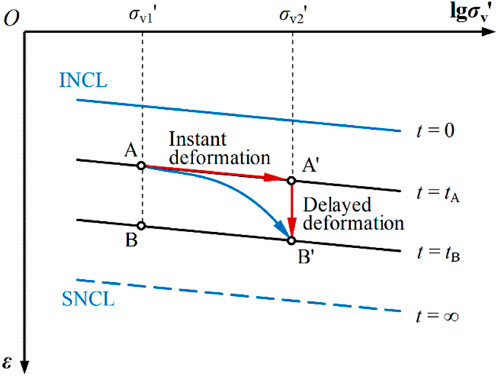
FIGURE 1. Schematic diagram of timelines and deformation.

From Hypothesis B of creep, it is clear that the consolidation deformation of soil elements is practically caused by the mixture of an increase in effective stress and an increase in time. A new definition of instant compression and delayed compression was established by Bjerrum to clarify the deformation due to multiple factors. Point A to point A′ in Figure 1 is represented as instant compression. In this compression process, we assume that the pore water pressure dissipates instantaneously and the skeleton composed of soil particles bears all loads instantaneously. Point A′ to point B′ in Figure 1 is represented as delayed compression, in which the soil skeleton is assumed to creep only with time. The deformation in these two compression processes is referred to as instant deformation and delayed deformation, respectively.

The power function model is often used to calculate the creep strain of fine-grain soils such as clay and silty fine sand (Briaud and Garland, 1985; Briaud and Gibbens, 1999; Bi et al., 2019). The commonly used formula of the power function model is (1)

$\frac{{\epsilon }_t}{{\epsilon }_1}={\left(\frac{t}{t_1}\right)}^n(1)$

where t is the time that creep lasts; t₁ is the unit reference time, generally expressed as 1s, 1min, or 1d; ε_t and ε₁ are creep strain at time t and t₁, respectively; n is the creep index.

According to Bjerrum’s division of the consolidation process, the delayed deformation includes the creep deformation in the primary consolidation process. As the focus is on creep, Eq. 1 is used to describe the delayed deformation without considering consolidation. Equation 1 indicates that in the bi-logarithmic coordinate, the deformation versus time is linear with a slope of n. However, as time t grows, creep deformation will keep growing until infinity. The true creep deformation law is that the creep rate decreases to zero as time t increases. The mathematical description is that the deformation-time curve will eventually be parallel to the time axis. Therefore, the MPF model can be expressed as:

$\frac{{\epsilon }_{t\infty }-{\epsilon }_t}{{\epsilon }_{t\infty }}={\left(\frac{t}{t_0}+1\right)}^{-n}(2)$

where ε_t is creep strain; ε_t∞ is creep strain when creep time is infinite; t₀ is the unit time used to unify the dimension of Eq. 1 and its value is one for the same dimension as creep time t; n is creep index dependent on the physical properties of soil.

By transforming Eq. 2, the expression of creep deformation ε_t can be obtained as:

${\epsilon }_t={\epsilon }_{t\infty }\left[1-{\left(\frac{t}{t_0}+1\right)}^{-n}\right](3)$

According to Eq. 3, ε_t is zero when t is zero and ε_t increases to ε_t∞ when t is infinite. That is, the creep strain increases non-linearly with creep time t to the limit ε_t∞. When ε_t∞ is constant, creep index n controls the rate of creep deformation. Figure 2. Shows a diagram of the creep curves based on Eqs 1, 3. As can be seen from Figure 2, the MPF model is more consistent with the creep law of soil.

FIGURE 2

FIGURE 2. Schematic diagram for power function model and MPF model.

The value of strain measured by the dial indicator in the consolidation test is total strain. The creep deformation ε_t in Eq. 3 is only the delayed deformation. So, the formula of total strain ε is

$\epsilon ={\epsilon }_t+{\epsilon }_{\text{ep}}(4)$

where ε_ep is the strain without creep, which is equivalent to instant deformation.

Similarly, the difference between the limit of total deformation ε_∞ and the limit of creep deformation ε_t∞ is ε_ep. Thus, the expression of ε_∞ is given as

${\epsilon }_{\infty }={\epsilon }_{t\infty }+{\epsilon }_{\text{ep}}(5)$

where ε_∞ is the limit of total strain when t is infinite.

Combining Eqs 3–5 yields:

$\epsilon ={\epsilon }_{\infty }-\left({\epsilon }_{\infty }-{\epsilon }_{\text{ep}}\right){\left(\frac{t}{t_0}+1\right)}^{-n}(6)$

According to Eq. 6, ε is ε_ep when t = 0, i.e., total strain is instant deformation at the beginning. When t is infinite, ε increases to ε_∞, i.e., the total strain increases non-linearly with time to a stable value ε_∞.

2.2 The verification of the MPF model

Equation 6 yields

${\epsilon }_{\infty }-\epsilon =\left({\epsilon }_{\infty }-{\epsilon }_{\text{ep}}\right){\left(\frac{t}{t_0}+1\right)}^{-n}(7)$

Equation 7 yields

$\mathit{lg}\left(\frac{{\epsilon }_{\infty }-\epsilon }{{\epsilon }_{\infty }}\right)=\mathit{lg}\left(\frac{{\epsilon }_{\infty }-{\epsilon }_{\text{ep}}}{{\epsilon }_{\infty }}\right)-n\mathit{lg}\left(\frac{t}{t_0}+1\right)(8)$

Equation 8 indicates that in bi-logarithmic coordinates, deformation versus time is also linear with a slope of -n. For clays, ε_ep is the strain corresponding to the point where the primary and secondary consolidation divides. The strain ε_ep can be determined by the ε-lgt curve obtained through consolidation tests. For earth-rock mixtures, there is no generally accepted standard for dividing instant deformation and delayed deformation. At present, the deformation value of 1 h under the last load is often used as the demarcation between instant and creep deformation of earth-rock mixtures (Cheng and Ding, 2007; Sun et al., 2016; Huang et al., 2023). If test data at 1 h is not available, the first measured deformation value after 1 h is used as an approximation of ε_ep. Currently, there are two methods for identifying the value of ε_∞: (i) The same soil is prepared into soil elements with different over-consolidated ratios and subjected to one-dimensional compression creep tests and one-dimensional expansion creep tests, respectively. The location of SNCL is then determined according to the relationship between the creep deformation and the over-consolidated ratio. In turn, the ε_∞ under the corresponding load can be determined (Yao et al., 2013; Yao and Fang, 2019). (ii) The ε_∞ is one of the parameters to be solved, which will be determined by optimization calculation. The first method to determine ε_∞ is more complicated because it requires multiple creep tests. Therefore, the second one is selected.

Huang et al. (2023) used silty clay and Zhang et al. (2021) used three kinds of earth-rock mixtures to carry out consolidation tests. These experimental data were re-plotted under semi-logarithmic coordinates, as detailed in Figure 3.

FIGURE 3

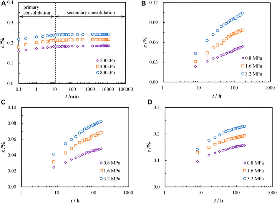
FIGURE 3. The experimental data of different soils replotted in the ε-lgt coordinate: (A) clay; (B) earth-rock mixture of sample 1; (C) earth-rock mixture of sample 2; (D) earth-rock mixture of sample 3.

According to Figure 3A, the secondary consolidation part of clay’s experimental data under different stress levels is linear and with essentially the same slope. According to Figures 3B–D, the creep part of the experimental data of three kinds of earth-rock mixtures is essentially nonlinear, but the trends of deformation are broadly similar. Due to the lack of deformation data between 0 and 8 h in Zhang et al. (2021), the deformation corresponding to the 8th hour, which is also the first deformation data in Fig. 10, is used as the demarcation between instant and creep deformation. Through these test data, the parameters ε_ep, ε_∞, and n in Eq. 8 are determined, as shown in Table 1 and Table 2. Combined with the parameters in the two tables, these experimental data were sorted based on Eq. 8 and then replotted in bi-logarithmic coordinates, as shown in Figure 4.

TABLE 1

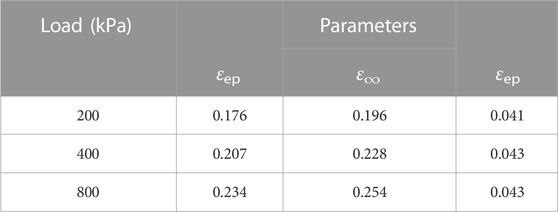
TABLE 1. Creep formula parameters of different soil elements.

TABLE 2

TABLE 2. Creep formula parameters of different soil elements.

FIGURE 4

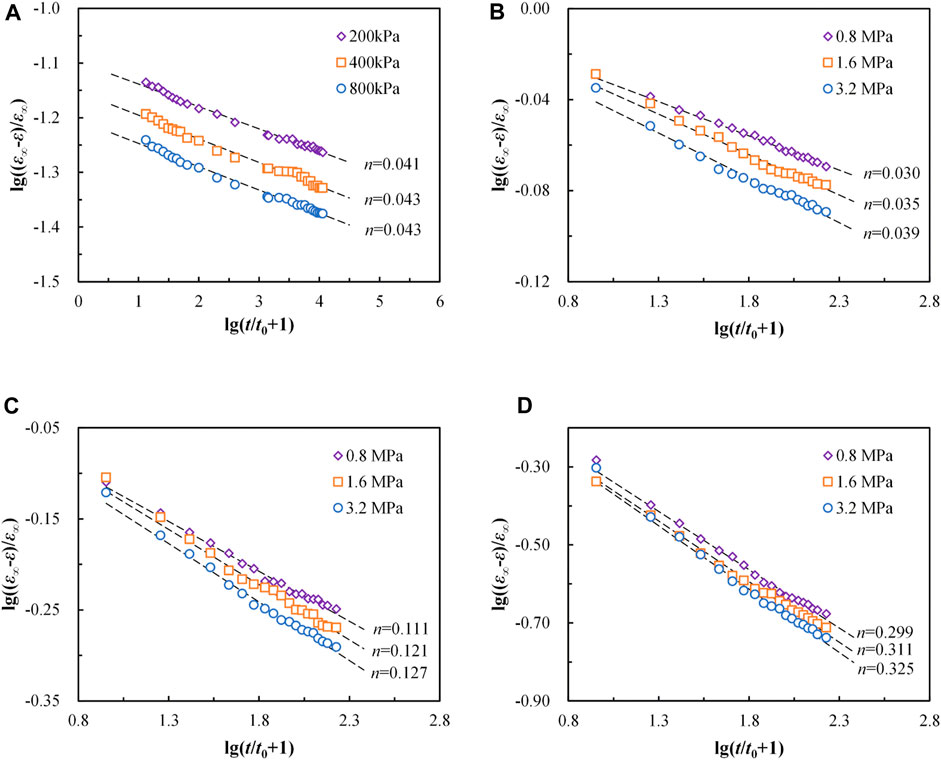
FIGURE 4. The experimental data of different soils replotted in the lg ((ε_∞-ε)/ε_∞)-lg (t/t₀+1) coordinate: (A) clay; (B) earth-rock mixture of sample 1; (C) earth-rock mixture of sample 2; (D) earth-rock mixture of sample 3.

According to Figure 4, these rearranged experimental data for different soil samples at various stress levels are almost straight with essentially the same slope. This shows that Eq. 8 derived on the basis of the MPF model is consistent with the creep characteristics of granular materials. Therefore, the MPF model is suitable for creep calculations of subgrade soils.

2.3 Creep deformation formulas

2.3.1 Creep deformation formula without considering stress history

When the state point lies on the reference line INCL, as in point A in Figure 5, the soil element is in a normal consolidated state. There has been no creep of any time in history. ε_λ and ε denote the instant and total strain of normal consolidated soil elements under an effective stress σ_v1', respectively. At this point, the instant deformation ε_ep of the normal consolidated soil element is ε_λ. Based on the MPF model and Bjerrum’s reclassification, the creep strain ε_t of a normal consolidated soil element from point A after time t is obtained from Eq. 6 as:

${\epsilon }_t=\epsilon -{\epsilon }_{\lambda }=\left({\epsilon }_{\infty }-{\epsilon }_{\lambda }\right)-\left({\epsilon }_{\infty }-{\epsilon }_{\lambda }\right){\left(\frac{t}{t_0}+1\right)}^{-n}(9)$

FIGURE 5

FIGURE 5. Schematic diagram for the creep of normally consolidated soil.

According to Eq. 9, ε_t is zero when t is zero, and ε_t is (ε_∞-ε_λ) when t is infinite. That is, creep strain ε_t increases non-linearly with time to the maximum deformation (ε_∞-ε_λ).

2.3.2 Creep deformation formula considering stress history

When the state point B lies below the INCL, as shown in Figure 6, the soil element is in an over-consolidated state. The load is unloaded from σ_v2' to σ_v1' and then held constant; C_c and C_s are the slopes of INCL and reload lines, respectively. ε_ep is the instant strain corresponding to point B. t_a is the equivalent creep time of the current state point with respect to the INCL. For state point B, t_a is the equivalent creep time between point A and point B.

FIGURE 6

FIGURE 6. Schematic diagram for the creep of over-consolidated soil.

From the analysis of Figure 6, it can be seen that starting creep from the current state point B after time t, the corresponding creep strain ε_t is:

${\epsilon }_t=\epsilon -{\epsilon }_{\text{ep}}=\left({\epsilon }_{\infty }-{\epsilon }_{\text{ep}}\right)-\left({\epsilon }_{\infty }-{\epsilon }_{\lambda }\right){\left(\frac{t+t_a}{t_0}+1\right)}^{-n}(10)$

where t_a is the equivalent creep time of the current state point relative to the reference line INCL.

When the normal consolidated soil element experiences the creep of time t_a from point A to point B, the strain of point B can be obtained from Eq. 6:

${\epsilon }_{\text{ep}}={\epsilon }_{\infty }-\left({\epsilon }_{\infty }-{\epsilon }_{\lambda }\right){\left(\frac{t+t_a}{t_0}+1\right)}^{-n}(11)$

From Eq. 11, the expression of t_a can be obtained as:

$t_a=t_0{\left(\frac{{\epsilon }_{\infty }-{\epsilon }_{\text{ep}}}{{\epsilon }_{\infty }-{\epsilon }_{\lambda }}\right)}^{-\frac{1}{n}}-t_0(12)$

Substituting Eq. 12 into Eq. 10 yields:

${\epsilon }_t=\left({\epsilon }_{\infty }-{\epsilon }_{\text{ep}}\right)-\left({\epsilon }_{\infty }-{\epsilon }_{\lambda }\right){\left[\frac{t}{t_0}+{\left(\frac{{\epsilon }_{\infty }-{\epsilon }_{\text{ep}}}{{\epsilon }_{\infty }-{\epsilon }_{\lambda }}\right)}^{-\frac{1}{n}}\right]}^{-n}(13)$

From Eq. 13, ε_t is zero when t is zero, and ε_t is (ε_∞-ε_ep) when t is infinite. That is, creep deformation ε_t increases non-linearly with time to the maximum deformation (ε_∞-ε_ep) in an over-consolidated state. It should be noted that after the same creep time t, the creep deformation ε_t between Figure 5 and Figure 6 are different. For the same soil, the void ratio in the over-consolidated state is smaller than that in the normal consolidated state. The creep rate of over-consolidated soil is smaller than that of normal consolidated soil under the same load σ_v1'. Therefore, the ε_t of the over-consolidated soil element in Figure 6 is smaller than that of the normal consolidated soil element in Figure 5, after experiencing the same creep time t.

The parameters ε_λ, ε_ep, ε_∞, n in Eq. 9 and Eq. (13) can be ascertained by one-dimensional creep tests (Bi et al., 2019; Huang et al., 2023). The creep strain ε_t of normal consolidated soil element and over-consolidated soil element is therefore only time-dependent. Let α = ε_∞-ε_ep, β = ε_∞-ε_λ, then Eq. 9 and Eq. (13) are simplified as follows:

${\epsilon }_t=\alpha -\alpha {\left(\frac{t}{t_0}+1\right)}^{-n}(14)$

${\epsilon }_t=\beta -\alpha {\left(\frac{t}{t_0}+{\left(\frac{\beta }{\alpha }\right)}^{-\frac{1}{n}}\right)}^{-n}(15)$

where α and β denote the maximum creep deformation of the over-consolidated and normal consolidated soil element, respectively, under the effective stress σ_v1', and β ≥ α > 0.

3 Creep subsidence prediction algorithm for subgrades

3.1 The formula of the simplified algorithm

Referring to the idea of calculating the final subsidence by the layer-wise method, it is assumed that creep subsidence of each soil layer only occurs in the vertical direction and there is no lateral deformation. Based on the layer-wise method, the creep subsidence of the ith layer can be calculated as follows:

$s_i={{\epsilon }_t}_i{H}_i(16)$

where ε_ti and H_i are the creep deformation and thickness of the ith layer.

Assuming that all the soil layers of the subgrade are regarded as normal consolidated soils, substituting Eq. 14 into Eq. 16 yields:

$s_i=H_i\left[{\alpha }_i-{\alpha }_i{\left(\frac{t}{t_0}+1\right)}^{-n_i}\right](17)$

If each soil layer’s parameters are known, creep subsidence of subgrade at different times can be calculated. After creep time t, the creep subsidence is:

$s={\displaystyle {\sum }_{i=1}^k}{s}_i={\displaystyle {\sum }_{i=1}^k}{H}_i\left[{\alpha }_i-{\alpha }_i{\left(\frac{t}{t_0}+1\right)}^{-n_i}\right](18)$

where k is the layer number for subgrades.

As can be seen from Eq. 18, to calculate creep subsidence using the layer-wise method, it is necessary to know the parameters of all soil layers. These parameters are difficult to obtain accurately because of the complexity of the construction environment and the tight construction schedule. Therefore, for subgrades that lack soil parameters and have limited on-site subsidence monitoring data, the layer-wise method described above needs to be simplified when predicting creep subsidence. Treating subgrade and original foundation as a whole, a simplified algorithm without considering stress history is proposed with reference to Eq. 14. Since the subgrade soil is regarded as normally consolidated soil, the prediction algorithm is called the NC algorithm below. The formula of the NC algorithm can be expressed as:

$\frac{s}{s_0}=\alpha -\alpha {\left(\frac{t}{t_0}+1\right)}^{-n}(19)$

where s is creep subsidence; s₀ is the unit subsidence used to unify the dimension, which has the same dimension as s and the value of one; n is the subsidence index; α is the ultimate creep subsidence in the normally consolidated state; t₀ is a specific time, which serves to balance dimension, and its value is one.

If the subgrade soil is regarded as over-consolidated soil, the simplified prediction algorithm is called the OC algorithm below. Similarly, with reference to Eq. 15, the formula of OC algorithm can be expressed as:

$\frac{s}{s_0}=\beta -\alpha {\left(\frac{t}{t_0}+{\left(\frac{\beta }{\alpha }\right)}^{-\frac{1}{n}}\right)}^{-n}(20)$

where the parameters n, α, and t₀ have the same meaning as in Eq. 19; β is the final creep subsidence in an over-consolidated state.

3.2 Method of determining parameters

The parameters α, β, and n of the two simplified algorithms can be determined by parameter optimization based on monitoring data. The specific steps are as follows: (i) An objective function f is determined by the minimum residual sum of squares between subsidence monitoring data and subsidence calculation value at the corresponding monitoring time. The expression of the objective function is given by Eq. 21. (ii) After setting the parameter value scope for α, β, and n, the optimal parameters are obtained by using optimization algorithms such as genetic algorithm.

$f=\mathit{min}{\displaystyle {\sum }_{i=1}^p}{\left(s_i-{\widehat{s}}_i\right)}^2(21)$

where p is the times of on-site subsidence observation; s_i is the subsidence value of the ith field observation; ${\widehat{s}}_i$ is the subsidence calculation value based on prediction algorithms corresponding to the monitoring time.

4 Case studies and comparisons

4.1 Introduction of comparison algorithm

To validate the accuracy of the proposed algorithms, two prediction algorithms usually applied in real engineering were chosen for comparison in predicting creep subsidence. The subsidence value versus time of the Hyperbola algorithm is a simplified hyperbolic relationship (Prakash et al., 1987). The formula of the Hyperbola algorithm is expressed as:

$s=s_0+\frac{t-t_0}{\alpha +\beta \left(t-t_0\right)}(22)$

where, t₀ and s₀ are the monitoring time and subsidence of the initial reference point, and the values of them are generally zero; α and β are parameters to be solved.

The Richards algorithm belongs to the growth curve model (Huang et al., 2018). The subsidence value predicted by the Richards algorithm increases non-linearly with time t until it tends to be stable. The expression of the Richards algorithm is as:

$s=s_{\infty }{\left(1-\alpha e^{-\beta t}\right)}^{\frac{1}{\left(1-n\right)}}(23)$

There are various indicators for evaluating the prediction results. After comprehensive consideration, the coefficient of determination DC was selected (Mei et al., 2018). The value range of DC is (-∞, 1]. The closer the DC value is to one, the better the fitting result is. It can be expressed as:

$DC=1-\frac{{\displaystyle {\sum }_{i=1}^n}{\left(s_i-{\widehat{s}}_i\right)}^2}{{\displaystyle {\sum }_{i=1}^n}{\left(s_i-\overline{s}\right)}^2}(24)$

where, s_i and ${\widehat{s}}_i$ have the same meaning as in Eq. 21; $\overline{s}$ is the average value of all the subsidence monitoring data used for fitting.

4.2 Subsidence prediction of Haolebaoji-Ji’an

Haolebaoji-Ji’an Railway is a heavy haul railway that connects Haolebaoji in Inner Mongolia with Ji’an in Jiangxi Province, and it is one of the strategic transportation corridors for China’s “north-south coal transport”. The foundation soils of a test section in Xinyu City, Jiangxi Province of the Haolebaoji-Ji’an Railway are mainly silty clay and fully weathered soft phyllite. The subgrade heights of three sections DK 1806 + 800, DK 1806 + 925, and DK 1807 + 250 are 11.12 m, 14.28 m, and 12.7 m, respectively, which are all filled with fully weathered soft phyllite. The subsidence observation is carried out by single-point settlement gauges. The subsidence monitoring of the three sections began on 11 September 2017 after the completion of filling and ceased on 24 February 2019, that is, the whole monitoring time was 528 days (Luo et al., 2020). The on-site subsidence observation data of the first 256 days were used to ascertain the computation parameters of these algorithms, and then, the determined parameters were used to plot the prediction curves. Finally, the prediction results during 256–528d of each algorithm were compared. The parameters are shown in Tables 3–5 respectively. Figures 7A–C show the prediction curves for each algorithm based on the parameters in Tables 3–5.

TABLE 3

TABLE 3. Algorithm parameters determined based on 256d subsidence monitoring data at section DK 1806 + 800.

TABLE 4

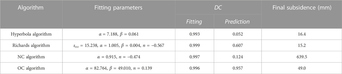
TABLE 4. Algorithm parameters determined based on 256d subsidence monitoring data at section DK 1806 + 925.

TABLE 5

TABLE 5. Algorithm parameters determined based on 256d subsidence monitoring data at section DK 1807 + 250.

FIGURE 7

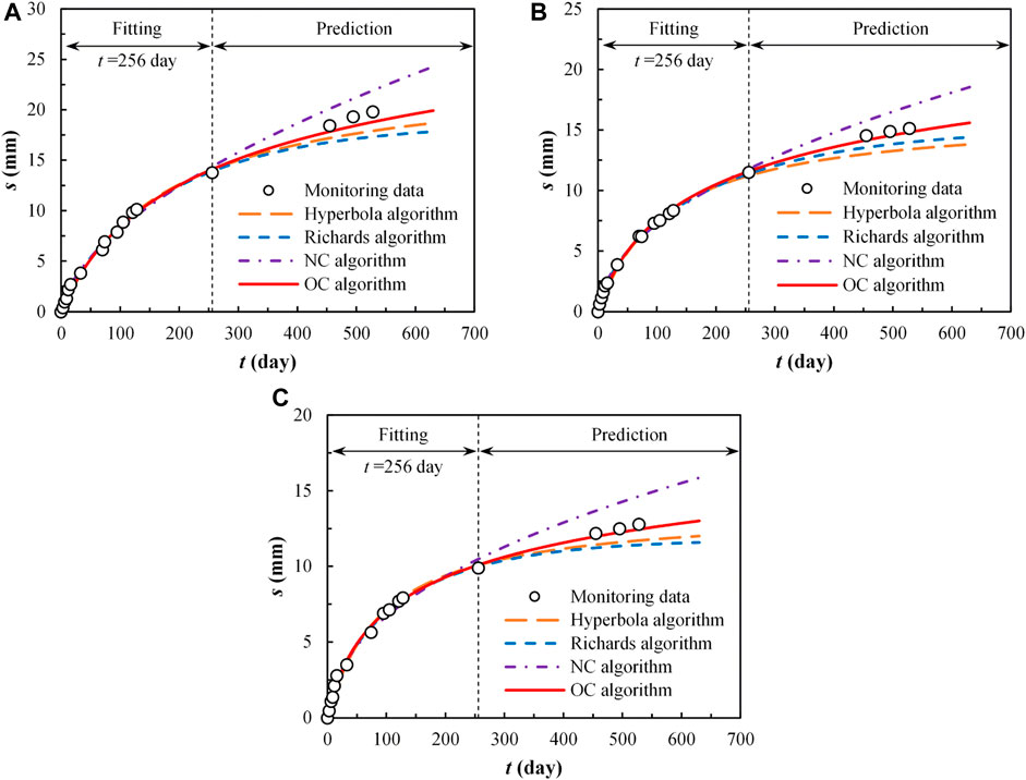
FIGURE 7. Prediction curves for different sections: (A) for section DK 1806 + 800; (B) for section DK 1806 + 925; (C) for section DK 1807 + 250.

According to Figure 7, all the curves fit the monitoring data from days 1–256 well. Combining the values of DC for the prediction stages of each algorithm in Table 3 ∼ 5, the OC algorithm has the best prediction results when predicting the subsidence from days 256–528.

4.3 Analysis and discussion

The prediction results of the Hyperbola algorithm and the Richards algorithm are almost smaller than the subsidence monitoring data from days 256–528. This is similar to the subsidence prediction results of other foundations (Yao et al., 2020). The prediction results of the NC algorithm are obviously larger than the actual subsidence because it regards subgrade soil as normally consolidated soil. In fact, each soil layer must be compacted in the process of subgrade filling, even utilizing dynamic compaction. In this compaction process, part of the subgrade soil has become over-consolidated soil. In addition, subsidence monitoring is generally carried out sometime after the completion of filling. During this time, the subgrade soil has experienced a period of creep. After creep deformation, the void ratio of subgrade soil is smaller, which is equivalent to increasing the over-consolidated ratio. Therefore, the effect of stress history should be considered in subsidence predictions. The OC algorithm regards the subgrade soil as over-consolidated soil and already takes into account the effect of stress history. This is also the reason the OC algorithm has the best prediction results among these four algorithms.

5 Conclusion

Based on the MPF model, this study derives two creep deformation formulas in normal consolidation and over-consolidated state. On this basis, two creep subsidence prediction algorithms are proposed, which consider stress history and do not consider stress history, respectively. The main conclusions can be drawn:

(1) The MPF model is capable of describing the creep properties in one dimension of both fine-grain soil and coarse-grained soil in a uniform manner. At the same time, it also meets the request that the creep deformation grows non-linearly with time to stability. The consolidation test can determine all the parameters of the MPF model.

(2) Based on the MPF model and Bjerrum’s reclassification, and using the INCL in the UH model as the reference line, the MPF model is developed into two creep strain formulas under normal consolidation and over-consolidation conditions. Both formulas satisfy that the creep deformation increases non-linearly from zero to a certain maximum deformation value with time.

(3) Referring to the idea of the layer-wise method, two creep subsidence prediction algorithms considering stress history and without considering stress history are proposed. The parameters of the two prediction algorithms can be obtained through on-site subsidence observation data.

(4) By comparing the fitting results and prediction results with two widely used subsidence prediction algorithms in practical engineering, the proposed prediction algorithm considering stress history has the best prediction results for the subgrade of Haolebaoji-Ji’an Railway because it treats the subgrade soil as over-consolidated soil and already takes into account the effect of stress history.

(5) The prediction algorithm considering stress history provides an efficient tool for calculating creep subsidence of subgrades. However, the applicability of the prediction algorithm for special soils such as expansive soil, wet-collapsible loess, and frozen soil needs further research. In addition, rainfall-induced wetting deformation can also affect the settlement of subgrades. In this case, the applicability of the proposed algorithm also needs to be further researched.

Data availability statement

The raw data supporting the conclusion of this article will be made available by the authors, without undue reservation.

Author contributions

JH: Funding acquisition, Writing–original draft, Writing–review and editing. XL: Writing–original draft, Writing–review and editing. HH: Data curation, Formal Analysis, Writing–review and editing.

Funding

The author(s) declare financial support was received for the research, authorship, and/or publication of this article. This work was supported by the Beijing Postdoctoral Research Foundation of China (Grant No. 2021-zz-106) and the Pyramid Talent Training Project of the Beijing University of Civil Engineering and Architecture (Grant No. JDYC20220813).

Conflict of interest

Author HH was employed by the Company China Construction First Group Corporation Limited.

The remaining authors declare that the research was conducted in the absence of any commercial or financial relationships that could be construed as a potential conflict of interest.

Publisher’s note

All claims expressed in this article are solely those of the authors and do not necessarily represent those of their affiliated organizations, or those of the publisher, the editors and the reviewers. Any product that may be evaluated in this article, or claim that may be made by its manufacturer, is not guaranteed or endorsed by the publisher.

References

Bai, B., Cai, G., Hu, W., Yang, G., and Zhou, R. (2021). Coupled thermo-hydro-mechanical mechanism in view of the soil particle rearrangement of granular thermodynamics. Comput. Geotechnics 137 (8), 104272. doi:10.1016/j.compgeo.2021.104272

CrossRef Full Text | Google Scholar

Bai, B., Li, T., Yang, G. C., and Yang, G. S. (2019). A thermodynamic constitutive model with temperature effect based on particle rearrangement for geomaterials. Mech. Mater. 139, 103180. doi:10.1016/j.mechmat.2019.103180

CrossRef Full Text | Google Scholar

Bi, G., Briaud, J. L., Kharenaghi, M. M., and Sanchez, M. (2019). Power law model to predict creep movement and creep failure. J. Geotechnical Geoenvironmental Eng. 145 (9), 04019044. doi:10.1061/(asce)gt.1943-5606.0002081

CrossRef Full Text | Google Scholar

Bjerrum, L. (1967). Engineering geology of Norwegian normally-consolidated marine clays as related to settlements of buildings. Géotechnique 17 (2), 83–118. doi:10.1680/geot.1967.17.2.83

CrossRef Full Text | Google Scholar

Briaud, J. L., and Garland, E. (1985). Loading rate method for pile response in clay. J. Geotechnical Eng. 111 (3), 319–335. doi:10.1061/(ASCE)0733-9410(1985)111:3(319)

CrossRef Full Text | Google Scholar

Briaud, J. L., and Gibbens, R. (1999). Behavior of five large spread footings in sand. J. Geotechnical Geoenvironmental Eng. 125 (9), 787–796. doi:10.1061/(ASCE)1090-0241(1999)125:9(787)

CrossRef Full Text | Google Scholar

Cheng, Z. L., and Ding, H. S. (2007). Experimental study on engineering characteristics of rockfill materials. Yangtze River 120 (7), 110–114. doi:10.16232/j.cnki.1001-4179.2022.07.035

CrossRef Full Text | Google Scholar

Crawford, C. B. (1964). Interpretation of the consolidation test. J. Soil Mech. Found. Div. 90 (SM5), 87–102. doi:10.1061/JSFEAQ.0000664

CrossRef Full Text | Google Scholar

Degago, S. A., Grimstad, G., Jostad, H. P., Nordal, S., and Olsson, M. (2011). Use and misuse of the isotache concept with respect to creep hypotheses A and B. Géotechnique 61 (10), 897–908. doi:10.1680/geot.9.P.112

CrossRef Full Text | Google Scholar

Feng, T. W. (2010). Some observations on the oedometric consolidation strain rate behaviors of saturated clay. J. Geoengin. 5 (1), 1–7. doi:10.6310/JOG.2010.5(1).1

CrossRef Full Text | Google Scholar

Huang, C. F., Li, J. Y., Li, Q., Wu, S. C., and Xu, X. L. (2018). Application of the Richards model for settlement prediction based on a bidirectional difference-weighted least-squares method. Arabian J. Sci. Eng. 43 (10), 5057–5065. doi:10.1007/s13369-017-2909-0

CrossRef Full Text | Google Scholar

Huang, J., Lu, X. S., Peng, R., Qi, J. L., and Yao, Y. P. (2023). A simplified algorithm for predicting creep settlement of high fills based on modified power law model. Transp. Geotech., 101078. doi:10.1016/j.trgeo.2023.101078

CrossRef Full Text | Google Scholar

Karim, M. R., Gnanendran, C. T., Lo, S. C., and Mak, J. (2010). Predicting the long-term performance of a wide embankment on soft soil using an elastic-viscoplastic model. Can. Geotechnical J. 47 (2), 244–257. doi:10.1139/T09-087

CrossRef Full Text | Google Scholar

Kuwano, R., and Jardine, R. J. (2002). On measuring creep behaviour in granular materials through triaxial testing. Can. Geotechnical J. 39 (5), 1061–1074. doi:10.1139/t02-059

CrossRef Full Text | Google Scholar

Luo, Q., Cheng, M., Wang, T. Fei., and Zhu, J. J. (2020). Three-parameter power function model for prediction of post-construction settlement of medium compressive soil foundation. J. Beijing Jiaot. Univ. 44 (3), 93–100. doi:10.11860/j.jssn.1673-0291.20190078

CrossRef Full Text | Google Scholar

Mei, S. A., Chen, S. S., Zhong, Q. M., and Yan, Z. K. (2018). Parametric model for breaching analysis of earth-rock dam. Adv. Eng. Sci. 50 (02), 60–66. doi:10.15961/j.jsuese.201700828

CrossRef Full Text | Google Scholar

Mesri, G., and Choi, Y. K. (1985). Settlement analysis of embankments on soft clays. J. Geotechnical Eng. 111 (4), 441–464. doi:10.1061/(ASCE)0733-9410(1985)111:4(441)

CrossRef Full Text | Google Scholar

Mesri, G. (2009). Effects of friction and thickness on long-term consolidation behavior of Osaka Bay clays. Soils Found. 49 (5), 823–824. doi:10.3208/sandf.49.823

CrossRef Full Text | Google Scholar

Prakash, K., Murthy, N. S., and Sridharan, A. (1987). Rectangular hyperbola method of consolidation analysis. Géotechnique 37 (3), 355–368. doi:10.1680/geot.1987.37.3.355

CrossRef Full Text | Google Scholar

Stolle, D., Vermeer, P. A., and Bonnier, P. G. (1999). A consolidation model for a creeping clay. Can. Geotechnical J. 36 (4), 754–759. doi:10.1139/t99-034

CrossRef Full Text | Google Scholar

Sun, G., Zhang, Y. Q., Li, H. F., Nie, K., Qi, J., Deng, C., et al. (2016). The research of rockfill creep model and parameters. J. China Inst. Water Resour. Hydropower Res. 14 (2), 115–117. doi:10.13244/j.cnki.jiwhr.2016.02.006

CrossRef Full Text | Google Scholar

Wang, H., Li, L., Li, J. P., and Sun, D. A. (2022). Drained expansion responses of a cylindrical cavity under biaxial in situ stresses: numerical investigation with implementation of anisotropic S-CLAY1 model. Can. Geotechnical J. 60 (2), 198–212. doi:10.1139/cgj-2022-0278

CrossRef Full Text | Google Scholar

Yao, Y. P., and Fang, Y. F. (2019). Negative creep of soils. Can. Geotechnical J. 57 (1), 1–16. doi:10.1139/cgj-2018-0624

CrossRef Full Text | Google Scholar

Yao, Y. P., Huang, J., Wang, N., Luo, T., and Han, L. (2020). Prediction method of creep settlement considering abrupt factors. Transp. Geotech. 22, 100304. doi:10.1016/j.trgeo.2019.100304

CrossRef Full Text | Google Scholar

Yao, Y. P., Kong, L. M., and Hu, J. (2013). An elastic-viscous-plastic model for over-consolidated clays. Sci. China-Technological Sci. 56, 441–457. doi:10.1007/s11431-012-5108-y

CrossRef Full Text | Google Scholar

Yin, J. H. (1999). Non-linear creep of soils in oedometer tests. Géotechnique 49 (5), 699–707. doi:10.1680/geot.1999.49.5.699

CrossRef Full Text | Google Scholar

Zhang, Y. Y., Deng, G., Wen, Y. F., Wang, J. P., Wan, Q. W., and Wang, X. H. (2021). Experimental study on consolidation-rheology characteristics of soil-aggregate mixture materials. J. Hydroelectr. Eng. 40 (2), 187–194. doi:10.11660/slfdxb.20210219

CrossRef Full Text | Google Scholar