Impact of detector-element active-area shape and fill factor on super-resolution

1. Introduction

Image acquisition is subject to a variety of phenomena that cause degradations in the signal. All images are impacted by blurring from the system point spread function (PSF) and noise from a range of sources. Additionally, many imaging systems are designed with focal plane arrays (FPAs) having a pixel pitch (i.e., space between detector elements) that does not meet the Nyquist criterion for sampling with regard to the optical cutoff frequency. Such undersampling may lead to aliasing artifacts and reduced image utility. Designing imaging systems for specific applications entails navigating a complex tradespace and involves balancing factors such as optical resolution, field of view, aliasing, signal-to-noise ratio (SNR), integration time, frame rate, as well as size, weight, and power [1]. Similar considerations are involved in the design of microscopy systems [2]. The inclusion of image processing algorithms, such as super-resolution (SR), can influence the selection of many of these system parameters.

It is the goal of SR processing to restore the blurred, noisy, and undersampled imagery acquired from a given imaging system [3–6]. With multi-frame SR, a sequence of frames with inter-frame motion is used to form the SR image estimate [3–6]. In order to deconvolve the linear blur from the PSF, the PSF must be defined on a sampling grid that meets the Nyquist criterion. SR image restoration, which must occur on this grid, generally requires that the observed imagery be upsampled prior to any deconvolution. Sampling diversity provided by multiple input frames makes this upsampling more accurate than with a single frame. Note that the system PSF generally has two main components: diffraction from the optics [7], and spatial detector integration within each detector element [8, 9]. At the observed resolution, the span of the spatial detector integration will not exceed the pixel pitch. However, on the upsampled SR grid, where the PSF is defined, the spatial integration from each detector can now span multiple high resolution samples. In fact, in many undersampled imaging systems, the spatial detector integration becomes the dominant component of the system PSF [8–11]. Thus, the detector element shape and size (relative to the pixel pitch) can play a significant role in image sampling and SR restoration. Conventional FPAs utilize square detector elements with a nearly 100% fill factor, where fill factor is defined as the fraction of the detector element area that is active in light detection. A large fill factor is generally considered to be desirable because more photons are collected for a given pitch, and this leads to a higher SNR. However, the large active area works against SR image restoration by acting as an additional low pass filter in the overall PSF when modeled on the SR sampling grid [12]. A high fill factor also tends to increase blurring from pixel cross-talk [12, 13].

In this paper, we study the impact of FPA detector-element shape and fill factor on SR image restoration. We provide a detailed modulation transfer function (MTF) analysis along with a number of experimental results with both simulated data and real data from a midwave infrared (MWIR) imaging system. We show that there can be significant advantages to low fill factor detectors, when state-of-the-art SR processing is employed. In particular, our results show that circular active area detectors, with an MTF zero at the optical cutoff frequency, provide some of the best results in our tests. The low fill factor detectors trade signal-to-noise ratio for a more favorable overall system MTF that can be exploited by SR restoration. These results have implications for imaging sensor design for both grayscale and division of FPA sensors (e.g., color, multiband, and polarization) [14–16].

The organization of the remainder of this paper is as follows. The observation model is presented in Section 2. The primary analysis of detector element active area and shape is presented in Section 3. In Section 4, we describe the robust adaptive Wiener filter (AWF) [11] SR method used here. Experimental results are presented in Section 5. These results include a detailed quantitative performance analysis using simulated data, and new video results using a commercial MWIR imaging system with both high and low detector element fill factors. Finally, conclusions are offered in Section 6.

2. Observation Model

The observation model used here is shown in Figure 1. It begins with a continuous-space desired image d(x, y), where x, y are continuous spatial variables. We shall define ideal sampling as sampling at or above the Nyquist rate, relative to the optical cutoff frequency, with no PSF blur (other than an ideal band-limiting filter at the optical cutoff frequency) or noise. The discrete image formed by ideal sampling will be represented using lexicographical notation as the vector z = [z₁, z₂, … z_N]^T. In practice, z is not available. Rather, the observed data include PSF blurring, potentially sub-Nyquist sampling, and noise. Blurring from the system PSF is modeled as

$\begin{array}{cc}f(x,y)=d(x,y)*h(x,y),& (1)\end{array}$

where h(x, y) is the continuous space PSF and * represents linear convolution. Modeling the PSF is addressed in detail in Section 2.1. The nonuniform sampling block produces a set of samples from f (x, y) that may, in general, be nonuniformly distributed spatially. In multiframe SR, these samples are collected from multiple frames and registered onto a common grid. The spatial distribution of these samples will depend on the interframe motion [8]. Let the set of nonuniform sample values be represented in lexicographical notation as f = [f₁, f₂, …, f_M]^T. Note the use of bold formatting for the lexicographical vector f, to distinguish it from the parent continuous-space function f (x, y). Using multiple frames with subpixel interframe motion allows one to obtain a more dense sampling of f (x, y) than may be possible with a single image. The resulting samples may or may not meet the Nyquist criterion. However, unless the interframe motion is carefully controlled, the samples will be nonuniformly distributed. An example of the nonuniform samples resulting from three translationally shifted frames is shown in Figure 2. Here the native detector array is square with a detector pitch of 30 μm.

FIGURE 1

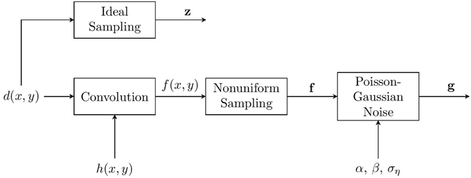
Figure 1. Observation model block diagram.

FIGURE 2

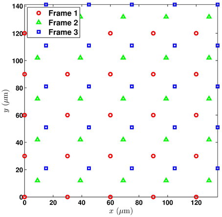
Figure 2. Nonuniform sampling grid composed of the registered collection of three translationally shifted frames, each with a pixel spacing of 30 μm.

The order of operations shown in Figure 1 effectively assumes that the PSF blurring occurs prior to any interframe motion. This is valid for translational interframe motion for any PSF. It is also valid for rotational motion for a circularly symmetric PSF. In the case of modest affine motion and typical PSF parameters, this model holds in an approximate sense, as analyzed in Hardie et al. [10]. The noise in Figure 1 is assumed to be Poisson-Gaussian noise, with both a signal-dependent and signal-independent component [17, 18]. Incorporating the noise gives rise to the observed pixels, denoted g = [g₁, g₂, … g_M]^T. The details of the noise model are desribed in Section 2.2. The SR restoration problem is to estimate z from the observed g. This inverse problem requires deconvolving h(x, y), and addressing noise and nonuniform sampling. The approach taken by nonuniform-interpolation based SR methods is to estimate a uniform set of samples of f (x, y) from g, and then apply some form of image restoration to deconvolve the PSF blur and reduce noise [3]. Note that the AWF SR method that we employ here performs this nonuniform interpolation and restoration in a single weighted sum operation [8]. However, the main focus of this paper is not on the internal workings of any specific SR method, but rather on the imaging sensor used to acquire the data. In particular, our focus is on the detector element active area size and shape and its impact on the overall MTF and SR results.

2.1. PSF Model

A critical component of the observation model is the PSF, and its Fourier transform, the optical transfer function (OTF) [1]. For this, we shall follow the approach in Hardie [8], Hardie et al. [16], Hardie et al. [10] and model diffraction limited optics and blurring from the spatial integration of the detector elements. In this case, the overall OTF is given by

$\begin{array}{cc}H(u,v)=H_{\text{dif}}(u,v)H_{\det }(u,v),& (2)\end{array}$

where u and v are the horizontal and vertical spatial frequencies in cycles per millimeter, H_dif(u, v) is the OTF from the diffraction-limited optics, and detector integration is modeled with H_det(u, v). For a circular pupil function we have [7]

$\begin{array}{cc}{H}_{\text{dif}}(u,v)=\{\begin{array}{cc}\frac{2}{\pi }\left[{\cos }^{-1}\left(\omega \right)-\omega \sqrt{1-{\omega }^2}\right]& \omega <1\\ 0& \text{else}\end{array},& (3)\end{array}$

where $\omega =\sqrt{u^2+v^2}/{\omega }_c$, the optical cutoff frequency is ω_c = 1/(λF), and F is the f-number of the optics. Note that f-number is defined as the ratio of the focal length of the optics to the effective aperture [1]. The wavelength of light is represented by λ. An example of H_dif(u, v) is shown in Figure 3 for a MWIR imaging system with F = 3.33 and λ = 4.5 μm. Note that this is a bandlimiting OTF with cutoff given by ω_c = 66.66 cycles/mm. The detector OTF, H_det(u, v), is determined by the active area of a single detector on the FPA. More will be said about this in Section 3.

FIGURE 3

Figure 3. Diffraction OTF, H_dif(u, v), for MWIR system with F = 3.33 and λ = 4.5 μm.

Let us define the detector pitch of a native sensor to be p mm. The sampling frequency associated with this sensor is then given by 1/p cycles/mm. To guarantee the absence of aliasing, the Nyquist theorem requires that 1/p > 2ω_c = 2/(λF), or equivalently p < λF/2. Because of the complex tradespace associated with imaging systems design, the pitch in most imaging systems does not meet this requirement. To characterize the level of undersampling in an imaging system, we shall use the parameter Q = λF/p [19]. Note that the undersampling factor is given by 2/Q, such that Q = 2 corresponds to a Nyquist sampled system, and Q = 1 corresponds to a system undersampled by a factor of 2. Note that many imaging systems are designed for Q ≈ 1, as this tends to be a good compromise between aliasing and other factors, such as signal-to-noise ratio [19]. This level of undersampling provides the opportunity for a significant resolution boost using SR post processing. Figure 4 shows how the pitch p and the f-number impact the Q-value for a MWIR imaging system with center wavelength of λ = 4.5 μm.

FIGURE 4

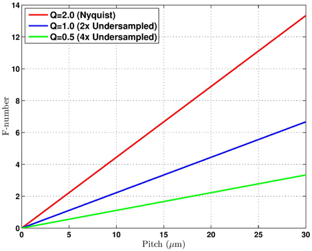
Figure 4. Sampling relationship between pitch and f-number for λ = 4.5 μm. Three Q-values curves are shown where Q = λF/p.

Now consider Equation (2) in the spatial domain. The continuous-space system PSF is given by

$\begin{array}{cc}h(x,y)=\text{ICSFT}\{H(u,v)\}=h_{\text{dif}}(x,y)*h_{\det }(x,y),& (4)\end{array}$

where h_dif(x, y) is the diffraction PSF, h_det(x, y) is the PSF associated with the detector, and ICSFT{·} is the inverse continuous-space Fourier transform. We may define a valid impulse-invariant discrete-space PSF, h_ii(n₁, n₂) by sampling h(x, y) at or above the Nyquist rate. This gives

$\begin{array}{cc}{h}_{ii}(n_1,n_2)={\Delta }_x{\Delta }_{y}h(n_1{\Delta }_x,n_2{\Delta }_y),& (5)\end{array}$

where Δ_x, Δ_y < λF/2. We approximate this discrete PSF directly using the frequency sampling filter design method based on the analytic expression for the OTF in Equation (2) and Nyquist rate sample spacings of Δ_x, Δ_y. With this discrete PSF, we are able to accurately model the continuous PSF blurring using discrete convolution. Furthermore, the discrete PSF is used to design the AWF SR restoration filters.

2.2. Noise Model

Consider a Poisson-Gaussian noise model that accounts for the photon arrival distribution as well as noise in the electronics [17, 18]. Applying this model, the observed data are given by

$\begin{array}{cc}g=\alpha p+\beta 1+\eta ,& (6)\end{array}$

where p ~ P((f − β1)/α) is an iid Poisson random vector with mean of (f − β1)/α. The random vector p models the observed signal in the presence of shot noise, prior to any camera gain or offset. The parameter α is a camera gain, β is a camera offset, and 1 is an M × 1 vector of ones. Since the variance of a Poisson random variable equals its mean, the covariance matrix of p is given by $P=\text{diag}\left(\frac{f_1-\beta }{\alpha },\frac{f_2-\beta }{\alpha },\dots ,\frac{f_M-\beta }{\alpha }\right)$. The vector η ~ N(0, σ²_ηI) is an iid Gaussian random vector modeling the electronics noise terms. Note that the mean of g in Equation (6) is f, and the covariance is given by G = α² P + σ²_ηI. Also, note that G is diagonal and the i'th diagonal element is given by α(f_i − β) + σ²_η. For high mean values, a Poisson distribution is known to be well approximated by a Gaussian. In this case, we can approximate g as a heteroskedastic Gaussian random vector, such that g ~ N(f, G) [17, 18]. This is equivalent to an additive Gaussian noise with a signal dependent variance, given by g = f + n, where n ~ N(0, G). For generating all of the simulated data in Section 5, we will use the noise model in Equation (6). However, the AWF SR algorithm is based on additive signal independent noise. For the purposes of AWF SR processing we shall assume the heteroskedastic model and use constant noise variance of σ²_n = α(f − β) + σ²_η, where f = E{f_i}.

Now, consider the impact of a changing signal level on this Poisson-Gaussian noise. In particular, let the incoming signal be scaled by s as a result of integration time change or ambient signal level changes. The noise variance associated with the average scaled signal level is σ²_n(s) = α(sf − β) + σ²_η. However, a gain of 1/s is needed to bring this scaled image back to the original level for comparison. Thus, the effective noise level of the scaled signal, relative to the s = 1 system, is

$\begin{array}{cc}{\sigma }_e^2(s)=\frac{1}{s^2}{\sigma }_n^2(s)=\alpha \left(\frac{1}{s}\overline{f}-\frac{1}{s^2}\beta \right)+\frac{1}{s^2}{\sigma }_{\eta }^2.& (7)\end{array}$

If β = 0, which is the case for most cameras, we get the following relationship

$\begin{array}{cc}{\sigma }_e^2(s)=\frac{1}{s}\alpha \overline{f}+\frac{1}{s^2}{\sigma }_{\eta }^2.& (8)\end{array}$

Thus, we see that the noise variance due to the signal dependent Poisson component scales with 1/s, while the signal-independent additive Gaussian noise component scales with 1/s². This has important ramifications for the detector active area analysis. A photon limited system, with very low σ²_η, will have a 1/s increase in noise from a reduced signal level (i.e., s < 1) that might come from a reduced detector active area. However, a system dominated by thermal noise will have a 1/s² increase in effective noise. For the simulation results in Section 5.1, we shall use 8 bit image data to represent the true scene. Thus, we use camera model parameters typical of commercial cameras operating in an 8 bit dynamic range, that is 0–255 digital units (DUs). The parameters we use are α = 0.02, β = 0.00, and σ²_η = 0.50. This gives us the effective noise variance relationship shown in Figure 5, based on Equation (8).

FIGURE 5

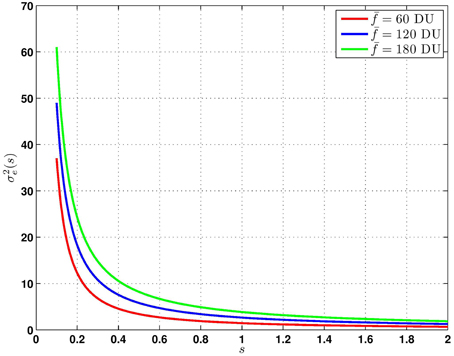
Figure 5. Effective noise variance, σ²_e(s), as a function of signal scaling s, for three values of f for α = 0.02, β = 0.00, and σ²_η = 0.50.

3. Analysis of Detector Shape

In this section, we focus on how the detector active area shape impacts the overall system PSF and OTF. We first show exactly how the detector PSF model relates to the active area of an element of an FPA in Section 3.1. Next, in Section 3.2, we examine rectangular and circular active area detectors. In Section 3.3, we provide a detailed system MTF analysis by combining the diffraction and detector components of the MTF model. Finally, in Section 3.4, we examine variable response detectors and their MTFs.

3.1. Detector PSF

Consider the image on the focal plane resulting from diffraction limited optics with no spatial integration from the detector elements. This image is given by

$\begin{array}{cc}\overline{d}(x,y)=d(x,y)*h_{\text{dif}}(x,y).& (9)\end{array}$

If we define the active area of a single detector element centered at (0, 0) as a(x, y), then we have

$\begin{array}{cc}{f}_i={\displaystyle \underset{{\tau }_1=-\infty }{\overset{\infty }{\int }}{\displaystyle \underset{{\tau }_2=-\infty }{\overset{\infty }{\int }}\overline{d}({\tau }_1,{\tau }_2)a({\tau }_1-x_i,{\tau }_2-y_i)d{\tau }_{1}d{\tau }_2}},& (10)\end{array}$

for i = 1, 2, …, M, where x_i, y_i are the spatial coordinates of the detector element for sample i. This models the spatial integration associated with the detector active area. Allowing for a continuum of detector positions, we obtain

$\begin{array}{cc}f(x,y)={\displaystyle \underset{{\tau }_1=-\infty }{\overset{\infty }{\int }}{\displaystyle \underset{{\tau }_2=-\infty }{\overset{\infty }{\int }}\overline{d}({\tau }_1,{\tau }_2)a({\tau }_1-x,{\tau }_2-y)d{\tau }_{1}d{\tau }_2}}.& (11)\end{array}$

This represents a deterministic correlation operation between d(x, y) and a(x, y). If we define h_det(x, y) = a(−x, −y), then we have

$\begin{array}{cc}f(x,y)={\displaystyle \underset{{\tau }_1=-\infty }{\overset{\infty }{\int }}{\displaystyle \underset{{\tau }_2=-\infty }{\overset{\infty }{\int }}\overline{d}({\tau }_1,{\tau }_2)h_{\det }(x-{\tau }_1,y-{\tau }_2)d{\tau }_{1}d{\tau }_2}}.& (12)\end{array}$

Note that this equivalent to the convolution operation f (x, y) = d(x, y) * h_det(x, y). Thus, the detector PSF is simply a reflected version of the active area, h_det(x, y) = a(−x, −y). If the active area is symmetric, then we have h_det(x, y) = a(x, y).

3.2. Rectangular and Circular Detectors

We focus on two basic active area shapes, rectangular and circular. Figure 6 shows representations of FPAs with rectangular and circular detector active areas. The detector spacings, or pitches, are given by p₁ and p₂ in the horizontal and vertical dimensions, respectively. For the rectangular detectors shown in Figure 6 (left), we have

$\begin{array}{cc}{h}_{\det }(x,y)=\text{rect}\left(\frac{x}{a_1},\frac{y}{a_2}\right),& (13)\end{array}$

where

$\begin{array}{cc}\text{rect}(x,y)=\{\begin{array}{cc}1& \left|x\right|,\left|y\right|<0.5\\ 0& \text{otherwise}\end{array}.& (14)\end{array}$

FIGURE 6

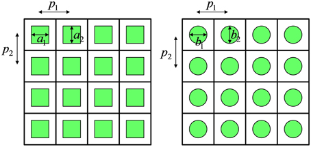
Figure 6. Representation of FPAs with rectangular (left) and circular (right) active area detector elements.

The spatial frequency response associated with this detector shape is given by the CSFT such that

$\begin{array}{cc}{H}_{\det }(u,v)=\text{CSFT}\{h_{\det }(x,y)\}=a_1{a}_2·\text{sinc}\left(a_{1}u,a_{2}v\right),& (15)\end{array}$

where

$\begin{array}{cc}\text{sinc}(u,v)=\frac{\sin (\pi u)\sin (\pi v)}{(\pi u)(\pi v)}.& (16)\end{array}$

The detector MTF for a square detector element with a = a₁ = a₂ = 30 μm is shown in Figure 7. Note that in general, the spatial frequency response in Equation (15) has zeros every integer multiple of 1/a₁ in u, and 1/a₂ in v. We shall see that these zeros are particularly consequential when performing SR on an upsampled grid (i.e., sample spacing less than p₁, p₂). Consider a square sampling FPA with p = p₁ = p₂. For a 100% fill factor detector (i.e., a = a₁ = a₂ = p), the zeros occur at integer multiples of 1/p in u and v. The optical cutoff frequency can be expressed in terms of Q as ω_c = 1/(pQ). Thus, for a system with Q < 1, the 100% fill factor detectors put a zero within the spatial frequency pass band of the diffraction limited optics OTF. This means that spatial frequency information that is potentially restorable via SR, would be completely eliminated. If instead of 100% fill factor, we set a = a₁ = a₂ = pQ for systems with Q < 1, the detector zero will occur at the optical cutoff frequency, preventing a detector zero from entering the diffraction OTF pass band. Thus, systems with Q < 1 may benefit from a reduced fill factor detector (i.e., a < p) to move the detector zero out toward or beyond the optical cutoff frequency. It should be noted that systems with a low Q also have the most to gain from SR because of the high level of undersampling.

FIGURE 7

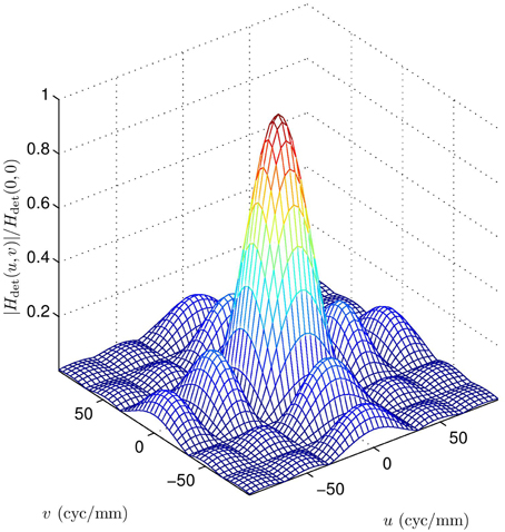
Figure 7. Square detector MTF for detector element width a = a₁ = a₂ = 30 μm.

For the circular detectors, shown in Figure 6 (right), we have

$\begin{array}{cc}{h}_{\det }(x,y)=\text{circ}\left(\frac{x}{b_1},\frac{y}{b_2}\right),& (17)\end{array}$

where

$\begin{array}{cc}\text{circ}(x,y)=\{\begin{array}{cc}1& \sqrt{x^2+y^2}<0.5\\ 0& \text{otherwise}\end{array}.& (18)\end{array}$

The spatial frequency response associated with the circular detector shape is

$\begin{array}{cc}{H}_{\det }(u,v)=\text{CSFT}\{h_{\det }(x,y)\}=b_1{b}_2·\text{jinc}\left(b_{1}u,b_{2}v\right),& (19)\end{array}$

where

$\begin{array}{cc}\text{jinc}(u,v)=J_1\left(\pi \omega )/(2\omega \right),& (20)\end{array}$

$\omega =\sqrt{u^2+v^2}$, and J₁ is an order one Bessel function of the first kind. The zeros of this frequency response do not occur at regular intervals like the rect function. However, the very important first zero occurs at approximately 1.22/b₁ on the u axis and approximately 1.22/b₂ on the v axis. To align the circular detector first zero with the optical cutoff frequency for the case of a square grid of pitch p, we require b = b₁ = b₂ = 1.22pQ. The detector MTF for a circular detector element with b = b₁ = b₂ = 30 μm is shown in Figure 8.

FIGURE 8

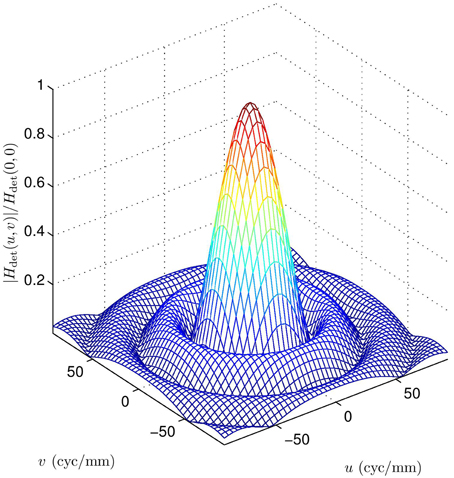
Figure 8. Circular detector MTF for detector element diameter b = b₁ = b₂ = 30 μm.

In division of FPA sensors like Bayer pattern color sensors, multiband, and polarimetric imagers, a single FPA uses detector elements of different types in alternating patterns. An example of a polarimetric division of FPA array is shown in Figure 9 [14, 16]. Thus, the active area of a given detector element type must be less than the pitch between like-elements (to make room for the other element types). It is interesting to note that this naturally gives the kind of reduced active area discussed above. If the system is designed for a Q = 0.5 for one channel, and the patterns is like that shown in Figure 9, then the active area for each channel is the prescribed a = a₁ = a₂ = pQ when using the full FPA area. Thus, if one does wish to employ reduced active area detectors for enhanced MTF purposes, the “lost” area can be put to good use by employing a division of FPA design [14, 16]. Another good use for the “lost” active area is to serve as a guard band to greatly reduce diffusion of charge carriers from one detector element to the other. Such diffusion leads to parasitic low pass spatial filtering of the imagery, causing an additional loss of resolution [12].

FIGURE 9

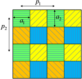
Figure 9. Example of a division of FPA detector array with four polarimetric channels.

3.3. MTF Analysis

The overall MTF, combining diffraction and detector integration, is shown in Figure 10 for the case of F = 3.33, λ = 4.5 μm, and a = a₁ = a₂ = 30 μm. Note that the first zeros from the detector MTF impact the overall MTF within the spatial frequency passband of the optics. A cross section of this MTF and component MTFs is shown in Figure 11. For a detector pitch of 30 μm (i.e., 100% fill factor), this system would have a native Q = 0.5. The folding frequency (i.e., one half of the sampling frequency) is shown on Figure 11 along with the SR folding frequency for an upsampling factor of L = 4. Notice how the detector MTF zero is right in the middle of the diffraction MTF pass band. Without SR processing, this zero would be above the folding frequency and would be in the band of aliased frequencies. Thus, the lost information from the zero would not be consequential. However, if SR is being performed and we are seeking to recover valid spatial frequency content out to the SR folding frequency, the detector zero is highly undesirable. Similar plots are shown in Figures 12, 13 and Video 2.MOV, but for 25% fill factor square detectors with a = a₁ = a₂ = 15 μm. Note that here the detector zero aligns with the optical cutoff frequency, allowing for the potential recovery of all spatial frequencies afforded by the optics.

FIGURE 10

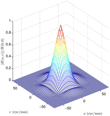
Figure 10. Overall system MTF for the diffraction OTF in Figure 3 (F = 3.33, λ = 4.5 μm), and the detector MTF in Figure 7 (square with a = 30 μm). Note the zeros from the detector impact the overall MTF within the spatial frequency passband of the optics.

FIGURE 11

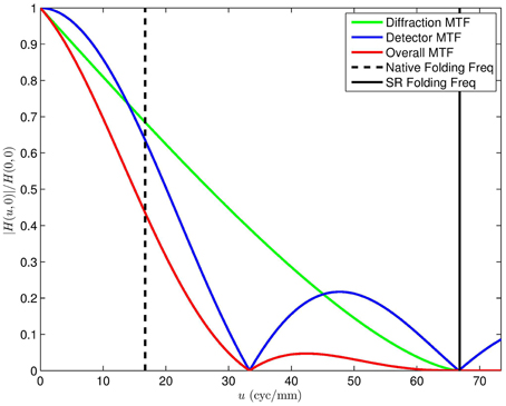
Figure 11. Cross section of the MTF for Figure 10. The diffraction and detector component of the overall MTF can be clearly seen. The native folding frequency for p = 30 μm (100% fill factor, Q = 0.5), is shown along with the L = 4 SR folding frequency.

FIGURE 12

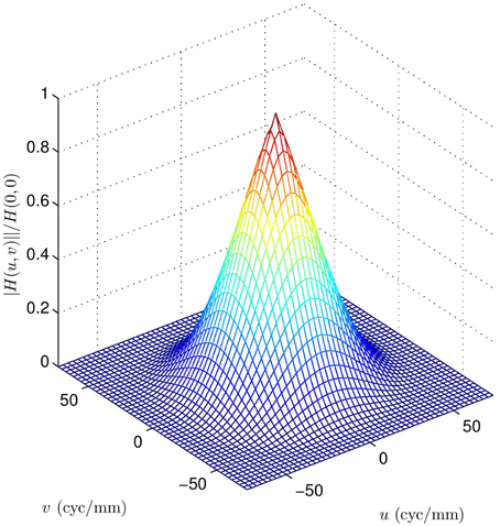
Figure 12. Overall system MTF for the diffraction OTF in Figure 3 (F = 3.33, λ = 4.5 μm), and a square detector MTF with a = 15 μm (i.e., 25% fill factor). Note the zero from the detector does not impact the overall MTF within the spatial frequency passband of the optics.

FIGURE 13

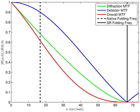
Figure 13. Cross section of the MTF for Figure 12. The native folding frequency for p = 30 μm is shown along with the L = 4 SR folding frequency.

It is important to note that the MTFs are normalized to have a peak value of 1. While the curves in Figures 10–13 clearly show how the detector zero changes, the reduction in signal level from the reduced fill factor is not shown. Note that the signal level is proportional to the active area, and signal gain is reduced when decreasing active area. Therefore, the big question is this: is the loss in overall signal level justified by a favorable detector zero location? To help answer this question, consider the plot in Figure 14. This shows the relative gain as the detector zero is moved from 1/p cycles/mm (for a 100% fill factor) to 1/pQ cycles/mm (where the first detector zero is aligned with the optical cutoff frequency). The red curve on the bottom is for a square detector, and the blue curve on top is for a circular detector. This shows the reduction in signal as the active area is reduced and the detector zero is pushed toward the optical cutoff frequency. It also shows that the circular detector is more efficient than the rectangular one in this regard. The circular detector provides more signal for a given zero location. Note that the relative gain, designated G here, can be thought of as the factor s is Equation (8), with direct consequences on the effective noise variance and SNR.

FIGURE 14

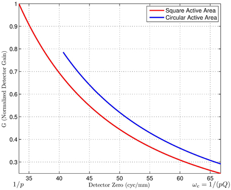
Figure 14. Detector integration gain vs. the detector zero frequency. The gain plotted relative to a 100% fill factor detector with a = 30 μm having a zero at ω = 1/p. Note that to move the detector zero out toward the optical cutoff frequency, a and b must be decreased for rectangular and circular detectors, respectively. The resulting reduction in fill factor causes a lowering of the gain. Interestingly, the circular detector can achieve the higher detector zero with a somewhat larger area.

When the gain is incorporated with the MTF, we get the scaled MTFs shown in Figure 15 and Video 3.MOV. The 100% fill factor MTF is normalized to 1. The scaled MTFs for reduced fill factor detectors are also shown for direct comparison. Note that the loss of signal is seen as a global scaling, reducing the MTFs relative to the 100% fill factor configuration. However, the reduced fill factor architectures do not have the zero at 33.33 cycles/mm. It should be noted that a reduction in gain is quite different than a complete signal loss. Conventional signal processing has no reliable means to recover lost frequency components. However, attenuated spatial frequency content can be amplified with techniques such as Wiener filtering. Thus, we argue that the reduction in signal gain is justified by the potential to recover all spatial frequency components below the optical cutoff frequency. A similar plot to that in Figure 15 is shown Figure 16, but for F = 4, Q = 0.6, and SR upsampling of L = 3. This additional plot is shown because it matches the MWIR systems used in the experimental results in Section 5.2. Because Q is slightly higher in Figure 16, the detector zero is moved less to reach the optical cutoff frequency. This means we have somewhat larger active area detectors and less signal attenuation. Of course, we still have the advantage of no detector zeros below SR folding frequency and optical cutoff frequency.

FIGURE 15

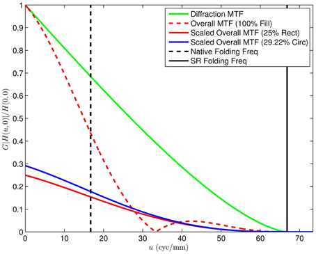
Figure 15. Cross-section of the MTF for Figure 12 scaled by the detector Gain from Figure 14. Here one can compare the overall system MTF employing a 100% fill factor with a gain adjusted MTF for the systems with the detector zeros shifted out to the optical cutoff frequency. Note that even though the gain is much lower, the overall transfer function for the frequency band between 30 and 40 cyc/mm is higher using the smaller detectors, because of the detector zero.

FIGURE 16

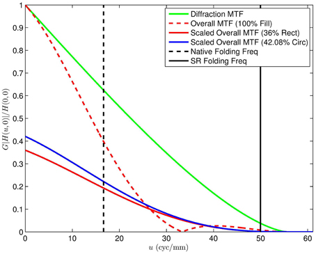
Figure 16. Cross-section MTF plot similar to that in Figure 15, except here we have an f-number of F = 4 (Q = 0.6) and L = 3 for SR. This represents the set up for the experimental results for the infrared imaging system in Section 5.2.

To illustrate how the detector active areas need to be altered to match the detector zero to the optical cutoff frequency, we have included a number of cases in Table 1. This table shows a set of MWIR imaging system parameters for a pitch of p = 30 μm, λ = 4.5 μm, and a variety of f-numbers. Note that as f-number goes down, the optical cutoff frequency goes up. For a fixed p = 30 μm, this means the undersampling goes up. To make the first detector zero align with the increasing optical cutoff frequency requires decreasing a for the square active area detectors and decreasing b for the circular active area detectors. In particular, we require that a = pQ and b = 1.22pQ, as described in Section 3.2. The reduction of a and b creates a lower fill factor, and lower relative signal gain. However, with the smaller active area systems, we do not have a detector zero in the middle of the optical pass band. Note that the fill factor for the circular detector is larger than that of the corresponding square detector by a factor of 1.22²π/4. For example, consider Row 4 in Table 1. With Q = 0.5, the rectangular detector fill factor is 25% and the circular fill factor is 29.22%. Since b cannot be larger than p on single FPA, we do not show values for the circular detector for Q = 0.90 and 1.00.

TABLE 1

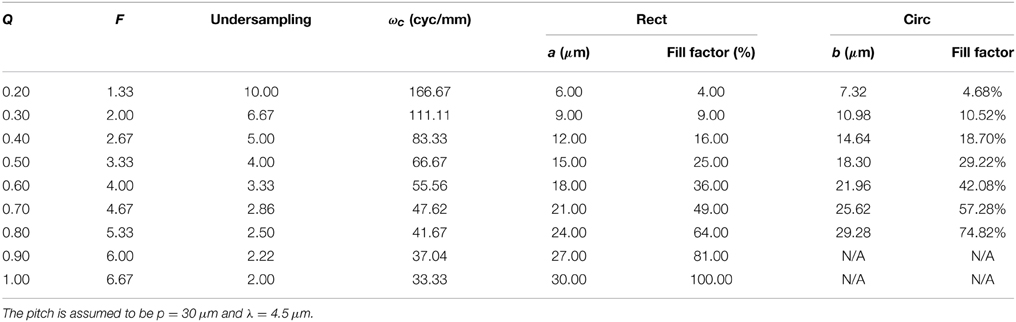
Table 1. Imaging system parameters where a and b are sized so as to produce their first MTF zero at the optical cutoff frequency, ω_c.

3.4. Variable Response Detectors

In addition to active areas that are binary, we also consider variable response active area detectors. Note that these are akin to signal window functions, in that they must taper from zero to some maximum sensitivity and back to zero in a finite length (in this case p = 30 μm). Cross-sections of the window functions considered are shown in Figure 17. Cross-sections of the detector MTFs corresponding to 2D separable versions of the shapes in Figure 17 are shown in Figure 18. Cross-sections of the detector MTFs corresponding to 2D circularly symmetric versions of the shapes in Figure 17 are shown in Figure 19. The conclusion we reach from this analysis is that the variable response detectors do not appear to provide more favorable MTF's than the simple binary versions. Furthermore, they would undoubtedly come with significant manufacturing challenges, and would not be as suitable for division of FPA sensors as their binary counterparts.

FIGURE 17

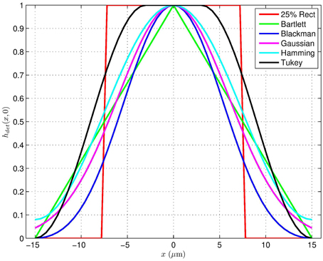
Figure 17. Cross-sections of separable active areas for a pitch of p = 30 μm based on standard window functions. These correspond to variable response detectors, in contrast with binary active area detectors.

FIGURE 18

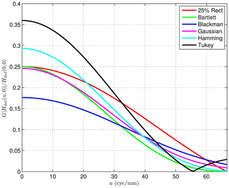
Figure 18. Detector magnitude frequency response of the separable active areas in Figure 17 scaled relative to the DC gain of a 100% fill factor detector.

FIGURE 19

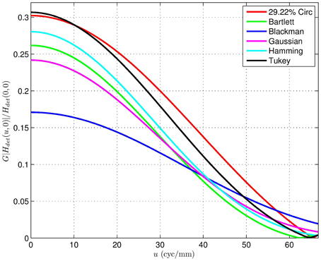
Figure 19. Detector magnitude frequency response of circularly symmetric versions of the active areas in Figure 17 scaled relative to the DC gain of a 100% fill factor detector.

4. Super-Resolution

For the results presented here, we employ the robust AWF SR method proposed in [11] which is based on that in Hardie [8], Hardie [20]. A brief review of that method is provided here for the reader's convenience. The basic methodology is shown in Figure 20. The output high resolution (HR) image, relative to a low-resolution (LR) frame, is increased by a factor of L in both the horizontal and vertical dimensions. We use a moving temporal window of K frames to estimate each output frame. Global registration that is robust to small amounts of local motion is employed to get precise subpixel registration parameters for the bulk of the imagery. Local motion is detected based on an inconsistency with the estimated global motion parameters. In particular, we register the K frames globally, apply a low pass filter to attenuate aliasing artifacts and noise, and then we compute the temporal range at each pixel. Thresholding is used to detect large variations at a given spatial location. The pixel in these areas are labeled as invalid because accurate registration is not available [11]. Note that the most recent frame is designated as the reference frame and all pixels from the reference frame are labeled as valid.

FIGURE 20

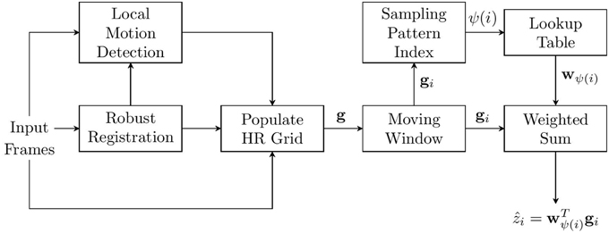
Figure 20. Robust AWF SR. A weighted sum of sampled from all registered frames are used for each observation window. In areas where local motion is detected, only samples from the reference frame are used.

Given the registration information as well as the local pixel labels, the samples from all K frames are placed on a common HR grid. A moving window centered about HR output pixel i is used and the valid sampled spanned by this window are placed into the observation vector g_i = [g_{i, 1}, g_{i, 2}, …, g_{i, Gi}]^T. The AWF SR output is given by

$\begin{array}{cc}{\widehat{z}}_i=w_{\psi (i)}^T{g}_i,& (21)\end{array}$

for i = 1, 2, …, N, where ẑ_i is the estimate of the i'th pixel in z. The parameter ψ(i) is the population index for window i. This is an integer that uniquely specifies the spatial pattern of observed valid pixels for the given observation window position. The AWF filter weights for the particular population index are specified in w_ψ(i) = [w_{ψ(i), 1}, w_{ψ(i), 2}, …, w_{ψ(i), Gi}]^T.

The minimum mean squared error (MSE) Wiener weights are used for the AWF method [8, 11]. These are given by

$\begin{array}{cc}{w}_{\psi (i)}=R_{\psi (i)}^{-1}{p}_{\psi (i)},& (22)\end{array}$

where R_ψ(i) = E{g_ig^T_i|Ψ = ψ(i)} is the autocorrelation matrix, p_ψ(i) = E{z_ig_i|Ψ = ψ(i)} is the cross-correlation vector, and Ψ is a random variable representing the population index. The correlations are found based on a parametric model that considers the distances between all of the samples in each observation window and the distances of these samples to the desired HR pixel. The correlations are based on an assumed autocorrelation function for d(x, y), which is given by

$\begin{array}{cc}{r}_{dd}(x,y)={\sigma }_d^2{\rho }^{\sqrt{x^2+y^2}},& (23)\end{array}$

where x and y are continuous spatial coordinates measured in HR pixel spacings, σ²_d is the variance of the desired signal, and ρ is the one HR pixel step correlation value. Using the observation model in Figure 1, it can be shown that the cross-correlation function between d(x, y) and f (x, y), can be expressed in terms of r_dd(x, y) [8] as

$\begin{array}{cc}{r}_{df}(x,y)=r_{dd}(x,y)*h(x,y).& (24)\end{array}$

Similarly, the autocorrelation of f (x, y) is given by

$\begin{array}{cc}{r}_{ff}(x,y)=r_{dd}(x,y)*h(x,y)*h(-x,-y).& (25)\end{array}$

Sampling the autocorrelation function in Equation (25) at x, y values corresponding to the displacement between samples in g_i yields E{f_if^T_i|Ψ = ψ(i)}, where f_i is the noise-free version of g_i. In the case of independent additive white Gaussian noise of variance σ²_n, it is straightforward to show that R_ψ(i) = E{f_i f^T_i|Ψ = ψ(i)} + σ²_nI. A similar apporach used to obtain the needed p_ψ(i). Here we evaluate Equation (24) based on the displacements between the samples in g_i and z_i.

In this paper we consider translational interframe motion. In areas with no local motion, the sampling pattern on the HR grid is therefore periodic. This means that a relatively small number of unique population patterns are observed. Thus, we can easily precompute the weights and use a lookup table, as shown in Figure 20, to allow for fast processing [8]. Where local motion impacts an observation window, we weight only the reference frame samples, giving a single frame AWF estimate in those areas. This allows for fast processing, even in the presence of some local motion.

One key thing to note here is that the system PSF, h(x, y), governs the statistics used to form the weights. Thus, the detector element model that impacts h(x, y), impacts the AWF SR weights. In practice the correlations in Equations (24) and (25) are evaluated on a high resolution discrete grid using an impulse invariant version of the systems PSF and a sampled version of Equation (23). The correlation values for any x, y values are obtained by interpolating these discrete correlation signals.

5. Experimental Results

In this section, we present results using simulated data for quantitative performance analysis. We also present results using real data from a MWIR imaging system.

5.1. Simulated Data

For the simulations, we use a grayscale chirp image and 8 uncompressed images from the Kodak lossless true color image suite [21]. The Kodak images have been converted to grayscale for our purposes. All of the original images are 8 bit grayscale images. All of the simulation results are based on the observation model with F = 3.33, Q = 0.5, λ = 4.5 μm, and p = 30 μm (i.e., the 4th row in Table 1). The noise comes from the Poisson-Gaussian noise model with α = 0.02, β = 0.00, and σ²_η = 0.50. The SR processing uses K = 16 frames with L = 4 and assumes noise of σ²_n = α (f − β) + σ²_η.

The first image results are for a region of interest (ROI) from the full chirp image and are shown in Figure 21. The high resolution truth image is shown in Figure 21F. The average value for simulated 100% fill factor detectors is f = 127.4 (σ_n = 1.75 DU). Bicubic interpolation images from a single low resolution noisy frame generated with 100% fill factor (a = 30 μm) and 25% fill factor (a = 15 μm) are shown in Figures 21A,B, respectively. Notice the extra aliasing artifacts in the low fill factor detector image, especially near the perimeter of the outer circle. Also notice the increase in effective noise (lower SNR). The outputs of AWF SR using 100% and 25% fill factor input images are shown in Figures 21C,D, respectively. Notice the aliasing is greatly reduced in both images due to the SR processing. However, the image obtained from the 25% fill factor images shows increased high spatial frequency content. Finally, the AWF SR output using simulated circular detectors with 29.22% fill factor (b = 18.3 μm) is shown in Figure 21E. This result is very similar to that obtained with the reduced fill factor square detectors, although there is slightly less noise with the circular detectors. Note that the fill factors for the 25% rectangular detector and the 29.22% circular detector were were chosen so that the first detector MTF zero is located at the optical cutoff frequency for both.

FIGURE 21

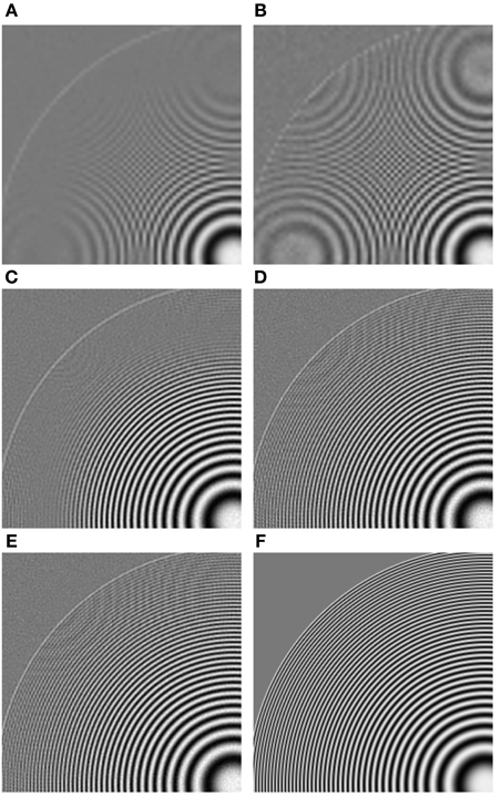
Figure 21. AWF SR results for the 8 bit chirp image using simulated MWIR system with Q = 0.50 from Table 1 with K = 16 frames and L = 4.(A) Bicubic interpolation of a single frame with 100% fill factor detectors (a = 30 μm); (B) bicubic interpolation of a single frame with 25% fill factor square detectors (a = 15 μm); (C) AWF SR using 100% fill factor detectors; (D) AWF SR using 25% fill square factor detectors; (E) AWF SR using 29.22% fill circular detectors (b = 18.3 μm); (F) truth image.

A similar set of results is shown in Figure 22 for a natural image of a motocross scene (kodim05.png). Here, f = 82.65 for the 100% fill factor image (σ_n = 1.47 DU). The truth image is shown in Figure 22F. As with the chirp image, note the increased aliasing using the low fill factor detector in Figure 22B compared with 100% fill factor in Figure 22A. Also note the note the improvement in the AWF SR image using the low fill factor detector in Figure 22D compared with Figure 22C. In particular, notice the detail on the front fork shock absorber cover in the center of the image for the 25% fill factor image that is not present with the 100% fill factor. As with the chirp result, the circular detector image in Figure 22E is very similar to the reduced fill factor square detector image, but with a very slight reduction in noise.

FIGURE 22

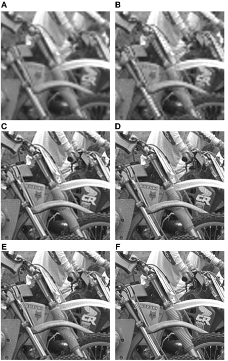
Figure 22. AWF SR results for the 8 bit motocross image (kodim05.png) using simulated MWIR system with Q = 0.50 from Table 1 with K = 16 frames and L = 4. (A) Bicubic interpolation of a single frame with 100% fill factor detectors (a = 30 μm); (B) bicubic interpolation of a single frame with 25% fill factor square detectors (a = 15 μm); (C) AWF SR using 100% fill factor detectors; (D) AWF SR using 25% fill square factor detectors; (E) AWF SR using 29.22% fill circular detectors (b = 18.3 μm); (F) truth image.

To illustrate the impact of signal level on the SR processing with various detectors, peak signal-to-noise-ratio (PSNR) results are plotted in Figure 23 for the motocross image scaled to simulate various integration times. Note that for very low signal scaling s (short integration times), noise is the predominant degradation, and the maximum fill factor is beneficial. However, as s increases (simulating longer integration times), the PSNR goes up for all methods, but most significantly for the small fill factor detectors. When little noise is present, the MTF benefit of the reduced fill factor far outweighs the extra SNR of the large fill factor detectors. The result in Figure 24 shows the PSNR for the motocross image as a function of the detector zero. This result suggests that the optimum zero location for the rectangular detectors is close to the optical cutoff frequency. For the circular detectors, the optimum appears to be slightly above the optical cutoff for these data.

FIGURE 23

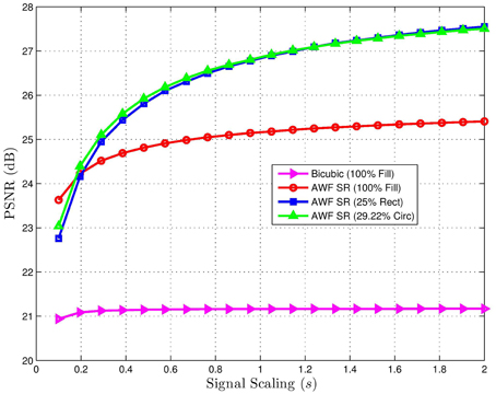
Figure 23. PSNR for K = 16 multiframe AWF SR for the 8 bit motocross image (kodim05.png) with f = 82.65 vs. signal scaling parameter s. Note that s governs the effective noise variance as shown in Equation (8). The system parameters are the Q = 0.50 row in Table 1. For all but the lowest signal levels, the reduced fill factor detectors produce the highest PSNR results after SR processing. A similar trend is seen with all of the images tested.

FIGURE 24

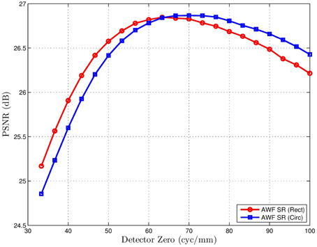
Figure 24. PSNR for K = 16 multiframe AWF SR for the 8 bit motocross image (kodim05.png) vs. the detector zero frequency. The system parameters are the Q = 0.50 row in Table 1, except a and b are changed to control the detector zero location here. The detector zero frequency ranges from 1/p to 1.5/(pQ). Note that the peaks occur very close to the optical cutoff frequency 1/(pQ) = 66.67 cyc/mm.

To see the effect of signal level (integration time) and detector width for square detectors jointly, a PSNR surface plot is shown in Figure 25. This shows the PSNR for AWF SR for the motocross image. Here it can be seen that lower signal levels favor larger detectors. As the scaling s (signal level) increases, small detectors are favored. Interestingly, even for relatively small signal levels, detectors with fill factor less than 100% are still favored. To see the impact on the number of frames used in the SR processing with s = 1, we present the results in Figure 26. Using a small number of frames favors the larger active area images. However, for K > 2, the 25% fill factor images yield higher PSNR results with SR processing. With more frames, the SR processing can better exploit the improved MTF of the small fill factor detectors and can also exploit any redundancy for noise reduction.

FIGURE 25

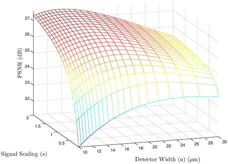
Figure 25. PSNR for K = 16 multiframe AWF SR for the 8 bit motocross image (kodim05.png) vs. square detector width a, and signal scaling parameter s. The system parameters are the Q = 0.50 row in Table 1. Note that for high signal levels (larger s), the optimum a is close to 15 μm (with zero at the optical cutoff frequency 66.67 cyc/mm). However, for very low signals levels (small s), larger active areas are preferred.

FIGURE 26

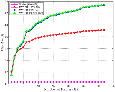
Figure 26. PSNR for multiframe AWF SR for the 8 bit motocross image (kodim05.png) vs. the number of frames K. Shows is the result for a 100% fill factor detector, as well as 25% rectangular and 29.22% circular detectors with zeros at the optical cutoff frequency. Bicubic interpolation of a single frame is also shown for reference. Note that the reduced fill factor detectors benefit more from a larger K as this can help to compensate for the lower SNR.

To show that the benefits of reduced fill factor detectors is not limited to the two images tested thus far, we have included additional quantitative results in Table 2. This tables shows the PSNR for 8 of the Kodak images [21] and the chirp image with 100% fill factor square detectors, 25% fill factor square detectors, and 29.22% fill factor circular detectors. For all of these simulated detectors, we show the PSNR for single frame bicubic interpolation and for multiframe SR processing. The reduced fill factor circular detectors generally provided the highest PSNR values, as might be expected from our analysis. It is interesting to know that even with bicubic interpolation of a single frame (no SR processing), the reduced fill factor detectors are still favored here in most cases. Note that for the results in Table 2, we are using s = 1 and we have a relatively high native SNR.

TABLE 2

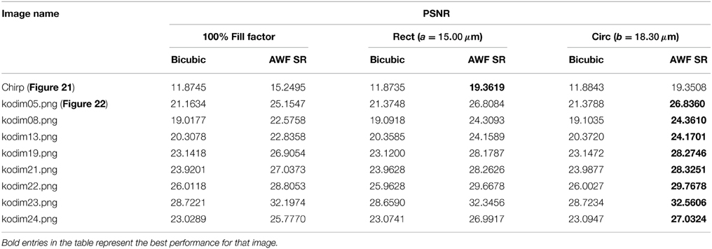
Table 2. PSNR results for AWF SR with K = 16 frames and L = 4 using a variety of 8 bit test images with a simulated MWIR imaging system with Q = 0.50 from Table 1.

5.2. Real MWIR Video

In this section, we present results using an L-3 MWIR camera equipped with F = 4 optics, a native detector pitch of p = 15 μm, and center wavelength of λ = 4.5 μm. The camera is mounted on a tripod and moved with a device to induce small look vector angle variations. This provides translations shifts between frames for SR processing. We employ a high frame rate of 240 fps, to help in minimizing local motion. The robust AWF SR processing detects any local motion and performs single frame restoration in those areas.

In order to compare detector types we have downsampled the imagery by a factor of 2 in each dimension, yielding an effective pitch of p = 30 μm and Q = 0.6. By simply downsampling, we are obtaining square detectors with effective fill factors of approximately 25%. To simulate 100% fill factor square detectors, we average sets of 2 × 2 native pixels prior to downsampling. This averaging lets us obtain pixel values similar to what a single larger active area detector would produce. In this way, we can compare large and small fill factor detectors using an identical scene, optics, read-out electronics, and camera motion. All of the MWIR SR results use K = 16 and L = 3.

The first set of MWIR results is shown in Figure 27. The imagery shows a resolution pattern. The top set contains decreasing 3-bar patterns horizontally and vertically oriented. The scaling is such that moving 6 groups to the right corresponds to a doubling of spatial frequency. The bottom patterns are 4-bar patterns horizontally and vertically oriented. Here, every 4 patterns corresponds to a doubling of spatial frequency. The native p = 15 μm image is shown in Figure 27F, and an ROI of this image is shown in Figure 27E. An L = 3 bicubic interpolation of a single simulated 100% fill factor detector image at p = 30 μm is shown in Figure 27A, and the corresponding 25% fill factor image is shown in Figure 27B. Again, increased aliasing artifacts are evident in Figure 27B. In both of these interpolated images, the last discernible 3-bar pattern in both orientations is 14 patterns from the right. For the 4-bar target, the last discernible pattern appears to be 10 from the right. The AWF SR results for the 100% and 25% fill factor images are shown in Figures 27C,D, respectively. With SR, the last discernible 3-bar pattern is 9 from the right for the 100% fill factor, and 7 from the right for 25% fill factor. The last discernible 4-bar pattern with SR is 7 from the right for the 100% fill factor, and 5 from the right for 25% fill factor. Thus, we see that the SR processing provides an approximately 2× increase in objective resolution, and the reduced fill factor provides an objective boost in resolution compared with 100% fill factor.

FIGURE 27

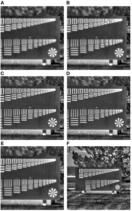
Figure 27. ROI from real MWIR sensor data of resolution chart. (A) L = 3 bicubic interpolation of simulated 100% fill factor detector image at p = 30 μm; (B) bicubic interpolation of simulated 25% fill factor detector image at p = 30 μm; (C) K = 16 and L = 3 AWF SR using 100% fill factor detectors; (D) K = 16 and L = 3 AWF SR using 25% fill factor detectors; (E) native sensor image with p = 15 μm; (F) larger native sensor ROI.

The final set of results is in Figure 28 and Video 1.MOV and shows bleachers at Great American Ball Park in Cincinnati. The native p = 15 μm image is shown in Figure 28F, and an ROI is shown in Figure 28E. An L = 3 bicubic interpolation of a single simulated 100% fill factor detector image at p = 30 μm is shown in Figure 28A, and the corresponding 25% fill factor image is shown in Figure 28B. Again, increased aliasing artifacts are evident in Figure 28B. The AWF SR results for the 100% and 25% fill factor images are shown in Figures 28C,D, respectively. Note that the horizontal bleacher rows are far more discernible in the SR image with 25% detectors, compared with 100%. There is a slight increase in noise, as expected, with the 25% detectors. However, the boost in resolution is very noticeable.

FIGURE 28

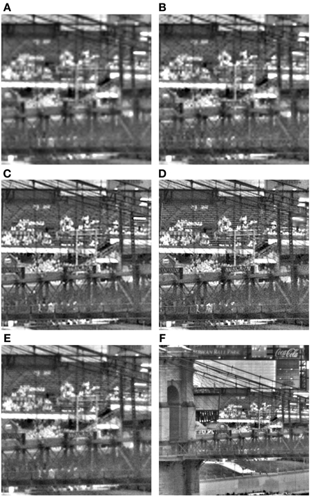
Figure 28. ROI from real MWIR sensor data of bleachers at Great American Ball Park in Cincinnati. (A) L = 3 bicubic interpolation of simulated 100% fill factor detector image at p = 30 μm; (B) bicubic interpolation of simulated 25% fill factor detector image at p = 30 μm; (C) K = 16 and L = 3 AWF SR using 100% fill factor detectors; (D) K = 16 and L = 3 AWF SR using 25% fill factor detectors; (E) native sensor image with p = 15 μm; (F) larger native sensor ROI.

6. Conclusions

In this paper, we have analyzed the impact of detector element active area shape and size on sampling and SR post processing. For 100% fill factor detectors in an imaging system with Q < 1, the detector MTF includes a zero in the band of spatial frequencies that are potentially recoverable using multiframe SR. The basic idea is that reduced fill factor detectors sacrifice signal level, but provide a more favorable overall MTF by pushing the detector MTF zero out toward or beyond the optical cutoff frequency. Post-processing with multi-frame SR can then exploit this expanded spatial frequency content for resolution enhancement. The results in Section 5 show that when a relatively high SNR is available, by virtue of high ambient signal levels and suitable integration times, we can trade some of the high SNR for an improved detector MTF using low fill factor detectors. In a high SNR environment, the optimum detector size is found to be one where the first detector MTF zero is close to the optical cutoff frequency. Thus, our recommendation is that the design of detector active areas be guided by the Q-value for the sensor, if SR is to be used. In particular, for rectangular detectors on imaging systems with Q < 1, we recommend active area dimensions of approximately a₁ = p₁Q and a₂ = p₂Q to put the first detector zero at the optical cutoff frequency. Circular detectors appear to have a slight advantage over rectangular detectors. For circular active area detectors, the first detector MTF zero is located at optical cutoff frequency for b₁ = 1.22p₁Q and b₂ = 1.22p₂Q. In this way, the active area of circular detectors is 1.22²π/4× larger than that of corresponding square detectors. For an imaging system with Q ≥ 1, the first 100% fill factor detector MTF zero is not within the SR folding frequency. Thus, for such systems, there may be no compelling reason to employ reduced fill factor detectors. When reduced active area detectors are used, the extra real estate on the FPA can be used for division of FPA sensing, used as a guard band to minimize diffusion (pixel cross-talk), and/or to allow for opaque electronics. A final note of caution is that with reduced active area detectors we see an increase in aliasing in the observed raw frames. This is due to a decreased low pass filtering effect from detector integration. This can increase the difficulty of discriminating true local scene motion from aliasing artifacts for robust SR [11]. As always, a suitable balance is needed based on the priorities of the sensor application.

Author Contributions

The MTF analysis, algorithm coding, and processing has been done by primarily by RH. DD and MG contributed significantly to the theoretical basis for the paper. AD was instrumental in all data collections and data preparation, and contributed to the various image processing implementations. All authors played a role in analyzing results and preparing the manuscript.

Conflict of Interest Statement

The authors declare that the research was conducted in the absence of any commercial or financial relationships that could be construed as a potential conflict of interest.

Acknowledgments

The authors would like to thank Dr. Ravindra Athale of the Office of Naval Research for the use of the MWIR sensor data. Cleared by Office of Naval Research for public release under Case No. 43-694-14 on 17 December 2014.

Supplementary Material

The Supplementary Material for this article can be found online at: https://www.frontiersin.org/article/10.3389/fphy.2015.00031/abstract

A video showing the MTFs in Figures 11, 13 with variable fill factor ranging from 100% to 0% is provided in Video 2.MOV. This video shows how the zero of the detector MTF moves to higher spatial frequency as the fill factor is reduced. Thus, the overall MTF is more favorable. A similar video showing the MTF from Figure 15 with scaling relative to 100% fill factor detectors is provided in Video 3.MOV. Here the gain relative to the 100% fill factor detector is incorporated. Thus, as the detector zero moves to higher spatial frequency, the overall system gain goes down. However, for a system with a high SNR, this trade can be beneficial.

A video showing the MWIR results for Great American Ball Park from Figure 28 is provided in the file Video 1.MOV. The upper left hand corner is 100% fill factor single frame bicubic interpolation and the upper right hand corner is the robust AWF SR output using 100% fill factor detectors (when the red box appears). The lower left hand corner is 25% fill factor single frame bicubic interpolation and the lower right hand corner is the robust AWF SR output using 25% fill factor detectors (when the red box appears). The increase in resolution is apparent with the 25% fill factor detectors, but also an increased in noise. Note also that the robust AWF SR processing is allowing for the local motion of the pedestrians [11].

References

1. Boreman GD. Basic Electro-Optics for Electrical Engineering. Vol. 31. SPIE Press, Bellingham, WA. (1998). Bellingham, Washington, USA

Google Scholar

2. Reddy RK, Walsh MJ, Schulmerich MV, Carney PS, Bhargava R. High-definition infrared spectroscopic imaging. Appl Spectrosc. (2013) 67:93–105. doi: 10.1366/11-06568

PubMed Abstract | CrossRef Full Text | Google Scholar

3. Park SC, Park MK, Kang MG. Super-resolution image reconstruction: a technical overview. IEEE Signal Process Mag. (2003) 20:21–36. doi: 10.1109/MSP.2003.1203207

PubMed Abstract | CrossRef Full Text | Google Scholar

4. Hardie RC, Schultz RR, Barner KE. Super-resolution enhancement of digital video. EURASIP J Adv Signal Process. (2007) 2007:19. doi: 10.1155/2007/20984

PubMed Abstract | CrossRef Full Text | Google Scholar

5. Katsaggelos AK, Molina R, (eds.). Super resolution (special issue). Comput J. (2009) 52:395–6. doi: 10.1093/comjnl/bxp029

CrossRef Full Text

6. Milanfar P, (ed.). Super-Resolution Imaging. CRC Press (2010). Available online at: http://www.crcpress.com/product/isbn/9781439819302

7. Goodman J. Introduction to Fourier Optics, 3rd Edn. Roberts and Company Publishers (2004). Available online at: http://www.amazon.com/exec/obidos/redirect?tag=citeulike07-20&path=ASIN/0974707724

8. Hardie RC. A fast super-resolution algorithm using an adaptive Wiener filter. IEEE Trans Image Process. (2007) 16:2953–64. doi: 10.1109/TIP.2007.909416

PubMed Abstract | CrossRef Full Text | Google Scholar

9. Driggers RG, Vollmerhausen R, Reynolds JP, Fanning J, Holst GC. Infrared detector size: how low should you go? Opt Eng. (2012) 51:063202. doi: 10.1117/1.OE.51.6.063202

CrossRef Full Text | Google Scholar

10. Hardie RC, Barnard KJ, Ordonez R. Fast super-resolution with affine motion using an adaptive Wiener filter and its application to airborne imaging. Opt Express (2011) 19:26208–31. doi: 10.1364/OE.19.026208

PubMed Abstract | CrossRef Full Text | Google Scholar

11. Hardie RC, Barnard KJ. Fast super-resolution using an adaptive Wiener filter with robustness to local motion. Opt Express (2012) 20:21053–73. doi: 10.1364/OE.20.021053

PubMed Abstract | CrossRef Full Text | Google Scholar

12. Davis M, Greiner ME, Sanders JG, Wimmers JT. Resolution Issues in InSb Focal Plane Array System Design. (1998). Available online at: http://dx.doi.org/10.1117/12.317596

13. Seib DH. Carrier diffusion degradation of modulation transfer function in charge coupled imagers. Electron Devices IEEE Tran. (1974) 21:210–7. doi: 10.1109/T-ED.1974.17898

CrossRef Full Text | Google Scholar

14. Tyo JS, Goldstein DL, Chenault DB, Shaw JA. Review of passive imaging polarimetry for remote sensing applications. Appl Opt. (2006) 45:5453–69. doi: 10.1364/AO.45.005453

PubMed Abstract | CrossRef Full Text | Google Scholar

15. Karch BK, Hardie RC. Adaptive Wiener filter super-resolution of color filter array images. Opt Express (2013) 21:18820–41. doi: 10.1364/OE.21.018820

PubMed Abstract | CrossRef Full Text | Google Scholar

16. Hardie RC, LeMaster DA, Ratliff BM. Super-resolution for imagery from integrated microgrid polarimeters. Opt Express (2011) 19:12937–60. doi: 10.1364/OE.19.012937

PubMed Abstract | CrossRef Full Text | Google Scholar

17. Makitalo M, Foi A. Poisson-Gaussian denoising using the exact unbiased inverse of the generalized anscombe transformation. In: Acoustics, Speech and Signal Processing (ICASSP), 2012 IEEE International Conference on. IEEE, Kyoto (2012). p. 1081–4.

18. Makitalo M, Foi A. Optimal inversion of the generalized anscombe transformation for Poisson-Gaussian noise. IEEE Trans Image Process (2013). 22:91–103. doi: 10.1109/TIP.2012.2202675

PubMed Abstract | CrossRef Full Text | Google Scholar

19. Fiete RD. Image quality and λ FN/ p for remote sensing systems. Opt Eng. (1999) 38:1229–40.

Google Scholar

20. Hardie RC. Super-resolution using adaptive Wiener filters. In: Milanfar P, editor. Super-Resolution Imaging (Series: Digital Imaging and Computer Vision). Taylor&Francis/CRC Press (2010). p. 35–61. Available online at: http://www.crcpress.com/product/isbn/9781439819302

21. Franzen R. Kodak Lossless True Color Image Suite. (2010). Available online at: http://r0k.us/graphics/kodak/