Optimal Paths Between Parameter Estimates in Non-linear ODE Systems Using the Nudged Elastic Band Method

1. Introduction

Ordinary differential equation (ODE) models are widely used for modeling in many scientific areas like physics, engineering econometrics, as well as, in the biomedical life sciences [1]. These types of models are utilized for understanding neural systems, social systems, the WWW, food webs, electrical power grids, tumor cell kinetics, or the dynamics of infectious diseases. Here, we focus on the context of systems biology, where intracellular systems like protein interaction networks, e.g., in signal transduction pathways or gene regulatory networks are described, as well as, intercellular processes of cell populations are investigated [2–6].

The topology of the model and its parameters comprise the interaction of the model components and allow for a quantitative description of the dynamic behavior of the system. Typically, model parameters, i.e., the reaction rate constants of biochemical interactions are not known in all biological conditions and prior knowledge is rarely available, so that the models need to be calibrated by tuning the parameters in order to adequately describe the observations. Experimental data is available from quantitative experimental biology, but typically only a limited number of data points or time courses can be recorded only from parts of the system, and observables are often only accessible through indirect measurement techniques by using antibodies for signal detection. However, observations can be linked to their corresponding biological counterpart in the ODE model and parameters of the model can be estimated and further used for model predictions of e.g., experimentally unaccessible components. Furthermore, the measurement noise has to be quantified and incorporated to the model, in order to assess the uncertainty of the parameters and predictions [7, 8].

The mathematical problem of parameter estimation, i.e., fitting the model to the data, is frequently formulated as finding an optimal parameter set minimizing an objective function, which quantifies the deviation of the model trajectories from the recorded data. To profit from useful statistical properties like consistency and efficiency, this is typically formulated as a maximum likelihood estimation (MLE) [9].

Commonly, models in systems biology are sparse, only partially observed and the ODE systems have solutions which are non-linear with respect to the parameters. Typical models in this field have tens to hundreds of estimated parameters, while the ratio of number of data points to estimated parameters in applications shows a broad spectrum from values slightly larger than one up to ~370 data points per estimated parameter [10]. As the amount of data is often limited and depending on the quality of data, such models yield complex landscapes of the objective function in the high-dimensional parameter search space with a high degree of non-convexity, i.e., inducing the existence of several local optima [10]. Furthermore, non-identifiabilities in the model, i.e., redundancies in the parameterization or the lack of informative data for the determination of some parameters can cause entirely flat manifolds or long skewed and bended valleys in the high-dimensional landscapes, further increasing the complexity of the likelihood landscapes in which optimal parameter values need to be found [8, 11, 12].

High-performance numerical algorithms are available to efficiently tackle the computational complexity of the optimization problem, with prominent examples being e.g., local and global derivative-based deterministic methods, as well as, stochastic particle swarm, simulated annealing or evolutionary approaches [12–16]. The quality of the optimization outcome highly depends on the appropriate choice of the algorithm, as well as, on several user-supplied and pre-defined configurations. Typically, numerical optimizers require configuration parameters as e.g., the maximal number of iterations for termination or tolerances, acting as thresholds either for the step sizes, the evaluated function value or other optimality measures to indicate convergence. If for example the optimizer chooses the size of the next step lower than the defined step tolerance, the algorithm stops, and convergence of the fit is assumed.

These configuration parameters have to be chosen carefully since too strict tolerances do not necessarily yield more accurate results. This may lead to cases where the optimizer continues with too many futile steps, whereas in the opposite situation of not strict enough tolerances, an optimizer is stopped too early and cannot reach the optimum. Adjusting the optimizer tolerances is usually a trade-off between computational resources and requested accuracy for the specific application. Unfortunately, for this task only “rule-of-thumb” methods exist and it is up to the user how to properly choose these configuration parameters for a beneficial outcome in applications. Because of the strong dependence of the proper choices of the algorithms and configurations on the model size and quality of data, optimization is still considered as a major bottleneck in the field of mathematical models for life sciences [10, 14, 17, 18].

In this work, we focus on a so-called multistart optimization strategy, i.e., we utilize a local deterministic optimizer which starts from multiple randomly sampled initial guesses. This combination of a local optimization method with a multistart extension which covers the global search requirements has been shown to perform best in similar applications and is commonly used in the field of ODE models in the context of systems biology [3, 16]. As a local deterministic optimizer cannot escape from a suboptimal basin of attraction, the rational for more complex, i.e., non-convex landscapes is to restart optimization from multiple regions in the parameter space in order to preferably cover all basins of attraction.

The results from the multistart optimization procedure can be used to check the performance of the optimization approach. For an adequate choice of tolerances, a certain fraction of fits converge to the same optimum. However, it is often observed that distinct local optima exist, from which the deterministic optimizer once entered cannot escape toward the global optimum [10].

However, when checking the performance of such a multistart optimization procedure, often non-unique parameter estimates are observed, indicating either a suboptimal optimization approach or a large number of local optima. Because typically, only the objective function's value and the estimated parameter values are recorded, further information for assessing the structure of such a complex and high-dimensional landscape is missing, while additional evaluations are computationally expensive. Since the paths between the multistart optimization end points in the objective function landscape are typically unknown and no information about the connectivity of parameter estimates are available, quality control of the multistart optimization result is difficult. From the fits, it cannot be properly distinguished if two parameter estimates are representatives of the same or of distinct and separated optima, as appropriate methods for finding optimal paths in these complex landscapes and for checking the connectivity of parameter estimates are not available.

A reason for such a suboptimal multistart optimization outcome might be either a too small sample size of the initial guesses compared to the actual number of local optima. Or, on the other hand this could be the result of an inadequate optimizer setup, where more fits should have been converged to the same likelihood value, but instead stopped before reaching the optimum and thus causing a rather continuous distribution of likelihood values.

To overcome the issue of limited interpretability of the multistart optimization results due to the lack of methods to evaluate connectivity of parameter estimates in complex landscapes, we adapt optimal path finding methods in high dimensions from the field of theoretical chemistry, where smooth transition states are computed in a similar setting. For this, we present the analysis of optimal paths between the parameter estimates by utilizing the nudged elastic band (NEB) method in the context of ODE models for systems biology.

Using these methods, a non-trivial path between two points in the high dimensional parameter space can be found and evaluated with controllable and adjustable step size. From inspection of the path's profile, conclusions about the connectivity of the parameter estimates can be drawn. If for example, an optimal path is found which indicates a connection between the two parameter estimates by a smooth transition without exceeding a certain statistical threshold in terms of the objective function value, then all evaluated parameter vectors along this path are equally well in accordance with the analyzed data. If further convexity of the path's profile is fulfilled, any parameter vector from this set can be chosen as a representative of the respective optimum. We further illustrate, how this approach can be used to merge fits from a multistart optimization result to groups of representatives of distinct and separated optima.

2. Methods

2.1. Mechanistic Modeling and Parameter Estimation

A dynamical model is defined by a set of coupled ordinary differential equations (ODE):

$\begin{array}{ll}\dot{x}=f(x(t),u(t),{\theta }_k)& (1)\end{array}$

describing the temporal evolution of states x(t), which in the context of biochemical reaction networks are concentrations of cellular components, e.g., proteins. Their interactions within the mechanistic model are characterized by rate equations f comprising external inputs u(t), as well as, dynamical model parameters θ_k, e.g., reaction rate constants. Initial values x₀: = x(t = 0) of the states can also be treated as unknown parameters θ_init of the model. Solutions of the system in the form of Equation (1) are non-linear with respect to the parameters and need to be integrated numerically.

Observations of the biological system often depend on e.g., the availability of specific antibodies, so that usually only parts of the system can be experimentally accessed and time courses with limited number of time points and few repetitions are feasible. Due to the properties of experimentation techniques in molecular and cell biology, the generated data:

$\begin{array}{ll}{y}^{data}=g(x(t),{\theta }_{obs})+ϵ& (2)\end{array}$

has to be linked via observation functions g to the model states x(t), comprising observation parameters θ_obs, such as e.g., scalings and offsets. Typically Gaussian noise $ϵ~{N}(0,{\sigma }^2)$ with unknown standard deviation σ is assumed, while the presented methodology would also allow for other distributions, as well as, for more complex error models σ(θ_σ, x(t)) with unknown error model parameters θ_σ.

The dynamic model in Equation (1) and the observation functions in Equation (2) are fully described by the parameter set θ: = {θ_k, θ_init, θ_obs, θ_σ} which needs to be calibrated in order to adequately describe the data. For this, the discrepancy between experimental data $y_i^{data}$ and model trajectories y_i(θ) = g(x(t_i), θ) needs to be minimized by finding the optimal parameter set, i.e., the maximum likelihood estimate [9]:

$\begin{array}{l}{\theta }_{MLE}^{\ast }=\underset{\theta }{\text{arg max}}\ell (y|\theta )=\underset{\theta }{\mathrm{arg }\mathrm{ min}}\left(-2\log \ell (y|\theta )\right)\\ =\underset{\theta }{\mathrm{arg }\mathrm{ min}}{\chi }^2(\theta )& (3)\end{array}$

with likelihood function ℓ. In the case of Gaussian noise ϵ this coincides with weighted least-squares estimation [19, 20], i.e., minimization of:

$\begin{array}{ll}{\chi }^2(\theta )={\displaystyle \sum _i}\frac{{\left(y_i^{data}-y_i(\theta )\right)}^2}{{\sigma }_i^2}.& (4)\end{array}$

As a result from Equation (3), we refer in the following to minimization of the negative log-likelihood −2logℓ(y|θ) =: L(θ) as to finding a minimum in the likelihood landscape throughout the manuscript for simplicity and convenience. To ensure positivity in the parameters, which is reasonable in the context of biological systems and in order to improve numerical stability, all parameters are log₁₀ transformed as suggested e.g., in Hass et al. [10] and Kreutz [21].

Likewise to the solutions of the ODEs, the likelihood functions are non-linear with respect to the parameters, which makes parameter estimation, i.e., optimization a non-trivial task, demanding for efficient numerical algorithms. Moreover, powerful optimization algorithms require efficient and reliable gradient information of the likelihood. Therefore, the inner derivatives ∂x/∂θ are needed and can be calculated using the sensitivity equations:

$\begin{array}{ll}\frac{\text{d}}{\text{d}t}\frac{\text{d}x}{\text{d}\theta }=\frac{\partial f}{\partial x}\frac{\partial x}{\partial \theta }+\frac{\partial f}{\partial \theta }.& (5)\end{array}$

While the partial derivatives ∂f/∂x and ∂f/∂θ can be derived analytically, the sensitivities are obtained by solving an additional ODE system with dimension dim(x) × dim(θ) which is attached to the original ODE system from Equation (1) and solved simultaneously [22]. Using the sensitivity equations is superior to the finite differences approximation approach as it is faster and numerically more stable [16].

The Data2Dynamics modeling environment [23, 24] utilizes the CVODES-package of the SUNDAILS Suite [25] for numerical ODE integration and the MATLAB function lsqnonlin [26] as local deterministic optimizer. This approach is combined with a multistart optimization method, i.e., optimization is repeated for multiple randomly drawn initial guesses. For each initial guess, the optimizer is used to fit the model to the data, i.e., an optimal value of the likelihood is calculated and the optimization end point is recorded. The performance of such a multistart optimization procedure is typically assessed by so-called waterfall plots, as described in section 3.1. However, in the case of a suboptimal outcome, it is unclear how to proceed as no conclusion about the connectivity of the parameter estimates can be drawn from the waterfall plot. As demanded in Kreutz [17], we present a methodology which enables to discriminate between the reasons for suboptimal multistart optimization result by assessing the connectivity of parameter estimates.

2.2. Path Finding in High-Dimensional Landscapes

In order to be able to further extend the usage of the waterfall plot by checking the connectivity of parameter estimates, efficient methods are necessary to identify also non-trivial connections between points in the parameter space. Identification of minimal energy paths and free energy barriers in high-dimensional landscapes is a well-known and actively discussed task, especially in the field of computational chemistry and physics of molecular dynamics for finding smooth transitions states of chemical components [27–30]. There, in analogy to the described ODE models, evaluation of the objective function is rather expensive in terms of computational resources, such that sampling the high-dimensional parameter space is not practical and path finding remains a non-trivial task.

Several algorithms and methods have been applied and extended, like the so-called nudged elastic band (NEB) method which is currently one of the state-of-the-art approaches for optimal path finding in computational chemistry [31, 32]. Therefore, we adapt the NEB method for likelihood landscapes of non-linear ODE models in the context of systems biology in the following and utilize it to analyze the connectivity of parameter estimates from multistart optimization sequences.

2.3. Nudged Elastic Band Method

Spring methods for path finding, are characterized by an elastic band or a chain-of-states which is applied to a high-dimensional landscape and converges to an optimal path between its two fixed end points, as depicted in Figure 1A. The presented concept uses the analogy of a chain of nodes which are pairwise connected by springs.

FIGURE 1

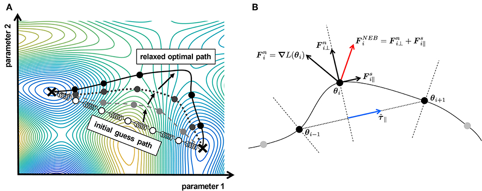
Figure 1. Spring methods for path finding. (A) An elastic band with initial nodes (white dots) connected by springs is relaxed in an illustrative likelihood landscape. The dashed light gray band illustrates an intermediate step during relaxation according to the forces in Equation (8). The dark gray band with the dotted line depicts the state of equilibrating forces for a large spring constant k, which does not completely converge to the minimal, i.e., optimal path. The black solid line and circles represent the final state of a band with adequately small spring constant k and coincides with the optimal path. (B) Nudged Elastic Band (NEB) with forces according to Equations (9) and (10). The blue arrow represents the tangent along the path of the i-th node, characterizing the hyperplane (dashed line) on which the node is constrained.

Two forces are assumed to act on each node: A natural force, which moves the individual node toward lower regions in the landscape, following a steepest descent based on the negative gradient of the landscape at the individual node. The second force represents the attracting force of a hypothetical spring connecting two nodes. It hinders the nodes from freely moving through the landscape, but instead seeks to equate the distance between the adjacent nodes. A relaxed band, i.e., the position of the nodes in which all forces are in the equilibrium represents the final state and defines the optimal path.

The nodes θ_i are connected by springs to their neighbors θ_i−1 and θ_i+1 and the so-called spring forces:

$\begin{array}{ll}{F}_i^s=k({\theta }_{i+1}-{\theta }_i)-k({\theta }_i-{\theta }_{i-1})& (6)\end{array}$

with spring constant k ensure an adequate distribution of the nodes along the path. By this, the nodes are prevented from moving uncontrollable in the force field of the natural force:

$\begin{array}{ll}{F}_i^n=-\nabla L({\theta }_i),& (7)\end{array}$

i.e., the force at the respective nodes caused by the local gradient of the likelihood function L(θ_i). In this basic formulation, the band is initialized on an initial path Θ = {θ₀, …, θ_i, …, θ_end}, which is chosen to be the direct connection between the fixed end points θ₀ an θ_end with N evenly distributed free nodes in-between.

In the so-called relaxation phase, the band converges to the optimal path by moving the free nodes and thus equilibrating the forces:

$\begin{array}{ll}{F}_i=F_i^n+F_i^s& (8)\end{array}$

on all nodes of the band (c.f. bands in Figure 1A). Depending on the actual geometry of the likelihood landscape, the number of free nodes N and the spring constant k need to be adjusted in order to find a suitable optimal path.

It has been shown that this basic formulation has some disadvantages, i.e., corner-cutting for large k or down-sliding for weaker spring forces, leading to either a poor resolution in the vertex of a valley (c.f. band with solid black line in Figure 1A) or a slightly less optimal path compared to the true optimal path (c.f. gray dotted band in Figure 1A), respectively [31].

To overcome these issues, the nudged elastic band (NEB) method has been proposed [31] and is considered as one of the standard methods [33] of molecular dynamics in theoretical chemistry. The idea of a nudged band is to disentangle the forces:

$\begin{array}{ll}{F}_i^{NEB}:=F_{i\perp }^n+F_{i\left|\right|}^s& (9)\end{array}$

on the band nodes, by projecting the spring contributions on the normalized tangent ${\widehat{\tau }}_i$ of the path at θ_i, as illustrated in Figure 1B. For the natural force:

$\begin{array}{ll}{F}_{i\perp }^n=-\nabla L({\theta }_i)+\left(\nabla L({\mathit{\theta }}_i)·{\widehat{\tau }}_i\right){\widehat{\tau }}_i,& (10)\end{array}$

only the force perpendicular to the path tangent is considered, such that the displacement of the free nodes by the natural force is constrained on the local perpendicular hyperplanes. This key feature of the NEB method circumvents that a node moves constantly in direction of one of its two neighbors θ_i−1 and θ_i+1 driven by the components of the local natural force along the path. Without disentangling the forces, the nodes of the band would predominantly move toward the fixed end points θ₀ and θ_end, instead of exploring the space in-between. The spring force $F_{i\left|\right|}^s=(F_i^s·{\widehat{\tau }}_i){\widehat{\tau }}_i$ on the other hand, is restricted to the tangential component along the path, seeking only an equal spacing between the nodes, i.e., the hyperplanes without inferring the optimization guided by the natural force on the hyperplanes.

The optimal path is characterized by the set of parameters ${\Theta }^{*}=\left\{{\theta }_0,\dots ,{\theta }_i,\dots ,{\theta }_{end}\right\}$ equilibrating all forces, i.e., minimizing the functional:

$\begin{array}{ll}{S}^{NEB}\left({\theta }_0,\mathrm{...},{\theta }_i,\mathrm{...},{\theta }_{end}\right)=\underset{\text{natural forces}}{\underbrace{{\displaystyle \sum _{i=1}^{N}L}\left({\theta }_i\right)}}+\underset{\text{spring forces}}{\underbrace{{\displaystyle \sum _{i=0}^N\frac{k}{2}}{\left({\theta }_i^{{\tau }_i}-{\theta }_{i+1}\right)}^2}}& (11)\end{array}$

with restriction on the aforementioned hyperplanes at ${\theta }_i^{{\tau }_i}$ with orientation defined by the constraint ${\theta }_i·{\widehat{\tau }}_i=0$. The minimized functional can be interpreted as total energy of the band, consisting of the potential energy contributions at the nodes resulting in the natural forces and the spring potential from the springs between the nodes resulting in the spring forces. The discussed geometrical constraints i.e., the restriction on the hyperplanes reflects the nudging feature of the band, i.e., the disentanglement of natural and spring forces in order to ensure an equal spacing of the nodes along the optimal path.

For implementation of the NEB concept within our modeling framework, we realize N copies of the considered ODE model and constrain optimization of the parameters of each copy of the model to the respective hyperplane perpendicular to the path tangent, by manipulating the individual gradients according to Equation (10). A local deterministic optimizer is used to minimize the path functional ${{S}}^{NEB}$, which comprises N × dim(θ_i) free parameters and requires parallel evaluation of N-times the model equations. The implementation and sample scripts are available within the D2D framework for modeling of ODE models [24].

3. Results

In the following section, we discuss how interpretability of the results of a multistart optimization can be increased. It is presented, under which circumstances two parameter estimates can be grouped together and assumed to be representatives of the same optimum. As a proof-of-concept, we apply the NEB path finding and multistart optimization merging approach to a well-known signal transduction model from the literature with experimental data and confirm the capacity of the proposed methodology to uncover the local optima structure by merging fits from a suboptimal multistart optimization result.

3.1. Inspection of Waterfall Plots

The results of a multistart optimization sequence are typically illustrated for visual inspection in the so-called waterfall plot [16, 34], where the fits are ordered by their optimization outcome, i.e., by the likelihood value of the individual optimization end points. The waterfall plot serves to identify groups of fits with the same likelihood value after optimization, assuming that they belong to the same local optimum. Thus, from the form of the waterfall plot, conclusions about the optimization performance, as well as, about the local optima structure of the likelihood can be drawn.

We use two illustrative likelihood landscapes depicted in Figure 2 to discuss the concept of the waterfall plot and its interpretability. The likelihood landscape with two parameter dimensions in Figure 2A reveals four separated optima. In analogy to a multistart optimization procedure in applications, initial values are drawn randomly from the whole parameter space. In the high-performance setting of the optimizer, the algorithm starts from the individual initial guesses and fully converges to one of the optima. In the suboptimal numerical setting, the optimization algorithm is insufficient in most cases, i.e., it is unable to converge to one of the optima, as it erroneously stops too early. The performance of the two optimizer configurations can be objectively assessed in the waterfall plot (c.f. Figure 2B). A stair-like plot of four distinct steps, i.e., plateaus with the same likelihood value appears in the waterfall plot, indicating four groups of fits in the high-performance setting. However, the likelihood values of the two intermediate steps are relatively close and not easy to discriminate by visual inspection, so that one tends to erroneously bunch the fits #8–#20 (highlighted in red) of the high-performance setting together in one group.

FIGURE 2

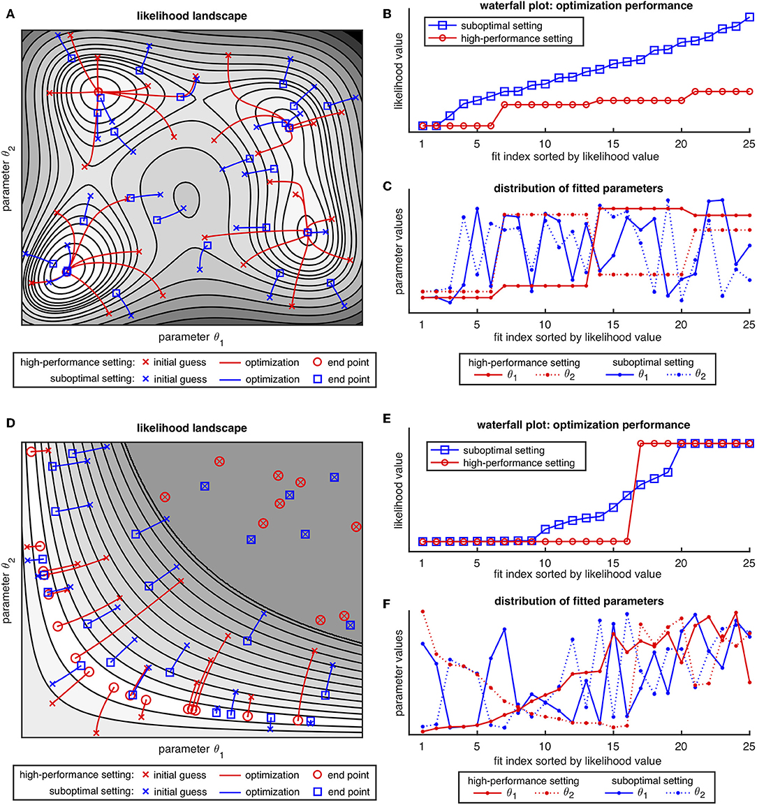
Figure 2. Illustrative likelihood landscapes in (A,D) and resulting waterfall plots in (B,E) with their respective parameter distributions plots in (C,F). A high-performance setting is plotted in red, whereas a suboptimal optimization setup is realized by restricting the maximal number of iterations and depicted in blue.

To circumvent these incorrect interpretations of the waterfall plot, it is recommended to also check the parameter distribution of the fits as depicted in Figure 2C. By this, both, likelihood distances of the fits and the parameter structure can be assessed [35]. In cases, where the optimizer did not fully converge, a certain correlation in the deviation in terms of objective function value and distance in the parameter space between two similar fits is expected. From the plot, it can be concluded, that the discussed fits clearly split up into two separated groups with opposing parameter values, indicating two distinct and distant optima in the parameter space.

In contrast, for the suboptimal numerical case, only the two fits with the lowest likelihood value form a step and yield the same parameters. All other fits plotted in blue form a suboptimal waterfall plot with a slope of gradually increasing likelihood values without any distinct stair-like structure. This outcome is supported by the random-like distribution of the parameter values (blue dots) in the panel below. Inspection of panel A reveals that some fits in fact converge to three of the four optima, however in applications with a similar suboptimal result, the true number of local optima is not indicated in the waterfall plot and, more importantly, it cannot be concluded, that the global optimum is found, as a larger sample size of the initial guesses might reveal additional optima with lower likelihood value.

A second typical likelihood landscape is illustrated in Figure 2D. It does not possess a unique optimum, but rather reveals a bended valley-like structure at the lowest likelihood level. Furthermore, it contains a flat manifold in the upper right corner, where the gradient for all initial values is zero and thus all fits immediately stop without moving toward an optimum. Both structures are typical cases of either structural or practical non-identifiabilities in the likelihood [8, 11], which are a consequence of over-parameterization of the model or appear when the information provided by the available data is not sufficient to restrict parameters to finite confidence intervals, respectively.

In the well-performing setting of the optimization setup, all fits outside the flat region converge to a point at the lowest level of the likelihood valley. This yields a waterfall plot like in Figure 2E with two distinct plateaus. Again, one would erroneously tend to conclude that two distinct and unique optima are found. However, inspection of the parameter distribution plot in Figure 2F shows 16 different parameter estimates with the same minimal likelihood value. While a functional relation, i.e., an inverse correlation of the parameter values on the lowest step can be easily detected and linked to a non-identifiability of e.g., two coupled model parameters, the parameter estimates from the highest step all have the same likelihood value, but exhibit a random-like distribution in their parameter values. Similar conclusions can be drawn from the blue fits of the suboptimal setting in Figures 2D–F but in addition, the waterfall plot shows a gradual transition between the two levels, comparable to a “slippery stair.” Likewise to the first example, neither the structure of the waterfall plot, nor the parameter distribution plot can give evidence, if fits #10–#19 (highlighted in blue) are members of the global optimum or if there are local optima in-between.

It should be noted that for applications, explicitly assessing the likelihood landscape like in Figures 2A,D is not feasible and thus, all conclusions need to be drawn from the respective waterfall and parameter distribution plot alone. We surmise that a combination of both presented likelihood scenarios might be the dominant setting in applications, so that there is a particular need for additional tools analyzing the grouping of fits by checking the connectivity between two points in the parameter space.

3.2. Connecting Paths Between Parameter Estimates

To further extend the interpretability of a multistart optimization result and to merge fits of the same optimum together into one group, connections between the fits, i.e., paths between two estimates in the parameter search space are analyzed. Although parameter distribution plots enable to qualitatively assess the distribution of the fits in the parameter space, different physical units and the diverse classes of parameters (e.g., reaction rate constants, initial concentrations, observation, or error parameters) render Euclidean distances between parameter estimates difficult to interpret.

To assess the connectivity of two fits, evaluation of the structure of the likelihood landscape in-between the two points is necessary. For the path profile, likelihood values along a path between two points in the parameter space can be evaluated and its form can be used to analyze their connectivity. For example, a straight line between the two points represents the naïve, yet sometimes efficient approach of the direct path. In a convex landscape, the likelihood profile of such a path from a not fully converged fit to the optimum would be monotonically decreasing (c.f. blue fits in Figure 2A). However, in applications with a slightly more complex landscape like in the example of Figure 2D, a direct path would fail to connect e.g., two optimization end points within the bended valley-like optimum. Thus, we suggest and employ the NEB method in the following in order to take account also for more complex paths in high dimensional likelihood landscapes.

When an optimization run of a parameter estimation procedure did not fully converge to the respective optimal point in the parameter space, monotone or convex path profiles result as a consequence, as depicted in Figures 3A–C for the optimal path, e.g., from a NEB path search. As illustrated in scenario B, such a path could also reveal a new optimum, i.e., a better representative of the same optimum and might be utilized as an additional fine-grain optimization strategy [36]. In applications, more complex tasks, e.g., a saddle point region connected to an optimum, separated optima like in scenarios C-E or bended valleys like in Figure 2D are the predominant challenges, where the direct path qualitatively differs from the optimal paths.

FIGURE 3

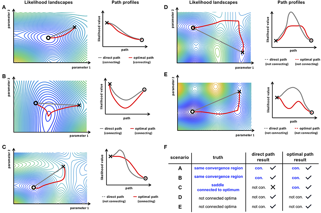
Figure 3. (A–E) Illustrative likelihood landscape scenarios and their respective path profiles revealing connections between two points in the parameter space (× and ◦). The gray line represents the direct path in the likelihood landscape and the respective path profile. The red paths show the outcome of an optimal path finding method, e.g., the NEB method. By this, more complex paths can be found, as for instance in scenario (C), where a connection is denied by the direct path, but an appropriate path finding method reveals the monotonically decreasing connecting path. The table in (F) summarizes conclusions about connectivity of the two points in the respective scenarios. Only the optimal path method is able to adequately draw conclusions about the connectivity of the two points.

In these cases, the direct path shows an increase of the likelihood between the two points. Utilizing a more flexible optimal path finding algorithm, like e.g., the NEB method, a connecting path can be found which in principle would also yield acceptable directions for an optimizer, i.e., the path profile reveals monotonicity along the path as illustrated in Figure 3C. However, for the case of separated optima where no connecting path between the two end points of the path exist, the NEB method would reveal a non-monotonic, concave profile (c.f. Figure 3D).

Another scenario is depicted in Figure 3E, where the optimal path is entirely below the likelihood threshold of the higher end point but does not have a convex profile. In such a case, where a small barrier persist in the path profile, it is concluded that the two points are representatives of separate optima because the barrier would not be surmountable for a local optimizer.

We conclude, that connectivity between two points in the parameter space can be assumed, when a connecting, i.e., convex path between the two points is found. It should be noted at this point, that for finding a connecting path it is sufficient to show connectivity of e.g., a NEB path once. However, using a local optimal path searching method that reveals a non-connecting, i.e., concave path profile, it is not possible to conclude that the corresponding optima are in fact separated, because a convex path might still exist, but the NEB approach might fail to find such a path, e.g., due to a suboptimal initialization. Finding a convex path is sufficient for concluding connectivity but, in contrast, non-convex paths are only necessary, but not sufficient for concluding non-connectivity (c.f. Figure 3F).

3.3. Merging of Multistart Fit Results

Being able to identify fits from the waterfall plot as representatives of the same, i.e., connected local optima by connecting paths as described above, enables to merge the fits resulting from a multistart optimization approach reliably into groups. Starting with the best fit, we generate optimal paths using the NEB method and profiles are checked for connectivity for all subsequent fits. For increasing the efficiency, i.e., lowering the computational cost and combinatorial complexity of the pairwise path finding between two fits, first the initial path, i.e., direct path is evaluated and checked for connectivity.

Connectivity observed by a direct path profile occurs mostly for cases where fits are already close to a local optimum, i.e., are almost fully converged and often also have a small Euclidean distance from each other. In these cases, often the numerical integration accuracy influences the fine-grain surface of the likelihood and more stringent tolerances controlling the numerical accuracy are required.

If the initial path does not reveal a connecting profile, the NEB approach is applied using a large spring constant k. When such a NEB path finding run was not sufficient, i.e., no connecting path was found, the procedure is repeated with a smaller spring constant k in order to allow more flexibility of moving the free nodes in the likelihood landscape. Thus, spring constants are decreased subsequently up to a limit of k = k_min or until a connecting path is found and the fit is identified as representative of the global optimum likewise to the best fit. Both fits are then grouped together in the waterfall plot and excluded from the further pairwise path searches.

Likewise, the procedure is iteratively repeated, starting with the next best fit from the waterfall plot for which a connecting path was not yet found in the previous runs. All remaining fits are subsequently used for pairwise path searches until either a connecting path is found or a fit is declared as the first representative of an isolated local optimum.

3.4. Application to JAK/STAT Signaling Model

In the following we use the JAK/STAT signaling model from Swameye et al. [37] as a proof-of-concept application for the NEB path finding and multistart optimization merging approach. The system consist of four species describing the proteins concentrations of STAT5 and its phosphorylated forms which upon Epo activation at the Epo receptor transduct the activation signal along the intracellular pathway through the cytoplasm into the nucleus and initiate gene transcription. The input function of the external stimulus in form of the measured activated Epo receptor concentration is adapted from Swameye et al. [37] and will not be fitted in the following. The 46 data points were collected from quantitative immunoblotting, i.e., were measured using antibodies and therefore the objective functions include in total four scaling and offset parameters, which are estimated comprehensively with the two respective error parameters and the four rate constants, i.e., dynamic parameters of the described signaling pathway. In total 10 parameters are estimated on the log₁₀ scale and with upper and lower boundaries at ${\theta }_i\in \left[10^{-5},10^3\right]$.

To show the capacity of our approach, we employ the JAK/STAT signaling model as a small and fast to compute benchmark model with two optimizer setups. To be able to investigate the described suboptimal case of waterfall plots in a controlled manner, we use an intentionally suboptimal optimizer setup for generating the multistart optimization result, as well as, for NEB path finding and waterfall plot merging. We mimic a case where the optimizer settings do not match the demands characterized from the model size, quality and amount of the data. For this, we set the step tolerance of the local deterministic optimizer implemented in the MATLAB function lsqnonlin [26] to a very loose value of TolX = 10⁻¹, causing a too early termination of the individual fits. Using a multistart sequence from 50 randomly sampled initial guesses, the best fit in this setting is identical with the published parameter values, i.e., the model trajectories are identical with the published fits from Swameye et al. [37]. To be able to compare the results of the NEB-based waterfall plot merging approach with an appropriate optimizer setup, we perform the analysis with the same initial guesses with the standard setup of the step tolerance, i.e., TolX = 10⁻⁶.

Both resulting waterfall plots are shown in Figure 4. The intentionally suboptimal setting in Figure 4A exhibits a form of the waterfall plot from which an unambiguously clear conclusion about underlying local optima structure cannot be drawn. Likewise, the plot of the distribution of estimated parameters in the panel below does not allow for grouping the fits. The same kind of outcome often appears in applications when using the standard settings of the optimizer with more complex models in terms of number of estimated parameters, number of non-identifiable parameters or amount of informative data points.

FIGURE 4

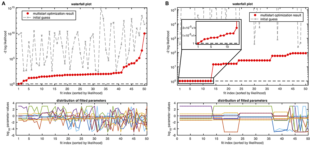
Figure 4. Waterfall plot and distribution of parameters of fits from the same 50 randomly sampled initial guesses in (A) with the suboptimal optimization setup and in (B) with the standard optimization setup using the JAK/STAT signaling model with ten estimated parameters. For illustration, likelihood values are shifted to the baseline of one by subtraction of the likelihood value for the global minimum.

The waterfall plot of the standard setup in Figure 4B shows a favorable structure with 13 fits on the lowest level and ~6 additional steps, indicating convergence of the optimizer in several local optima. From the parameter plot in panel B it can be surmised, that the top 13 fits from the lowest level are close together, as no differences from the best fit parameter vector are visible by eye. However, when zooming in (c.f. inset in Figure 4B), it can be seen that a very small rugged slope is observed, which is in the order of magnitude of numerical resolution. On the higher steps, a similar observation is made but on a larger scale (not shown). Similar to the discussed case in Figure 2, fits #14–#23 cannot be easily distinguished by visual inspection of the likelihood value in the waterfall plot. However, the parameter distribution plot below exhibits the two groups in more detail.

3.5. NEB Method Reveals Optimal Paths in JAK/STAT Signaling Model

To apply the NEB method to the multistart optimization results of the JAK/STAT signaling model, we use 25 free nodes per band between the fixed start and end points, i.e., two parameter estimates or fits from the waterfall plot. Besides the number of free nodes, which corresponds to the resolution of the stepwise linear band, the spring constant k is the most relevant configuration parameter for the NEB path finding. A high value of the spring constant results in a strong attractive force within the band, ensuring equal distances between the nodes, but also less flexibility of sliding away perpendicular to the path, i.e., less flexibility in the orientation and positioning on the hyperplanes for more complex landscapes, as discussed in section 2.3. Thus, is can be assumed that iteratively decreasing the spring constants k gradually increases the level of flexibility in terms of allowing more deviations from the initial path for more complex forms of the path.

Figure 5A shows a set of path profiles for varying spring constants k between fits #1 and #13 of the multistart optimization results from Figure 4A. The initial path, i.e., the direct path between the end points of the band shows a clearly non-connecting path with a distinct increase of the likelihood in-between. The profile coincides with the relaxed NEB path with spring constants of k = 100 and above. When gradually decreasing the spring constants to values of k∈{35, 25, 10}, the likelihood amplitude of the path is substantially lowered and the entire path is below the likelihood value of the highest end point, i.e. fit #13. However, the path profiles for k = 25 and k = 10 still exhibit a non-convex and non-monotone path, from which connectivity of the two parameter estimates cannot be concluded. From this set, only the path profile of the band with spring constant k = 35 yields the appropriate equilibrium of flexibility and cohesion of the band by revealing a monotone path connecting both end points. Interestingly, the same order is observed in Figure 5B, where compared to the NEB paths of k = 25 and k = 10, the blue path of k = 35 is also more distant from the initial path in the parameter space, although the spring constant is larger. When further decreasing the spring constants, even lower paths are found until for very low spring constants like k = 2 and k = 1, the path profile, as well as, the path in the parameter space becomes rugged because of the suboptimal performance of the optimization and due to the too weak attracting spring forces between the nodes for low values of k of the NEB approach.

FIGURE 5

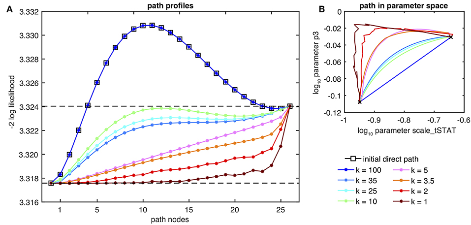
Figure 5. Optimal paths from the NEB method for several spring constants k from fit #1 to #13 of the intentionally suboptimal setup for the JAK/STAT signaling model (c.f. Figure 4A). (A) Shows the path profiles of the NEB approach, as well as, for the initial, i.e., direct path. (B) Depicts the same paths in an illustrative choice parameter dimensions.

3.6. Merging Suboptimal Waterfall Plots

For merging the fits in the following, we apply the optimal path finding strategy as described before for pairs of fits from the multistart optimization results. When the direct path between two parameter estimates shows a non-connecting profile, the NEB method is performed, starting from the largest spring constant of the set k = {200, 100, 50, 20, 10, 5, 2, 1} until a connecting path is found. When such a path is found, it can be assumed that the two parameter estimates are representatives of the same optimum and they are grouped together in the waterfall plot.

First, the waterfall plot from the intentionally suboptimal optimization setup from Figure 4A is used. For a fair comparison, the same suboptimal setting of the optimization algorithm, i.e., a step tolerance of TolX = 10⁻¹ is used for the NEB path finding, as well as, for the merging approach.

The results are presented in Figure 6A. Connecting paths are found for 38 pairs of parameter estimates, whereas 12 fits act as first representatives of the respective optima, implicating that 12 separated optima were found from an originally suboptimal waterfall plot. Before merging, only the first two fits could be identified as representatives of the same optimum and only by visual inspection. All other fits had individual likelihood values, not allowing for grouping based on likelihood or parameter values (c.f. Figure 4A). In total, 22 fits are grouped together on the lowest step, i.e., to the global optimum. These fits are merged from sometimes large distances in the likelihood value, with diverse spring constants k, indicated by the different colors of the circles in the waterfall plot. Interestingly, all nine fits with the highest likelihood value could be merged to the lowest, i.e., the best fit.

FIGURE 6

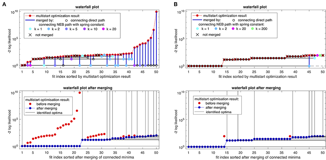
Figure 6. Merged waterfall plots. In (A) with the intentional suboptimal optimization setup and in (B) with the standard optimization setup. The top row shows the waterfall plot before merging the fits based on found connecting paths, indicated by the colored circles on the level of the corresponding first representative of the connected optimum. The colors indicate the first successful connecting path using a spring constant from the set k = {200, 100, 50, 20, 10, 5, 2, 1}. The bottom row shows the resulting merged and reordered waterfall plots. For illustration, likelihood values are shifted to the baseline by subtraction of the likelihood value for the global minimum.

The merging approach was also applied to the waterfall plot from Figure 4B, which is the result of a multistart optimization with the same initial values as in Figure 4A, but with the standard choice of the optimizers' step tolerance, i.e., TolX = 10⁻⁶.

Since the first 13 fits of the waterfall plot had very similar likelihood values with differences only in the order of numerical accuracy (c.f. inset of Figure 4B), the direct path is in most cases sufficient for finding a connecting path, as indicated in Figure 6B by the black circles. Although it is already expected from the relatively flat lower step in the waterfall plot and from the clear parameter distribution plot in Figure 4B, it can now be reliably concluded, that these fits belong to the same optimum. Besides the majority of the fits which can be merged by direct paths in the standard setting of the optimizer, proving connectivity of the fits, i.e., membership of the respective optima, there are four fits (#45, #47–#49) with higher likelihood for which NEB path-based merging with diverse spring constants was necessary. Interestingly, a connecting path from fit #45 to the best fit #1 was found, indicating that even for relatively strict tolerances of the optimizer, the NEB method may provide additional connectivity within the likelihood landscape. In conclusion, the waterfall plot after merging reveals six optima with more than one representatives.

The merged waterfall plot of the suboptimal optimizer settings reveals seven optima with more than one representatives but with a very large first step, i.e., 22 representatives of the global optimum. The reason for this might be that these not fully converged fits stopped in regions of the parameter space where flat manifolds of the likelihood appear and thus, optimal paths to different regions, i.e., optima are achievable. Moreover, for an appropriate optimizer setup it may be possible that the optimizer makes large efficient steps toward other basins of attraction. As a consequence, the merged waterfall plot of the reference case, i.e., with the appropriate choice of optimizer configurations, yields less fits in the global optimum but more fits in the higher steps, i.e., local optima of the waterfall plot.

The computation time for the multistart optimization from 50 initial guesses on a single core of a 3.4 GHz CPU was 16 s for the suboptimal optimizer setting and 59 s for the standard setting. In comparison, computational demands for the whole merging procedure are much higher, as calculations for the suboptimal setting take 1.9 h and 18.1 h for the standard optimizer setting. This long time results from the sequential pairwise path searching approach, where a relatively large number of paths with small spring constants k need to be computed. Partially parallelizing the approach or re-ordering of the NEB path finding, i.e., trying first direct paths on all pairs and then calculate the NEB path for the remaining fits may increase the speed, and might be chosen by the user depending on expected outcome in other applications.

4. Discussion and Conclusion

Parameter estimation in non-linear ODE models with data from quantitative experimental biology is challenging, so that appropriate optimization strategies have to be utilized and properly configured. A powerful instrument is the usage of a multistart optimization strategy in combination with a local deterministic optimizer. However, in applications the outcome of such an approach may still be difficult to be interpreted, when waterfall plots show non-unique parameter estimates and parameter distribution plots exhibit strongly varying parameter values. In such cases, groups of fits cannot be identified reliably from the likelihood values in the waterfall plot or the parameter values alone. Furthermore, Euclidean distances between the parameter estimates cannot be used for merging the fits, since the connectivity in the likelihood landscape between the estimates is unknown.

Evaluating whether two results of a parameter estimation procedure belong to the same local optimum enables to further improve the interpretability of the multistart optimization result. Thus, we present an approach which incorporates optimal path finding concepts from the field of molecular dynamics in theoretical chemistry and enables to compute and analyze likelihood profiles between parameter estimates. Herewith, a reliable grouping of the parameter estimates is ensured and enables the possibility of merging fits in the waterfall plot. As a consequence, it can be more precisely assessed how often the global optimum is found and how many local optima are comprised in the likelihood. In applications, the insights might be used to invest the limited computational resources either into a larger sample size of the initial guesses for the multistart optimization procedure, or in a fine-tuned optimizer setup with stricter tolerances and increasing convergence frequency of the individual fits.

As presented in this work, the basic formulation of the nudged elastic band (NEB) method for path finding yields satisfactory results in the proof-of-concept application of the JAK/STAT signaling model. There, our approach was applied to a small benchmark model with experimental data in an intentionally suboptimal setting of the configuration of the optimization algorithm. By merging the fits with connecting path profiles, we could process the suboptimal waterfall plot to a preferable stair-like form of the waterfall plot.

After all, computational costs for such a complete merging of a multistart optimization result are relatively high. Moreover, the issue of suboptimal waterfall plots arises predominantly in larger scale models, where evaluation of the model equations and thus also parameter estimation is computationally even more demanding. Because of the relatively high computational demands for path finding, the presented approach is rather suitable to examine problematic cases where optimization is difficult and does not yield satisfying results while the reasons for this behavior remain unclear. Furthermore, in cases where local optima cannot be statistically excluded after a multistart optimization run, as they are below a certain threshold in terms of the likelihood value and are thus also in accordance with the data, the presented approach enables to examine the connectivity of single fits. In such cases it could be e.g., of interest, if there is a smooth transition between the respective trajectories of the model for various fits or, if the fits belong to distinct optima in the parameter space and e.g., additional data is required to reveal the true underlying biological mechanism.

However, several extensions have been discussed for the NEB method, such as the introduction of smoothing terms [31, 38], alternative path tangents [39], climbing image approaches for improved saddle point searches [40, 41], as well as, the usage of Gaussian processes [42] and combinations with machine learning approaches [43] in the context of analyzing transition states of chemical systems. We surmise, that analysis of ODE models using the NEB method likewise benefits from adaptions of these approaches, especially for larger models with more parameters to be estimated. For this, applicability and costs needs to be checked carefully in the systems biology related ODE model setting and is open to further research.

Data Availability Statement

The data analyzed for this study and the code to reproduce the results can be found within the MATLAB-based Data2Dynamics modeling environment: https://github.com/Data2Dynamics/d2d/tree/master/arFramework3/Examples/NEB.

Author Contributions

CT and CK conceived the idea. CT designed the study, implemented the method, conducted the simulations and analysis, and carried out drafting. JT and CK supervised the project and contributed to manuscript writing.

Funding

This study was supported by the German Research Foundation (DFG) under Germany's Excellence Strategy (CIBSS–EXC-2189–Project ID 390939984). The article processing charge was funded by the German Research Foundation (DFG) and the University of Freiburg in the funding programme Open Access Publishing.

Conflict of Interest

The authors declare that the research was conducted in the absence of any commercial or financial relationships that could be construed as a potential conflict of interest.

References

1. Xue H, Miao H, Wu H. Sieve estimation of constant and time-varying coefficients in nonlinear ordinary differential equation models by considering both numerical error and measurement error. Ann Stat. (2010) 38:2351–87. doi: 10.1214/09-AOS784

PubMed Abstract | CrossRef Full Text | Google Scholar

2. Busch K, Klapproth K, Barile M, Flossdorf M, Holland-Letz T, Schlenner SM, et al. Fundamental properties of unperturbed haematopoiesis from stem cells in vivo. Nature. (2015) 518:542–6. doi: 10.1038/nature14242

PubMed Abstract | CrossRef Full Text | Google Scholar

3. Steiert B, Raue A, Timmer J, Kreutz C. Experimental design for parameter estimation of gene regulatory networks. PLoS ONE. (2012) 7:e40052. doi: 10.1371/journal.pone.0040052

PubMed Abstract | CrossRef Full Text | Google Scholar

4. Becker V, Schilling M, Bachmann J, Baumann U, Raue A, Maiwald T, et al. Covering a broad dynamic range: information processing at the erythropoietin receptor. Science. (2010) 328:1404–8. doi: 10.1126/science.1184913

PubMed Abstract | CrossRef Full Text | Google Scholar

5. Kholodenko BN. Cell-signalling dynamics in time and space. Nat Rev Mol Cell Bio. (2006) 7:165–76. doi: 10.1038/nrm1838

PubMed Abstract | CrossRef Full Text | Google Scholar

6. Schoeberl B, Eichler-Jonsson C, Gilles ED, Müller G. Computational modeling of the dynamics of the MAP kinase cascade activated by surface and internalized EGF receptors. Nat Biotechnol. (2002) 20:370–5. doi: 10.1038/nbt0402-370

PubMed Abstract | CrossRef Full Text | Google Scholar

7. Kreutz C, Raue A, Timmer J. Likelihood based observability analysis and confidence intervals for predictions of dynamic models. BMC Syst Biol. (2012) 6:120. doi: 10.1186/1752-0509-6-120

PubMed Abstract | CrossRef Full Text | Google Scholar

8. Raue A, Becker V, Klingmüller U, Timmer J. Identifiability and observability analysis for experimental design in nonlinear dynamical models. Chaos. (2010) 20:045105. doi: 10.1063/1.3528102

PubMed Abstract | CrossRef Full Text | Google Scholar

9. Cox DR, Hinkley DV, Barndorff-Nielsen OE. Time Series Models: In Econometrics, Finance and Other Fields. Boca Raton, FL: CRC Press (1996).

Google Scholar

10. Hass H, Loos C, Raimúndez-Álvarez E, Timmer J, Hasenauer J, Kreutz C. Benchmark problems for dynamic modeling of intracellular processes. Bioinformatics. (2019) 35:3073–82. doi: 10.1093/bioinformatics/btz020

PubMed Abstract | CrossRef Full Text | Google Scholar

11. Raue A, Kreutz C, Maiwald T, Bachmann J, Schilling M, Klingmüller U, et al. Structural and practical identifiability analysis of partially observed dynamical models by exploiting the profile likelihood. Bioinformatics. (2009) 25:1923–9. doi: 10.1093/bioinformatics/btp358

PubMed Abstract | CrossRef Full Text | Google Scholar

12. Transtrum MK, Machta BB, Sethna JP. Geometry of nonlinear least squares with applications to sloppy models and optimization. Phys Rev E. (2011) 83:036701. doi: 10.1103/PhysRevE.83.036701

PubMed Abstract | CrossRef Full Text | Google Scholar

13. Ashyraliyev M, Fomekong-Nanfack Y, Kaandorp JA, Blom JG. Systems biology: parameter estimation for biochemical models. FEBS J. (2009) 276:886–902. doi: 10.1111/j.1742-4658.2008.06844.x

PubMed Abstract | CrossRef Full Text | Google Scholar

14. Villaverde AF, Fröhlich F, Weindl D, Hasenauer J, Banga JR. Benchmarking optimization methods for parameter estimation in large kinetic models. Bioinformatics. (2018) 35:830–8. doi: 10.1093/bioinformatics/bty736

PubMed Abstract | CrossRef Full Text | Google Scholar

15. Eberhart RC, Shi Y. Particle swarm optimization: developments, applications and resources. In: Proceedings of the 2001 Congress on Evolutionary Computation (Seoul: IEEE) (2001). p. 81–6.

16. Raue A, Schilling M, Bachmann J, Matteson A, Schelke M, Kaschek D, et al. Lessons learned from quantitative dynamical modeling in systems biology. PLoS ONE. (2013) 8:e74335. doi: 10.1371/journal.pone.0074335

PubMed Abstract | CrossRef Full Text | Google Scholar

17. Kreutz C. Guidelines for benchmarking of optimization approaches for fitting mathematical models. arXiv preprint. (2019) arXiv 190703427.

Google Scholar

18. Kapfer EM, Stapor P, Hasenauer J. Challenges in the calibration of large-scale ordinary differential equation models. BioRxiv 690222. (2019). doi: 10.1101/690222

CrossRef Full Text | Google Scholar

19. Lehmann EL, Casella G. Theory of Point Estimation. New York, NY: Springer Science and Business Media (2006).

Google Scholar

20. Strutz T. Data Fitting and Uncertainty: A Practical Introduction to Weighted Least Squares and Beyond. Wiesbaden: Vieweg and Teubner (2010).

Google Scholar

21. Kreutz C. New concepts for evaluating the performance of computational methods. IFAC-PapersOnLine. (2016) 49:63–70. doi: 10.1016/j.ifacol.2016.12.104

CrossRef Full Text | Google Scholar

22. Leis JR, Kramer MA. The simultaneous solution and sensitivity analysis of systems described by ordinary differential equations. ACM Trans Math Softw. (1988) 14:45–60.

Google Scholar

23. Raue A, Steiert B, Schelker M, Kreutz C, Maiwald T, Hass H, et al. Data2Dynamics: a modeling environment tailored to parameter estimation in dynamical systems. Bioinformatics. (2015) 31:3558–60. doi: 10.1093/bioinformatics/btv405

PubMed Abstract | CrossRef Full Text | Google Scholar

24. D2D development team. Data2Dynamics Software. GitHub (2019). Available online at: www.github.com/Data2Dynamics/d2d (accessed 31 July, 2019).

25. Hindmarsh AC, Brown PN, Grant KE, Lee SL, Serban R, Shumaker DE, et al. SUNDIALS: suite of nonlinear and differential/algebraic equation solvers. ACM T Math Software. (2005) 31:363–96. doi: 10.1145/1089014.1089020

CrossRef Full Text | Google Scholar

26. The MathWorks Inc. MATLAB 9.4 (R2018b). Natick, MA: The MathWorks Inc (2018).

27. Leines GD, Ensing B. Path finding on high-dimensional free energy landscapes. Phys Rev Lett. (2012) 109:020601. doi: 10.1103/PhysRevLett.109.020601

CrossRef Full Text | Google Scholar

28. Peters B, Heyden A, Bell AT, Chakraborty A. A growing string method for determining transition states: comparison to the nudged elastic band and string methods. J Chem Phys. (2004) 120:7877–86. doi: 10.1063/1.1691018

PubMed Abstract | CrossRef Full Text | Google Scholar

29. Wales DJ. Exploring energy landscapes. Annu Rev Phys Chem. (2018) 69:401–25. doi: 10.1146/annurev-physchem-050317-021219

PubMed Abstract | CrossRef Full Text | Google Scholar

30. Zinovjev K, Tuñón I. Reaction coordinates and transition states in enzymatic catalysis. WIREs Comput Mol Sci. (2018) 8:e1329. doi: 10.1002/wcms.1329

CrossRef Full Text | Google Scholar

31. Jónsson H, Mills G, Jacobsen KW. Nudged elastic band method for finding minimum energy paths of transitions. In: Classical and Quantum Dynamics in Condensed Phase Simulations. (1998). p. 385–404. doi: 10.1142/9789812839664_0016

CrossRef Full Text | Google Scholar

32. Sheppard D, Terrell R, Henkelman G. Optimization methods for finding minimum energy paths. J Chem Phys. (2008) 128:134106. doi: 10.1063/1.2841941

PubMed Abstract | CrossRef Full Text | Google Scholar

33. Herbol HC, Stevenson J, Clancy P. Computational implementation of nudged elastic band, rigid rotation, and corresponding force optimization. J Chem Theory Comput. (2017) 13:3250–9. doi: 10.1021/acs.jctc.7b00360

PubMed Abstract | CrossRef Full Text | Google Scholar

34. Loos C, Krause S, Hasenauer J. Hierarchical optimization for the efficient parametrization of ODE models. Bioinformatics. (2018) 34:4266–73. doi: 10.1093/bioinformatics/bty514

PubMed Abstract | CrossRef Full Text | Google Scholar

35. Tönsing C, Timmer J, Kreutz C. Profile likelihood-based analyses of infectious disease models. Stat Methods Med Res. (2018) 27:1979–98. doi: 10.1177/0962280217746444

PubMed Abstract | CrossRef Full Text | Google Scholar

36. Hirschfeld J, Lustfeld H. Finding stable minima using a nudged-elastic-band-based optimization scheme. Phys Rev E. (2012) 85:056709. doi: 10.1103/PhysRevE.85.056709

PubMed Abstract | CrossRef Full Text | Google Scholar

37. Swameye I, Müller T, Timmer J, Sandra O, Klingmüller U. Identification of nucleocytoplasmic cycling as a remote sensor in cellular signaling by databased modeling. PNAS. (2003) 100:1028–33. doi: 10.1073/pnas.0237333100

PubMed Abstract | CrossRef Full Text | Google Scholar

38. Adams H, Atanasov A, Carlsson G. Nudged elastic band in topological data analysis. Topol Method Nonl An. (2015) 45:247–72. doi: 10.12775/TMNA.2015.013

CrossRef Full Text | Google Scholar

39. Henkelman G, Jónsson H. Improved tangent estimate in the nudged elastic band method for finding minimum energy paths and saddle points. J Chem Phys. (2000) 113:9978–85. doi: 10.1063/1.1323224

CrossRef Full Text | Google Scholar

40. Henkelman G, Uberuaga BP, Jónsson H. A climbing image nudged elastic band method for finding saddle points and minimum energy paths. J Chem Phys. (2000) 113:9901–4. doi: 10.1063/1.1329672

CrossRef Full Text | Google Scholar

41. Zarkevich NA, Johnson DD. Nudged-elastic band method with two climbing images: finding transition states in complex energy landscapes. J Chem Phys. (2015) 142:024106. doi: 10.1063/1.4905209

PubMed Abstract | CrossRef Full Text | Google Scholar

42. Koistinen OP, Dagbjartsdóttir FB, Ásgeirsson V, Vehtari A, Jónsson H. Nudged elastic band calculations accelerated with Gaussian process regression. J Chem Phys. (2017) 147:152720. doi: 10.1063/1.4986787

PubMed Abstract | CrossRef Full Text | Google Scholar

43. Torres JAG, Jennings PC, Hansen MH, Boes JR, Bligaard T. Low-scaling algorithm for nudged elastic band calculations using a surrogate machine learning model. Phys Rev Lett. (2019) 122:156001. doi: 10.1103/PhysRevLett.122.156001

CrossRef Full Text | Google Scholar