Shape-Preservation of the Four-Point Ternary Interpolating Non-stationary Subdivision Scheme

1. Introduction

Subdivision Schemes (SS) are iterative algorithms for constructing smooth curves/surfaces from a given control polygon/mesh. The advantages of such schemes are that they are easy to use, simple to investigate, and highly flexible. The popularity of SS is increasing in various applications such as in computer-aided geometric design, computer graphics, computer animation, signal processing, and commercial industry due to their attractive properties. Shape-preservation of the subdivision curve has significant importance in geometric shape design. Shape-preserving SS are extensively used in the design of curves to manage and predict their shape according to the shape of initial control points. Differential equations are used for mathematical modeling of many phenomena. Different techniques are being used to solve boundary value problems [1] and non-linear problems [2]. In the same way, SS can also be used to solve fractional differential equations such as [3–7].

Rham [8] was the first to present an SS with C⁰ continuity to attain a smooth curve. Afterward, Chaikin [9] introduced a corner-cutting approximating scheme with C¹ continuity. Dyn et al. [10] developed a four-point binary interpolating scheme that is capable of generating a C¹-continuous limit curve. Dyn et al. [11] formulated the convexity-preserving property of the famous four-point interpolatory scheme [10] by taking into account that the initial control points are convex. Kuijt and Damme [12] presented a series of local non-linear interpolating schemes that preserve monotonicity. With time, the research community started taking an interest in ternary SS because, by increasing arity from binary to ternary, one can improve the order of continuity of the limit curve without significantly increasing support width [see Beccari et al. [13]]. Hassan et al. [14] constructed a four-point ternary interpolatory scheme with a tension parameter. Cai [15] derived conditions on this parameter to ensure convexity preservation of the limit curve. Pitolli [16] examined the shape-preserving properties of a ternary scheme with bell-shaped masks.

Most of the SS offered in literature are stationary, but this limits the application of the schemes. To reproduce conics, spirals, and polynomial curves, one has to opt for non-stationary schemes. Beccari et al. [17] presented a C¹ four-point binary non-stationary interpolating scheme. Akram et al. [18] analyzed the shape-preserving properties of this scheme [17]. Beccari et al. [19] also offered a four-point ternary non-stationary interpolatory scheme with a tension parameter. They showed that the proposed scheme can generate a variety of curves within the C²-continuous range of its tension parameter. Ghaffar et al. [20, 21] introduced odd and even point non-stationary binary SS with a shape parameter for curve design. Ghaffar et al. [22] also presented a new class of 2m−point non-stationary SS with some attractive properties such as torsion, continuity, monotonicity, curvature, and convexity preservation.

This research aims to completely explore the shape-preserving properties of the four-point ternary non-stationary interpolatory scheme [19] (the four-point scheme). We formulate the necessary conditions on the tension parameter of the scheme and initial control points that permit the creation of positivity- and monotonicity-preserving curves after finite iteration levels. Beccari et al. [19] visually demonstrated that, for an initial convex control polygon, the four-point scheme did not generate convex curves. In this regard, we establish the conditions on the tension parameter that prove that the four-point scheme does not generate convexity-preserving limit curves.

The rest of the paper is designed as follows. In section 2, we present the four-point scheme and recall some of its important results. The positivity-preserving and monotonicity-preserving properties of the four-point scheme are proved in sections 3 and 4, respectively. In section 5, the convexity-preserving property of the four-point scheme is discussed. Some numerical examples are given in section 6 to analyze and demonstrate the shape-preserving properties of the four-point scheme. Conclusions are drawn in the last section.

2. The Four-Point Scheme

Beccari et al. [19] presented a four-point scheme involving a tension parameter. For given initial control polygon ${\left\{(x_i^0,p_i^0)\in ℝ\right\}}_{i\in \mathbb{Z}}$ and for the set of control points at the j^th refinement level ${\{(x_i^j,p_i^j)\}}_{i\in \mathbb{Z}}$, j ∈ ℕ₀: = ℕ ∪ {0}, the control points at the (j + 1)^th refinement level can be obtained by the rules:

$\begin{array}{ll}\begin{array}{l}\{\begin{array}{l}{p}_{3i}^{j+1}=p_i^j,\\ p_{3i+1}^{j+1}=\frac{1}{60}((-90{\gamma }_i^{j+1}-1)p_{i-1}^j+(90{\gamma }_i^{j+1}+43)p_i^j\\ +(90{\gamma }_i^{j+1}+17)p_{i+1}^j+(-90{\gamma }_i^{j+1}+1)p_{i+2}^j),\\ p_{3i+2}^{j+1}=\frac{1}{60}((-90{\gamma }_i^{j+1}+1)p_{i-1}^j+(90{\gamma }_i^{j+1}+17)p_i^j\\ +(90{\gamma }_i^{j+1}+43)p_{i+1}^j+(-90{\gamma }_i^{j+1}-1)p_{i+2}^j),\end{array}\hfill \end{array}& (1)\end{array}$

where,

$\begin{array}{ll}{\gamma }_i^{j+1}=-\frac{1}{3(1-{({\beta }^{j+1})}^2)(1+{\beta }^{j+1})},& (2)\end{array}$

and,

$\begin{array}{ll}{\beta }^{j+1}=\sqrt{2+{\beta }^j},{\beta }^j\ge -2({\beta }^j\ne -1)\forall j\in {\mathbb{N}}_0.\hfill & (3)\end{array}$

The four-point scheme (1) generates C²-continuous limit curves for any choice of the initial tension parameter β₀ in the interval [−2, +∞[\{−1}. For the initial parameter β⁰ ∈ [−2, +∞[\{−1}, the recurrence relation in (3) satisfies the property:

$\begin{array}{ll}{\displaystyle \underset{j\to +\infty }{lim}}{\beta }^j=2.& (4)\end{array}$

Proposition 1.

Given the initial parameter β⁰ ∈ [−2, +∞[\{−1}, the parameter ${\gamma }_i^{j+1}$ given in (2) satisfies the property:

$\begin{array}{ll}\underset{j\to +\infty }{\lim }{\gamma }_i^{j+1}=\frac{1}{27}.\hfill & (5)\end{array}$

3. Positivity Preservation

In this section, we discuss the positivity-preserving property of the four-point scheme (1), which can be obtained by taking $f_i^j=\frac{p_{i+1}^j}{p_i^j}$ and $F^j=ma{x}_i\{f_i^j,\frac{1}{f_i^j}\}$, j ∈ ℕ₀.

Lemma 2.

Let the initial control points $\left\{(x_i^0,p_i^0):i\in \mathbb{Z}\right\}$ be positive, i.e., $p_i^0>0$, i ∈ ℤ, for any j ∈ ℕ₀, such that:

$\begin{array}{ll}{F}^0<\frac{1}{{\gamma }_i^{j+1}}={\alpha }^j& (6)\end{array}$

then $p_i^j>0$, F^j < α^j, j ∈ ℕ₀, i ∈ ℤ, i.e., the control points generated by the four-point scheme (1) at the j^th refinement level are also positive.

Proof.

As ${\gamma }_i^{j+1}\in (1,\infty )\forall j\in {\mathbb{N}}_0$, we have:

$\begin{array}{l}{\alpha }^j=\frac{1}{{\gamma }_i^{j+1}}>0.\hfill \end{array}$

The proof of Lemma 2 is obtained by induction on j.

• By hypothesis, the holds for j = 0, i.e., $p_i^0>0,F^0<{\alpha }^j,i\in \mathbb{Z}$.

• Suppose, by induction hypothesis $p_i^j>0$ and F^j < α^j, i ∈ ℤ and for some j ∈ ℕ. Now, we prove that $p_i^{j+1}>0$ and F^j+1 < α^j.

Obviously, $\frac{1}{{\alpha }^j}<f_i^j<{\alpha }^j$ and $\frac{1}{{\alpha }^j}<\frac{1}{f_i^j}<{\alpha }^j$.

By the definition of the four-point scheme (1), we have:

$\begin{array}{ll}{p}_{3i}^{j+1}>0.& (7)\end{array}$

Consider

$\begin{array}{l}{p}_{3i+1}^{j+1}=\frac{1}{60}((-90{\gamma }_i^{j+1}-1)p_{i-1}^j+(90{\gamma }_i^{j+1}+43)p_i^j\hfill \\ +(90{\gamma }_i^{j+1}+17)p_{i+1}^j+(-90{\gamma }_i^{j+1}+1)p_{i+2}^j)\\ =\frac{p_i^j}{60}(-(90{\gamma }_i^{j+1}+1)\frac{1}{f_{i-1}^j}+90{\gamma }_i^{j+1}+43\\ +(90{\gamma }_i^{j+1}-90{\gamma }_i^{j+1}{f}_{i+1}^j)f_i^j+(17+f_{i+1}^j)f_i^j)\\ >\frac{p_i^j}{60}(-(90{\gamma }_i^{j+1}+1){\alpha }^j+90{\gamma }_i^{j+1}+43+(90{\gamma }_i^{j+1}\\ -90{\gamma }_i^{j+1}{\alpha }^j)\frac{1}{{\alpha }^j}+\left(17+\frac{1}{{\alpha }^j}\right)\frac{1}{{\alpha }^j})\\ =\frac{p_i^j}{60{({\alpha }^j)}^2}(-90{\gamma }_i^{j+1}{\left({\alpha }^j\right)}^3-{\left({\alpha }^j\right)}^3+43{\left({\alpha }^j\right)}^2\\ +90{\gamma }_i^{j+1}{\alpha }^j+17{\alpha }^j+1)\\ =\frac{p_i^j}{\frac{60}{{({\gamma }_i^{j+1})}^2}}(\frac{-90{\gamma }_i^{j+1}}{{({\gamma }_i^{j+1})}^3}-\frac{1}{{({\gamma }_i^{j+1})}^3}+\frac{43}{{({\gamma }_i^{j+1})}^2}\\ +\frac{90{\gamma }_i^{j+1}}{{\gamma }_i^{j+1}}+\frac{17}{{\gamma }_i^{j+1}}+1)\\ =\frac{p_i^j}{60{\gamma }_i^{j+1}}\left(91{({\gamma }_i^{j+1})}^3+17{({\gamma }_i^{j+1})}^2-47{\gamma }_i^{j+1}-1\right),\end{array}$

As we know that $p_i^j>0$, it is also clear that $\frac{1}{60{\gamma }_i^{j+1}}[91{({\gamma }_i^{j+1})}^3+17{({\gamma }_i^{j+1})}^2-47{\gamma }_i^{j+1}-1]>0$, for ${\gamma }_i^{j+1}>0$. This implies that:

$\begin{array}{ll}{p}_{3i+1}^{j+1}>0.& (8)\end{array}$

In the same way, we can get $p_{3i+2}^{j+1}>0$, so we have $p_i^{j+1}>0$.

In order to prove F^j+1 < α^j, we show that $f_i^{j+1}<{\alpha }^j$ and $\frac{1}{f_i^{j+1}}<{\alpha }^j$. For this, consider:

$\begin{array}{l}{f}_{3i}^{j+1}=\frac{p_{3i+1}^{j+1}}{p_{3i}^{j+1}}\hfill \\ =\frac{1}{60}(-(90{\gamma }_i^{j+1}+1)\frac{1}{f_{i-1}^j}+90{\gamma }_i^{j+1}+43\\ +(90{\gamma }_i^{j+1}-90{\gamma }_i^{j+1}{f}_{i+1}^j)f_i^j+(17+f_{i+1}^j)f_i^j).\end{array}$

So, we have:

$\begin{array}{l}{f}_{3i}^{j+1}-{\alpha }^j=\frac{1}{60}(-(90{\gamma }_i^{j+1}+1)\frac{1}{f_{i-1}^j}+90{\gamma }_i^{j+1}+43\\ +(90{\gamma }_i^{j+1}-90{\gamma }_i^{j+1}{f}_{i+1}^j)f_i^j+(17\\ +f_{i+1}^j)f_i^j-60{\alpha }^j)\\ <\frac{1}{60}(-(90{\gamma }_i^{j+1}+1)\frac{1}{{\alpha }^j}+90{\gamma }_i^{j+1}+43\\ +\left(90{\gamma }_i^{j+1}-\frac{90{\gamma }_i^{j+1}}{{\alpha }^j}\right){\alpha }^j+(17\\ +{\alpha }^j){\alpha }^j-60{\alpha }^j)\\ =\frac{1}{60{\alpha }^j}(-90{\gamma }_i^{j+1}-1+90{\gamma }_i^{j+1}{\alpha }^j+43{\alpha }^j\\ +90{\gamma }_i^{j+1}{({\alpha }^j)}^2-90{\gamma }_i^{j+1}{\alpha }^j+17{({\alpha }^j)}^2\\ +{({\alpha }^j)}^3-60{({\alpha }^j)}^2)\\ =\frac{1}{60{({\gamma }_i^{j+1})}^2}(-90{({\gamma }_i^{j+1})}^4-{({\gamma }_i^{j+1})}^3\\ +133{({\gamma }_i^{j+1})}^2-43{\gamma }_i^{j+1}+1).\end{array}$

Since $\frac{1}{60{({\gamma }_i^{j+1})}^2}>0$, it is also clear that $[-90{({\gamma }_i^{j+1})}^4-{({\gamma }_i^{j+1})}^3+133{({\gamma }_i^{j+1})}^2-43{\gamma }_i^{j+1}+1]<0$, for ${\alpha }^j=\frac{1}{{\gamma }_i^{j+1}}$ and ${\gamma }_i^{j+1}>0$. This implies that $f_{3i}^{j+1}-{\alpha }^j<0$. Thus, we have:

$\begin{array}{ll}\begin{array}{lll}{f}_{3i}^{j+1}\hfill & <& {\alpha }^j.\end{array}& (9)\end{array}$

Similarly, we can have $f_{3i+1}^{j+1}<{\alpha }^j$ and $f_{3i+2}^{j+1}<{\alpha }^j$. Thus, it shows that $f_i^{j+1}<{\alpha }^j$. In the same way, it can be shown that $\frac{1}{f_i^{j+1}}<{\alpha }^j$ when $\frac{1}{f_{3i}^{j+1}}<{\alpha }^j,\frac{1}{f_{3i+1}^{j+1}}<{\alpha }^j$ and $\frac{1}{f_{3i+2}^{j+1}}<{\alpha }^j$. Since, $F^{j+1}=ma{x}_i\{f_i^{j+1},\frac{1}{f_i^{j+1}}\}$, so F^j+1 < α^j.

Lemma 2 examines the positivity-preservation of the four-point scheme (1) for the finite number of j subdivision steps. Henceforth, Theorem 3 is given to build up the positivity-preserving condition in the limiting case, as j → ∞. It can be observed that the parameter ${\gamma }_i^{j+1}$ given in (2) fulfills $\underset{j\to \infty }{lim}{\gamma }_i^{j+1}=\frac{1}{27}.$ Thus, ${lim}_{j\to \infty }{\alpha }^j=27$ in Theorem 3, and the proof can be followed from Lemma 2 easily.

Theorem 3.

Suppose that the initial control points $\left\{(x_i^0,p_i^0):i\in \mathbb{Z}\right\}$ are positive, with the end goal that:

$\begin{array}{l}{F}^0<27,\end{array}$

at that point, the limit curves generated by the four-point scheme (1) are positive.

4. Monotonicity Preservation

The monotonicity-preservation property of the four-point scheme (1) which can be obtained by defining the first-order divided difference by $D_i^j=p_{i+1}^j-p_i^j$ and taking $q_i^j=\frac{D_{i+1}^j}{D_i^j},Q^j=max\{q_i^j,\frac{1}{q_i^j}\},j\in {\mathbb{N}}_0,i\in \mathbb{Z}$ examined in this section.

The next lemma is given to build the monotonicity-preserving condition for the finite number of j subdivision steps.

Lemma 4.

For j ∈ ℕ, suppose that the initial control points $\left\{(x_i^0,p_i^0):i\in \mathbb{Z}\right\}$ are strictly monotonically increasing, i.e., $D_i^0>0,i\in \mathbb{Z}$, such that:

$\begin{array}{ll}{Q}^0\le \frac{1}{{\gamma }_i^{j+1}}={\eta }^j.\hfill & (10)\end{array}$

Then $D_i^j>0,Q^j\le {\eta }^j,i\in \mathbb{Z},j\in \mathbb{N},i.e.,$ the control points generated by the four-point scheme (1) at the j^th subdivision step are still strictly monotonically increasing.

Proof.

First-order divided differences for the four-point scheme (1) can be obtained as:

$\begin{array}{l}{D}_{3i}^{j+1}=\left(\frac{3}{2}{\gamma }_i^{j+1}+\frac{1}{60}\right)D_i^j+\frac{3}{10}{D}_{i+1}^j\\ +\left(-\frac{3}{2}{\gamma }_i^{j+1}+\frac{1}{60}\right)D_{i+2}^j,\\ D_{3i+1}^{j+1}=-\frac{1}{30}{D}_i^j+\frac{2}{5}{D}_{i+1}^j-\frac{1}{30}{D}_{i+2}^j,\\ D_{3i+2}^{j+1}=\left(-\frac{3}{2}{\gamma }_i^{j+1}+\frac{1}{60}\right)D_i^j+\frac{3}{10}{D}_{i+1}^j\\ +\left(\frac{3}{2}{\gamma }_i^{j+1}+\frac{1}{60}\right)D_{i+2}^j.\end{array}$

As ${\gamma }_i^{j+1}\in (1,\infty ),\forall j\in {\mathbb{Z}}_{+}$, so it gives

$\begin{array}{l}{\eta }^j=\frac{1}{{\gamma }_i^{j+1}}>0.\end{array}$

The proof of Lemma 4 proceeds by induction on j.

• By hypothesis, the assertion holds for j = 0, i.e., $D_i^0>0,Q^0\le {\eta }^j,i\in \mathbb{Z}.$

• Suppose by induction hypothesis $D_i^j>0$ and Q^j ≤ η^j, i ∈ ℤ and for some j ∈ ℕ. Now we prove that $D_i^{j+1}>0$ and Q^j+1 ≤ η^j.

To prove $D_i^{j+1}>0$, we show that:

$\begin{array}{l}{D}_{3i}^{j+1}>0,D_{3i+1}^{j+1}>0\text{and }{D}_{3i+2}^{j+1}>0.\hfill \end{array}$

For this consider,

$\begin{array}{l}{D}_{3i}^{j+1}=\left(\frac{3}{2}{\gamma }_i^{j+1}+\frac{1}{60}\right)D_i^j+\frac{3}{10}{D}_i^j{q}_i^j+(-\frac{3}{2}{\gamma }_i^{j+1}\\ +\frac{1}{60})q_i^j{q}_{i+1}^j{D}_i^j\\ >\frac{D_i^j}{60}(90{\gamma }_i^{j+1}+1+\frac{1}{{\eta }^j}(18-90{\gamma }_i^{j+1}{\eta }^j)\\ +\frac{1}{{({\eta }^j)}^2})\\ =\frac{D_i^j}{60{({\eta }^j)}^2}[{({\eta }^j)}^2+18{\eta }^j+1]\\ =\frac{D_i^j}{\frac{60}{{({\gamma }_i^{j+1})}^2}}\left(\frac{1}{{({\gamma }_i^{j+1})}^2}+\frac{18}{{\gamma }_i^{j+1}}+1\right)\\ =\frac{D_i^j}{60}({({\gamma }_i^{j+1})}^2+18{\gamma }_i^{j+1}+1).\end{array}$

As we know that $D_i^j>0$, and it is also clear that $\frac{1}{60}[{({\gamma }_i^{j+1})}^2+18{\gamma }_i^{j+1}+1]>0$, for ${\eta }^j=\frac{1}{{\gamma }_i^{j+1}}$ and ${\gamma }_i^{j+1}>0$. This implies that,

$\begin{array}{ll}{D}_{3i}^{j+1}>0.& (11)\end{array}$

In the same way, it can be proved that $D_{3i+1}^{j+1}>0$ and $D_{3i+2}^{j+1}>0$.

This implies that we have $D_i^{j+1}>0$. Moreover, to verify Q^j+1 ≤ η^j, we show that $q_i^{j+1}\le {\eta }^j$ and $\frac{1}{q_i^{j+1}}\le {\eta }^j$. For this, consider:

$\begin{array}{l}{q}_{3i}^{j+1}=\frac{D_{3i+1}^{j+1}}{D_{3i}^{j+1}}\\ =\frac{-2+24q_i^j-2q_i^j{q}_{i+1}^j}{90{\gamma }_i^{j+1}+1+18q_i^j-90{\gamma }_i^{j+1}{q}_i^j{q}_{i+1}^j+q_i^j{q}_{i+1}^j},\end{array}$

thus,

$\begin{array}{l}{q}_{3i}^{j+1}-{\eta }^j=\frac{-2+24q_i^j-2q_i^j{q}_{i+1}^j}{90{\gamma }_i^{j+1}+1+18q_i^j-90{\gamma }_i^{j+1}{q}_i^j{q}_{i+1}^j+q_i^j{q}_{i+1}^j}\\ -{\eta }^j,\\ q_{3i}^{j+1}-{\eta }^j=\frac{N_{m_1}}{D_{m_1}}.& (12)\end{array}$

Using (11), as $D_{m_1}=90{\gamma }_i^{j+1}+1+18q_i^j-90{\gamma }_i^{j+1}{q}_i^j{q}_{i+1}^j+q_{i+1}^j{q}_i^j>0$. Further, N_m1 of (12) fulfills

$\begin{array}{l}{N}_{m_1}=-2+24q_i^j-2q_i^j{q}_{i+1}^j-90{\gamma }_i^{j+1}{\eta }^j-{\eta }^j-18q_i^j{\eta }^j\\ +90{\gamma }_i^{j+1}{q}_i^j{q}_{i+1}^j{\eta }^j-q_i^j{q}_{i+1}^j{\eta }^j\\ \le -2+{\eta }^j\left(24-\frac{2}{{\eta }^j}\right)-90{\gamma }_i^{j+1}{\eta }^j-{\eta }^j-\frac{18{\eta }^j}{{\eta }^j}\\ +{\eta }^j\left(90{\gamma }_i^{j+1}{({\eta }^j)}^2-\frac{{\eta }^j}{{\eta }^j}\right)\\ =90{\gamma }_i^{j+1}{({\eta }^j)}^3-90{\gamma }_i^{j+1}{\eta }^j+22{\eta }^j-22\\ =\frac{90{\gamma }_i^{j+1}}{{({\gamma }_i^{j+1})}^3}-\frac{90{\gamma }_i^{j+1}}{{\gamma }_i^{j+1}}+\frac{22}{{\gamma }_i^{j+1}}-22\\ =\frac{1}{{({\gamma }_i^{j+1})}^2}(-112{({\gamma }_i^{j+1})}^2+22{\gamma }_i^{j+1}+90),\end{array}$

Since $\frac{1}{{({\gamma }_i^{j+1})}^2}>0$, and it is clear that $(-112{({\gamma }_i^{j+1})}^2+22{\gamma }_i^{j+1}+90)<0$, for ${\eta }^j=\frac{1}{{\gamma }_i^{j+1}}$ and ${\gamma }_i^{j+1}>0$. Thus, from (12), we have $q_{3i}^{j+1}-{\eta }^j\le 0.$ This implies that:

$\begin{array}{ll}{q}_{3i}^{j+1}\le {\eta }^j.& (13)\end{array}$

Similarly, it is easy to show that $q_{3i+1}^{j+1}\le {\eta }^j$ and $q_{3i+2}^{j+1}\le {\eta }^j$, which leads to $q_i^{j+1}\le {\eta }^j$.

In the same way, it can be proved that $\frac{1}{q_i^{j+1}}\le {\eta }^j$ by showing that $\frac{1}{q_{3i}^{j+1}}\le {\eta }^j,\frac{1}{q_{3i+1}^{j+1}}\le {\eta }^j$ and $\frac{1}{q_{3i+2}^{j+1}}\le {\eta }^j$. Since $Q^{j+1}=ma{x}_i\{q_i^{j+1},\frac{1}{q_i^{j+1}}\}$, thus Q^j+1 ≤ η^j. So, by induction $D_i^j>0$ and Q^j ≤ η^j, i ∈ ℤ, for some j ∈ ℕ.

Lemma 4 examines the monotonicity preservation of the four-point scheme (1) for the finite number of j subdivision steps. Henceforth, Theorem 5 is given to build up the monotonicity-preserving condition in the limiting case, as j → ∞. It can be observed that the parameter ${\gamma }_i^{j+1}$ given in (2) fulfills $\underset{j\to \infty }{lim}{\gamma }_i^{j+1}=\frac{1}{27}.$ Thus, ${lim}_{j\to \infty }{\alpha }^j=27$ in Theorem 5 and note that the proof can be followed from Lemma 4.

Theorem 5.

Assume that the initial control points $\left\{(x_i^0,p_i^0):i\in \mathbb{Z}\right\}$ are strictly monotonicallly increasing, with the end goal that

$\begin{array}{l}{Q}^0\le 27,\end{array}$

at that point, the limit curves generated by the four-point scheme (1) are strictly monotonically increasing.

5. Convexity Preservation

In this section, we examine the convexity-preserving property of the four-point scheme (1). Basically, a subdivision scheme satisfies the convexity-preserving property if, for an initial convex control polygon, the limit curves generated by the scheme preserve the convexity of the initial data. For a subdivision scheme, the convexity-preserving property is attained if, at each refinement level, the second-order divided differences of the scheme are all positive. Specifically, for a given jth-level sequence of real values $\{p_i^j,i\in \mathbb{Z}\}$ located at regularly spaced parameter values $\{x_i^j=\frac{i}{3^j},i\in \mathbb{Z}\}$, the second-order divided difference of the scheme is defined by $d_i^j=\frac{3^{2j}}{2}(p_{i-1}^j-2p_i^j+p_{i+1}^j)$ and, for convexity preservation, $\{d_i^j>0,i\in \mathbb{Z},j\in {\mathbb{N}}_0\}$ holds.

Beccari et al. [19] showed that, for an initial convex control polygon, the four-point scheme (1) fails to generate a convex limit curve when choosing different values of the initial tension parameter β₀ in the interval [−2, +∞[\{−1}. In Figures 1A–D, dotted lines show the initial convex polygon and solid lines represent curves generated by the four-point scheme (1) after one iteration level. It is clear from the figure that the scheme does not preserve convexity.

FIGURE 1

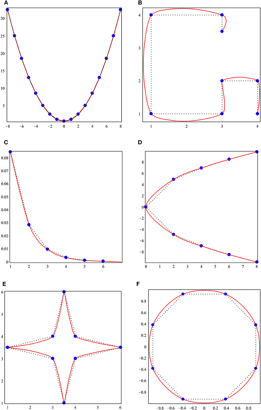
Figure 1. The convexity-preserving limit curves generated by the proposed scheme with the control polygon.

Now, we check whether the condition $\{d_i^j>0,i\in \mathbb{Z},j\in {\mathbb{N}}_0\}$ is satisfied by the four-point scheme (1) or not. By taking $y_i^j=\frac{d_{i+1}^j}{d_i^j},Y^j=max\{y_i^j,\frac{1}{y_i^j}\},j\in {\mathbb{N}}_0,i\in \mathbb{Z}$, we establish the following result.

Proposition 6.

For j ∈ ℕ, suppose that the initial control points $\left\{(x_i^0,p_i^0):i\in \mathbb{Z}\right\}$ are strictly convex, i.e., $d_i^0>0,i\in \mathbb{Z}$, such that

$\begin{array}{ll}{Y}^0\le \frac{1}{{\gamma }_i^{j+1}}={\delta }^j& (14)\end{array}$

then $d_i^j\le 0,$ i.e., the points generated by the four-point scheme (1) at the j^th subdivision step are not strictly convex.

Proof.

The second-order divided difference of the four-point scheme (1) can be obtained as:

$\begin{array}{l}\{\begin{array}{c}{d}_{3i}^{j+1}=\left(\frac{3}{2}{\gamma }_i^{j+1}+\frac{1}{20}\right)d_i^j+\left(\frac{3}{2}{\gamma }_i^{j+1}-\frac{1}{20}\right)d_{i+1}^j,\\ d_{3i+1}^{j+1}=\left(\frac{3}{2}{\gamma }_i^{j+1}-\frac{1}{20}\right)d_i^j+\left(\frac{3}{2}{\gamma }_i^{j+1}+\frac{1}{20}\right)d_{i+1}^j,\\ d_{3i+2}^{j+1}=\left(-\frac{3}{2}{\gamma }_i^{j+1}+\frac{1}{60}\right)d_i^j+\left(-3{\gamma }_i^{j+1}+\frac{3}{10}\right)d_{i+1}^j\\ +\left(-\frac{3}{2}{\gamma }_i^{j+1}+\frac{1}{60}\right)d_{i+2}^j.\end{array}\end{array}$

As ${\gamma }_i^{j+1}\in (1,\infty ),\forall j\in \mathbb{N}$, so it gives ${\delta }^j=\frac{1}{{\gamma }_i^{j+1}}>0.$ The proof of Proposition 6 proceeds by induction on j.

• By hypothesis, the assertion holds for j = 0, i.e., $d_i^0>0,Y^0\le {\delta }^j,i\in \mathbb{Z}.$

• Suppose by induction hypothesis $d_i^j>0$ and Y^j ≤ δ^j, i ∈ ℤ and for some j ∈ ℕ. Now we show that $d_i^{j+1}>0$. Also, simply, we have $\frac{1}{{\delta }^j}\le y_i^j\le {\delta }^j$ and $\frac{1}{{\delta }^j}\le \frac{1}{y_i^j}\le {\delta }^j$.

To prove $d_i^{j+1}>0$, it is sufficient to show that:

$\begin{array}{l}{d}_{3i}^{j+1}>0,d_{3i+1}^{j+1}>0\text{and }{d}_{3i+2}^{j+1}>0.\end{array}$

From (15), we have:

$\begin{array}{l}{d}_{3i}^{j+1}=\frac{3}{2}{\gamma }_i^{j+1}{d}_i^j+\frac{1}{20}{d}_i^j+\frac{3}{2}{\gamma }_i^{j+1}{y}_i^j{d}_i^j-\frac{1}{20}{y}_i^j{d}_i^j\\ >\frac{d_i^j}{60}[90{\gamma }_i^{j+1}+3+90{\gamma }_i^{j+1}\frac{1}{{\delta }^j}-3{\delta }^j]\\ =\frac{d_i^j}{60{\gamma }_i^{j+1}}[90{({\gamma }_i^{j+1})}^3+90{({\gamma }_i^{j+1})}^2+3({\gamma }_i^{j+1})-3].\end{array}$

As we know that $d_i^j>0$, and it is also clear that $\frac{1}{60{\gamma }_i^{j+1}}[90{({\gamma }_i^{j+1})}^3+90{({\gamma }_i^{j+1})}^2+3({\gamma }_i^{j+1})-3]>0$, for ${\delta }^j=\frac{1}{{\gamma }_i^{j+1}}$ and ${\gamma }_i^{j+1}>0$. So, we have:

$\begin{array}{ll}{d}_{3i}^{j+1}>0.& (15)\end{array}$

Now consider from (15)

$\begin{array}{l}{d}_{3i+1}^{j+1}=\left(\frac{3}{2}{\gamma }_i^{j+1}-\frac{1}{20}\right)d_i^j+\left(\frac{3}{2}{\gamma }_i^{j+1}+\frac{1}{20}\right)y_i^j{d}_i^j\\ >\frac{d_i^j}{60}\left(90{\gamma }_i^{j+1}-3+90{\gamma }_i^{j+1}\frac{1}{{\delta }^j}+3\frac{1}{{\delta }^j}\right)\\ =\frac{d_i^j{\gamma }_i^{j+1}}{60}\left(90-\frac{3}{{\gamma }_i^{j+1}}+90{\gamma }_i^{j+1}+3\right)\\ =\frac{d_i^j}{60}(90{({\gamma }_i^{j+1})}^2+93{\gamma }_i^{j+1}-3).\end{array}$

As we know that $d_i^j>0$, and it is clear that $\frac{1}{60}[90{({\gamma }_i^{j+1})}^2+93{\gamma }_i^{j+1}-3]>0$, for ${\delta }^j=\frac{1}{{\gamma }_i^{j+1}}$ and ${\gamma }_i^{j+1}>0$. This implies that:

$\begin{array}{ll}{d}_{3i+1}^{j+1}>0.& (16)\end{array}$

Now consider,

$\begin{array}{l}{d}_{3i+2}^{j+1}=\left(-\frac{3}{2}{\gamma }_i^{j+1}+\frac{1}{60}\right)d_i^j+\left(-3{\gamma }_i^{j+1}+\frac{3}{10}\right)d_i^j{y}_i^j\\ +\left(-\frac{3}{2}{\gamma }_i^{j+1}+\frac{1}{60}\right)d_i^j{y}_i^j{y}_{i+1}^j\\ >\frac{d_i^j}{60}(-90{\gamma }_i^{j+1}+1+\left(-180{\gamma }_i^{j+1}+\frac{1}{{\delta }^j}\right)\frac{1}{{\delta }^j}\\ +(18-90{\gamma }_i^{j+1}{\delta }^j)\frac{1}{{\delta }^j})\\ =\frac{d_i^j}{60}(-179{({\gamma }_i^{j+1})}^2-162{\gamma }_i^{j+1}+1),\end{array}$

As we know that $d_i^j>0$, and it is also clear that $\frac{d_i^j}{60}[-179{({\gamma }_i^{j+1})}^2-162{\gamma }_i^{j+1}+1]<0$, for ${\delta }^j=\frac{1}{{\gamma }_i^{j+1}}$ and ${\gamma }_i^{j+1}>0$. This implies that:

$\begin{array}{ll}{d}_{3i+2}^{j+1}<0.& (17)\end{array}$

By combining (15), (16), and (17), we have $d_i^{j+1}\le 0$, which shows that the four-point scheme (1) does not preserve strict convexity. Some numerical examples are presented to verify and examine the conditions of shape preserving for the 4-point ternary scheme (1). In Examples 1 − 4, the initial set of values is displayed by dotted line segments while the limit curves are marked by solid lines, such that the limit curves generated by the four-point scheme (1) satisfy the shape-preserving condition.

Example 1.

There are several important meteorological data parameters that scientists use for dealing with different climate challenges. Wind velocity data (WVD) is one of them. These data always have a positive value, and the minimum value is ~0. In this example, we choose WVD from Wu et al. [23], as given in Table 1. We use these WVD to demonstrate the positivity-preserving property of the four-point scheme (1). In Figure 2A, the dotted line represents WVD (which is positive) and the solid curve is generated by the four-point scheme (1), which is also positive.

TABLE 1

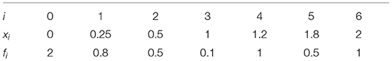
Table 1. Wind data (positive data) [23].

FIGURE 2

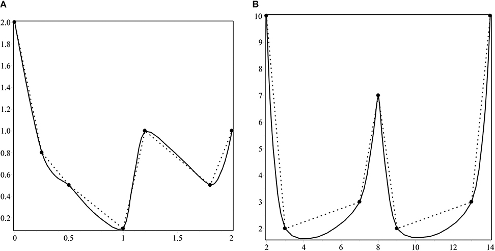
Figure 2. The positivity-preserving curves generated by the four-point scheme (1) for positive initial data.

Example 2.

In this example, we consider experimental data that are quoted from Sarfraz et al. [24]. The proposed data are positive and represent the volume of NaOH vs. HCl in a beaker, as stated in the experimental procedures. These experimental data are presented in Table 2. Figure 2B presents the positivity preservation of the curve generated by the four-point scheme (1). In this figure, the dotted line represents the positive data (which are given in Table 2) and the solid curve is generated by the four-point scheme (1). It is clear that the curve generated by the scheme is also positive.

TABLE 2

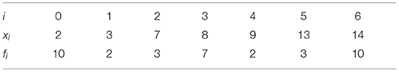
Table 2. Positive data from Sarfraz et al. [24].

Example 3.

The data given in Table 3 are also experimental data. These data represent the oxygen level from an experiment conducted in the laboratory and are quoted from Butt and Brodlie [25]. We use the proposed data in Figure 3A. In this figure, we find that, by imposing the condition of positivity on the initial data, the four-point scheme (1) is capable of producing a positive curve.

TABLE 3

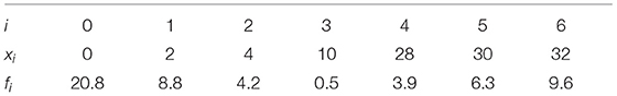
Table 3. Positive data from Butt and Brodlie [25].

FIGURE 3

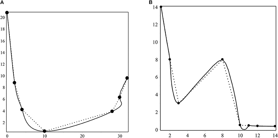
Figure 3. The positivity-preserving curves generated by the four-point scheme (1) for positive initial data.

Example 4.

The data in Table 4 are obtained from Hussain and Ali [26]. These data represent the depreciation of the valuation of the market price of computers installed at City Computer Center. The x-coordinate corresponds to the time in years, and the y-coordinate corresponds to the computer price in Rs. 10,000. Figure 3B generated by the four-point scheme (1) indicates the positivity preservation of the curve generated by the scheme.

TABLE 4

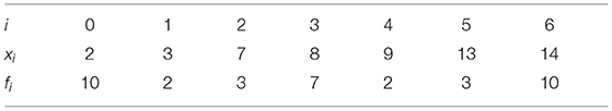
Table 4. Positive data from Hussain and Ali [26].

Example 5.

The data given in Table 5 represents monotonic data that are obtained from a monotonic function. From Figure 4A we find that by imposing the condition of monotonicity on the initial data, the four-point scheme (1) is capable of producing a monotonically increasing curve.

TABLE 5

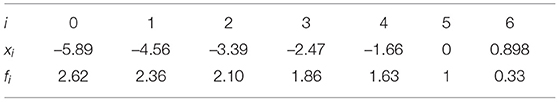
Table 5. Monotonic data.

FIGURE 4

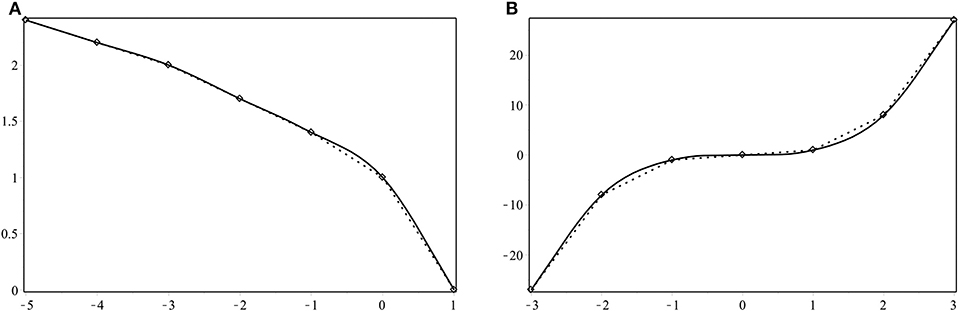
Figure 4. The monotonicity-preserving curves generated by the four-point scheme (1) with monotonic initial data.

Example 6.

In this example, we again consider monotonic data from a monotonic function. These data are presented in Table 6. Figure 4B displays the curve generated by the four-point scheme (1). It is clear from the figure that, for an initial monotonic dataset, the scheme produces a monotonic curve.

TABLE 6

Table 6. Monotonic data.

6. Conclusion

In this paper, we have presented the shape-preserving properties of the four-point scheme (1). We have derived the necessary conditions on the initial control points and tension parameter of the scheme to show that the four-point scheme (1) generates positivity- and monotonicity-preserving curves after a finite number of subdivision steps. We have also shown that, for initial convex data, the proposed scheme does not generate a convex curve. Further, we have generalized these results for the positivity- and monotonicity-preservation of the limit curves. Finally, the discussion is followed by several numerical examples. By using this technique, one can analyze the shape-preserving properties of higher arity interpolation and also approximating schemes.

Data Availability Statement

All datasets generated for this study are included in the article/supplementary files.

Author Contributions

PA, AG, and KN: conceptualization. PA, MS, AG, and KN: writing the original manuscript: MS and IK: formal analysis: IK: methodology and supervision: KN and IK: writing review and editing: PA, MS, AG, KN, and IK: software.

Conflict of Interest

The authors declare that the research was conducted in the absence of any commercial or financial relationships that could be construed as a potential conflict of interest.

References

1. Kanwal G, Ghaffar A, Hafeezullah MM, Manan SA, Rizwan M, Rahman G. Numerical solution of 2-point boundary value problem by subdivision scheme. Commun Math Appl. (2019) 10:1–11. doi: 10.26713/cma.v10i1.980

CrossRef Full Text | Google Scholar

2. Tassaddiq A, Khalid A, Naeem MN, Ghaffar A, Khan F, Karim SAA, et al. A new scheme using Cubic B-Spline to solve non-linear differential equations arising in visco-elastic flows and hydrodynamic stability problems. Mathematics. (2019) 7:1078. doi: 10.3390/math7111078

CrossRef Full Text | Google Scholar

3. Goufo EFD, Kumar S, Mugisha SB. Similarities in a fifth-order evolution equation with and with no singular kernel. Chaos Solit Fractals. (2020) 130:109467. doi: 10.1016/j.chaos.2019.109467

CrossRef Full Text | Google Scholar

4. Zaid O, Kumar S. A robust computational algorithm of homotopy asymptotic method for solving systems of fractional differential equations. J. Comput. Nonlinear Dynam. (2019) 14:081004. doi: 10.1115/1.4043617

CrossRef Full Text | Google Scholar

5. Ahmad E, Oqielat MN, Al-Zhour Z, Kumar S, Momani S. Solitary solutions for time-fractional nonlinear dispersive PDEs in the sense of conformable fractional derivative. Chaos Interdiscip J Nonlinear Sci. (2019) 29:093102. doi: 10.1063/1.5100234

CrossRef Full Text | Google Scholar

6. Kumar S, Kumar A, Momani S, Aldhaifallah M, Nisar KS. Numerical solutions of nonlinear fractional model arising in the appearance of the stripe patterns in two-dimensional systems. Adv Diff Equ. (2019) 2019:413. doi: 10.1186/s13662-019-2334-7

CrossRef Full Text | Google Scholar

7. Sharma B, Kumar S, Cattani C, Baleanu D. Nonlinear dynamics of Cattaneo-Christov heat flux model for third-grade power-law uid. J Comput Nonlinear Dynam (2019) 15:9. doi: 10.1115/1.4045406

CrossRef Full Text | Google Scholar

8. de Rham G. Sur une courbe plane. J de Mathmat Pures et Appl. (1956) 35:25–42.

Google Scholar

9. Chaikin GM. An algorithm for high-speed curve generation. Comput Graph Image Proc. (1974) 3:346–9.

Google Scholar

10. Dyn N, Levin D, Gregory JA. A 4-point interpolatory subdivision scheme for curve design. Comput Aided Geom Des. (1987) 4:257–68.

Google Scholar

11. Dyn N, Kuijt F, Levin D, van Damme R. Convexity preservation of the four-point interpolatory subdivision scheme. Comput Aided Geom Des. (1999) 16:789–92.

Google Scholar

12. Kuijt F, van Damme R. Monotonicity preserving interpolatory subdivision schemes. J Comput Appl Math. (1999) 101:203–29.

Google Scholar

13. Beccari C, Casciola G, Romani L. Shape controlled interpolatory ternary subdivision. Appl Math Comput. (2009) 215:916–27. doi: 10.1016/j.amc.2009.06.014

CrossRef Full Text | Google Scholar

14. Hassan MF, Ivrissimitzis IP, Dodgson NA, Sabin MA. An interpolating 4-point C² ternary stationary subdivision scheme. Comput Aided Geom Des. (2002) 19:1–18. doi: 10.1016/S0167-8396(01)00084-X

CrossRef Full Text | Google Scholar

15. Cai Z. Convexity preservation of the interpolating four-point C² ternary stationary subdivision scheme. Comput Aided Geom Des. (2009) 26:560–65. doi: 10.1016/j.cagd.2009.02.004

CrossRef Full Text | Google Scholar

16. Pitolli F. Ternary shape-preserving subdivision schemes. Math Comput Simul. (2014) 106:185–94. doi: 10.1016/j.matcom.2013.04.003

CrossRef Full Text | Google Scholar

17. Beccari C, Casciola G, Romani L. A non-stationary uniform tension controlled interpolating 4-point scheme reproducing conics. Comput Aided Geom Des. (2007) 24:1–9. doi: 10.1016/j.cagd.2006.10.003

CrossRef Full Text | Google Scholar

18. Akram G, Bibi K, Rehan K, Siddiqi SS. Shape preservation of 4-point interpolating non-stationary subdivision scheme. J Comput Appl Math. (2017) 319:480–92. doi: 10.1016/j.cam.2017.01.026

CrossRef Full Text | Google Scholar

19. Beccari C, Casciola G, Romani L. An interpolating 4-point C² ternary non-stationary subdivision scheme with tension control. Comput Aided Geom Des. (2007) 24:210–19. doi: 10.1016/j.cagd.2007.02.001

CrossRef Full Text | Google Scholar

20. Ghaffar A, Ullah Z, Bari M, Nisar KS, Baleanu D. Family of odd point non-stationary subdivision schemes and their applications. Adv Diff Equ. (2019) 2019:171. doi: 10.1186/s13662-019-2105-5

CrossRef Full Text | Google Scholar

21. Ghaffar A, Bari M, Mudassar I, Nisar KS, Baleanu D. A new class of 2q-point nonstationary subdivision schemes and their applications. Mathematics. (2019) 7:639. doi: 10.3390/math7070639

CrossRef Full Text | Google Scholar

22. Ghaffar A, Ullah Z, Bari M, Nisar KS, Qurashi AL, Baleanu D. A new class of 2m-point binary non-stationary subdivision schemes. Adv Diff Equ. (2019) 2019:325. doi: 10.1186/s13662-019-2264-4

CrossRef Full Text | Google Scholar

23. Wu J, Zhang X, Peng L. Positive approximation and interpolation using compactly supported radial basis functions. Math Problem Eng. (2010) 10:964528. doi: 10.1155/2010/964528

CrossRef Full Text | Google Scholar

24. Sarfraz M, Hussain MZ, Nisar A. Positive data modeling using spline function. Appl Math Comput. (2010) 216:2036–49. doi: 10.1016/j.amc.2010.03.034

CrossRef Full Text | Google Scholar

25. Butt S, Brodlie KW. Preserving positivity using piecewise cubic interpolation. Comput Graph. (1993) 17:55–64.

Google Scholar

26. Hussain MZ, Ali JM. Positivity preserving piecewise rational cubic interpolation. Matematika. (2006) 22:147–53. doi: 10.11113/matematika.v22.n.183

CrossRef Full Text | Google Scholar