On the Time Shift Phenomena in Epidemic Models

1. Introduction

From the early attempts [1–4] to recent studies, epidemic modeling which is applicable in a wide range of fields from informatics [56] to chemistry [7–9] has drawn the attention of researchers in various disciplines. Since the basic compartmental model Susceptible-Infected-Removed (SIR) which is commonly used to model diseases for which the infection confers permanent immunity was introduced by Kermack and McKendrick in 1927 [4]; other compartmental models [10–12] have been developed to model diseases with different structures and dynamics. Especially in recent years, major outbreaks such as avian flu in 2005, swine influenza in 2006, and H1N1 influenza in 2009 have highlighted the need for more effective and reliable models to control the spread of disease and to provide a better knowledge for the prediction of future threats and for the development of stronger containment strategies. In Refs. [13–18], some results on the modeling of different types of epidemic diseases, the solution form of these models, the observation of global stability, and the determination of the final size of the epidemic are obtained. In Ref. [15], global stability criteria are derived for the SEIS model which can be regarded as a model with no immunity, and different SIR models are examined in Refs. [1617]. Moreover, the works [1718] provide some useful results on the final size of the epidemic for SIR models. With the same motivation of these works but rather a different contribution to literature, we use a multistage model [14] in this article to explain the time shift observed in several surveys such as Spanish flu (1918–1919) [19], SARS (2002–2004), the 2009 H1N1 in Istanbul, and recently, COVID-19 [20] (see Figures 1–3).

FIGURE 1

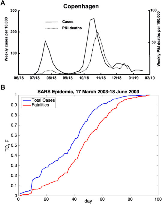
FIGURE 1. (A) Weekly number of influenza cases and respiratory deaths (pneumonia and influenza) in Copenhagen, Denmark, during 1918–1919 are presented. This figure was taken from the study of Andreasen et al. [19] (copyright Andreasen et al. [19]). A shift occurred between the maxima of curves. (B) Daily number of total cases and cumulative number of the fatalities for the 2003 SARS epidemic in the world are shown. The data provided by WHO were used in the generation of this figure (https://www.who.int/csr/sars/country/en/) (last access: September 15, 2020). An explicit shift was also observed for the SARS epidemic.

FIGURE 2

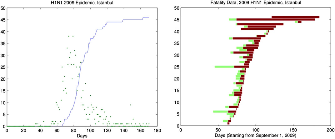
FIGURE 2. Daily number of referrals to hospitals and cumulative number of fatalities for the 2009 H1N1 epidemic in Istanbul, Turkey. The scatter in the number of daily referral to hospitals indicates that the hospitalization rate varies during the epidemic. The asymmetry of the incidence curve is still observable. The fatalities shown here are adjusted to at most 15 days after referral to the hospital (left panel). The duration of symptoms prior to hospitalization (light color) and the duration of hospitalization prior to death (dark color) for the fatalities in Istanbul, Turkey, due to 2009 H1N1 epidemic (right panel).

FIGURE 3

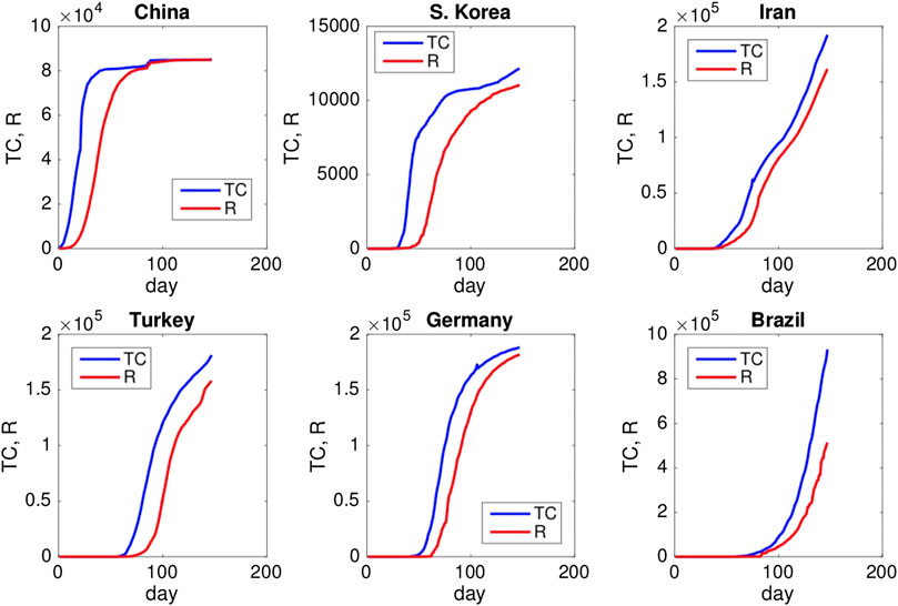
FIGURE 3. Graphs of total cases (TC) and removed individuals (R) for selected countries. The dataset of each country is collected according to published official reports and available at the website http://www.worldometers.info/coronavirus/ (last access: June 28, 2020). Updated data are also available at the website http://epikhas.khas.edu.tr/. The last data in this work were collected on the 16th of June 2020. Data cover the period January 22–June 28, 2020, and in the following, “Day 1” corresponds to January 22, 2020.

In the literature, available observed data that are used for the ordinary differential equation system representing the classical SIR epidemic model is based on the curve of removed individuals. Usually, this curve is obtained by taking into consideration only the fatality data of the epidemic disease, whereas in some research studies, not only the fatality data but also the hospitalization data for the epidemic are taken into account in the modeling process. In Ref. [21], it is shown that there exists a delay between the peak of the hospitalization (infectious) curve and the inflection point of the fatality (removed) curve based on the data collected. The original contribution of this article to the literature is that we explain this time shift by the multidimensional form of SIR and SEIR models and also provide numerical evidence that the expected delay is approximately half of the infectious period of the epidemic disease for both of the multistage systems.

In the second section of this work, we give a brief summary of the classical epidemic SIR and SEIR models and define the multistage form of these models that will be used in further analysis. The graphs obtained by the numerical evaluations of the classical SIR and SEIR models and their multistage forms are also given. Analysis of these graphs confirms that the multistage SIR and SEIR models explain the time shift observed in several surveys. In the third section, the evaluation of delay for different epidemic parameters is presented by using the numerical evaluations of these multistage models. In the fourth section, the distance between the points where successive stages and hence any two stages assume their maximum is found approximately. The last section includes a summary of the results obtained in the previous sections as well as motivations for future analysis.

2. Standard Epidemic Models and Epidemic Models With Multiple Infectious Stages

The SIR model is commonly used to model diseases for which the removed individuals are assumed to be immune to reinfection. In addition, the total population with constant size is divided into three distinct compartments the size of which change with time t. These compartments are called the susceptible class S, the infective class I, and the removed class R. Healthy individuals with no immunity are members of class S until they are infected with a pathogen and become capable of transmitting the disease to others. They move from the class S into the class I once they are infected and then from I to R once they recover or die. Childhood illnesses like measles or rubella are good examples for the SIR model.

The SIR epidemic model without vital dynamics, that is, the recruitment of new susceptible through birth or immigration as well as the loss through mortality or emigration are ignored, is defined by the following system of nonlinear ordinary differential equations:

$\begin{array}{c}SIR:S^{\prime }=-\beta SI,\\ I^{\prime }=\beta SI-\gamma I,\\ R^{\prime }=\gamma I,\end{array}(1)$

where the coefficient β refers to the disease transmission rate and $1/\gamma$ represents the duration of infection period. Note that since $S^{\prime }+I^{\prime }+R^{\prime }=0$, we may assume $S+I+R=1$ by the use of appropriate normalization.

The standard SIR model ignores a latent phase which is the delay between the time of the acquisition of infection and the onset of infectiousness. In order to define this latent phase, the introduction to the SIR model of an exposed class E whose members are individuals who have been infected with a pathogen but are not yet infectious due to the incubation period of pathogen yields the SEIR model. Chicken pox is suitable for the SEIR model, which is defined by the following system of ordinary differential equations

$\begin{array}{c}SEIR:S^{\prime }=-\beta SI,\\ E^{\prime }=\beta SI-\mathrm{ϵ}E,\\ I^{\prime }=\mathrm{ϵ}E-\gamma I,\\ R^{\prime }=\gamma I,\end{array}(2)$

where $1/\mathit{ϵ}$ represents the mean exposed period. Note that we may assume $S+E+I+R=1$ by the use of appropriate normalization.

These two models are suitable for mathematical modeling of seasonal diseases, but they fail to reproduce the time shift that was observed in the modeling of the 2009 H1N1 epidemic in Istanbul, Turkey [21], as shown in Figure 2. For COVID-19, a similar time shift is observed between the curves of total cases and removed individuals in China, South Korea, Iran, Turkey, Germany, and Brazil as shown in Figure 3. Publicly accessible data that have been released by the state offices of each country are used for this analysis.

In the literature, a similar time shift is also observed for Spanish flu [19] and SARS epidemics. The graphs for the data of these epidemics are shown in Figure 1. Weekly case and fatality reports for Copenhagen, Denmark, in 1918–1919 are displayed in Figure 1A. In this figure, it can clearly be seen that there is a time shift between the peak of the infectious cases and the peak of fatalities. Similarly, in Figure 1A–B, the time shift is also observable between cumulative cases and cumulative fatalities.

In this study, we use multiple infectivity periods [1314] to explain this delay that is unforeseen in the standard SIR model. The approach of multiple infectious stages consists of replacing the single infectious stage I with $N+1$ substages denoted by $I_i$, which is the density of individuals in the ith infectious stage. Unlike the model in Ref. [14], each of these stages may have different infectivity ${\beta }_i$ and a variable infectious period $1/{\gamma }_i$. In order to compare the solution curves with the ones for the standard SIR and SEIR models, we set

$\frac{1}{{\gamma }_0}+\frac{1}{{\gamma }_1}+\cdots +\frac{1}{{\gamma }_N}=\frac{1}{\gamma }.$

The multistage SIR and SEIR epidemic models are defined by the following systems:

$\begin{array}{c}MultistageSIR:S^{\prime }=-S\left({\beta }_0{I}_0+{\beta }_1{I}_1+\cdots +{\beta }_N{I}_n\right)\text{,}\\ {I^{\prime }}_0=S({\beta }_0{I}_0+{\beta }_1{I}_1+\cdots +{\beta }_n{I}_N)-{\gamma }_0{I}_0\text{,}\\ {I^{\prime }}_1={\gamma }_0{I}_0-{\gamma }_1{I}_1\text{,}\\ \cdots \cdots \cdots \\ \cdots \cdots \cdots \\ {I^{\prime }}_N={\gamma }_{N-1}{I}_{N-1}-{\gamma }_N{I}_N\text{,}\\ R^{\prime }={\gamma }_N{I}_N\text{,}\end{array}(3)$

$\begin{array}{c}MultistageSEIR:S^{\prime }=-S\left({\beta }_1{I}_1+\cdots +{\beta }_N{I}_N\right),\\ E^{\prime }=S({\beta }_1{I}_1+\cdots +{\beta }_N{I}_N)-\mathrm{ϵ}E,\\ {I^{\prime }}_1=\mathrm{ϵ}E-{\gamma }_1{I}_1\text{,}\\ {I^{\prime }}_2={\gamma }_1{I}_1-{\gamma }_2{I}_2\text{,}\\ \cdots \cdots \cdots \\ \cdots \cdots \cdots \\ {I^{\prime }}_N={\gamma }_{N-1}{I}_{N-1}-{\gamma }_N{I}_N,\\ R^{\prime }={\gamma }_N{I}_N.\end{array}(4)$

The multistage SIR and SEIR systems with ${\beta }_0=\dots ={\beta }_n$ and ${\gamma }_0=\dots ={\gamma }_n$ correspond to the choice of gamma-distributed “Infection Period Distribution” (IPD) in the integral equation formulation of the SIR model [14].

The linear parts of apparently different infectious stages for $i\ge 1$ in the multistage SIR model and $i\ge 2$ in the multistage SEIR model have a similar structure. We write the linear parts of each equation above as a system and then rearrange and rename as follows to keep the models as clear and simple as possible

$\begin{array}{l}SJR:J=I_0+\frac{{\beta }_1}{{\beta }_0}{I}_1+\cdots +\frac{{\beta }_N}{{\beta }_0}{I}_N\text{,}\\ S^{\prime }=-{\beta }_{0}SJ\text{,}\\ {I^{\prime }}_0={\beta }_{0}SJ-{\gamma }_0{I}_0\text{,}\\ {I^{\prime }}_i={\gamma }_{i-1}{I}_{i-1}-{\gamma }_i{I}_i,\hspace{1em}fori=1,\dots N\text{,}\\ R^{\prime }={\gamma }_N{I}_N,\end{array}(5)$

$\begin{array}{l}SEJR:J=I_1+\frac{{\beta }_2}{{\beta }_1}{I}_2\cdots +\frac{{\beta }_N}{{\beta }_1}{I}_N\text{,}\\ S^{\prime }=-{\beta }_{1}SJ\text{,}\\ E^{\prime }={\beta }_{1}SJ-\mathrm{ϵ}E\text{,}\\ {I^{\prime }}_1=\mathrm{ϵ}E-{\gamma }_1{I}_1\text{,}\\ {I^{\prime }}_i={\gamma }_{i-1}{I}_{i-1}-{\gamma }_i{I}_i,\hspace{1em}fori=2,\dots N\text{,}\\ R^{\prime }={\gamma }_N{I}_N.\end{array}(6)$

Subsequently, the numerical evaluations of these two systems, SJR and SEJR, defined above will be used for some of the structural comparisons of the classical models and multistage models. A MATLAB^® ODE45 solver is used for all the numerical evaluations. In typical cases, initial conditions are chosen so that $S\left(0\right)$ is close to 1, whereas $E\left(0\right)$ and $I_i\left(0\right)$ are close to zero, and $R\left(0\right)$ is chosen so that the sum of all variables is 1, that is,

$S\left(0\right)=1-{10}^{-4},I_0\left(0\right)={10}^{-4},I_i\left(0\right)=0,i=1,\dots .,N,R\left(0\right)=0;(7)$

and for the SEJR model,

$S\left(0\right)=1-{10}^{-4},E\left(0\right)=5\times {10}^{-5},I_1\left(0\right)=5\times {10}^{-5},I_i\left(0\right)=0,i=2,\dots .,N,R\left(0\right)=0.(8)$

Numerical evaluations of the classical SIR and SEIR models are made for specific epidemic parameters, and the results are given in Figure 4. For the evaluations of the classical models, γ and ϵ are fixed as $1/5$ and $1/3$, respectively, whereas the value of $R_0$ is chosen to be 2.5 and 10, respectively. In all cases, the maximum of the infectious stage and the inflection point of the removed stage occur at the same point in time; hence, there is no time shift in these classical models.

FIGURE 4

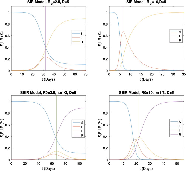
FIGURE 4. Numerical solutions of classical SIR (1) and SEIR (2) models with $R_0=2.5$ and 10. Here, ϵ and γ are chosen as $1/3$ and $1/5$ ($D=5$), respectively. Time shift does not occur in classical models.

Numerical evaluations of the multistage SIR model are repeated for various stage numbers. First, $R_0$ is set as 2.5, while the total number of stages, N, is given the values $\mathrm{5,10,30}$, and 60, and the corresponding graphs of the solutions are shown in Figure 5. In these evaluations, ${\gamma }_i$ is chosen to be $0.2\times N$, for $i=\mathrm{0,1},\dots ,N$. In Figure 5, the time shift between the maximum point of the curve, representing the sum of the infectious stages, $J\left(t\right)$ and the inflection point of $R\left(t\right)$ can clearly be seen. As predicted, the system given by Eq. 5 confirms the delay and therefore seems adequate to explain the time shift between infectious and removed stages observed in Istanbul data [21]. Note that the time shifts for $N=\mathrm{10,30,60}$ seem to be equal but the one for $N=5$ is smaller.

FIGURE 5

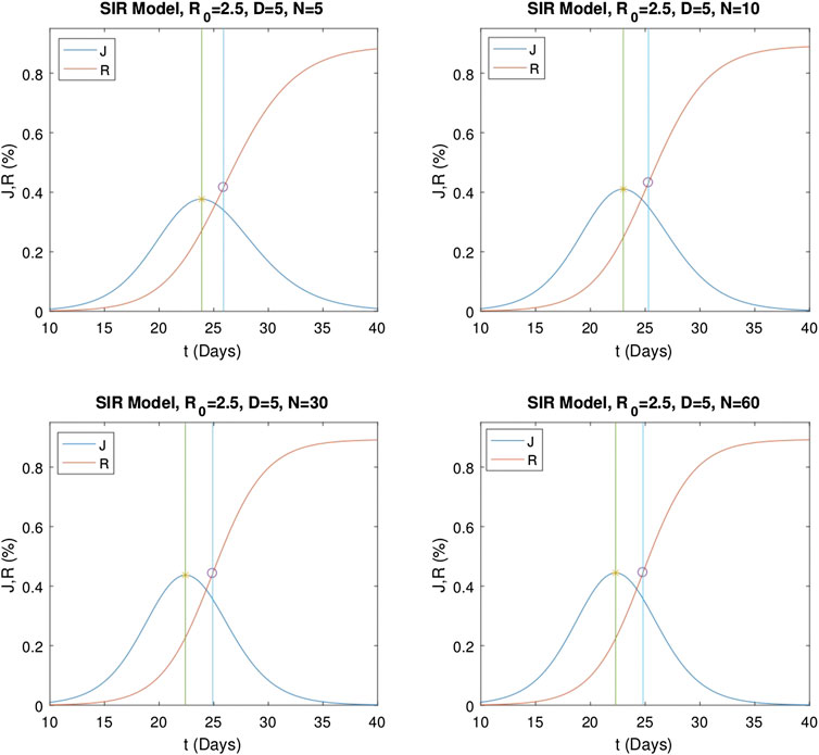
FIGURE 5. Numerical solutions of the multistage SIR model for different stage numbers $N=\mathrm{5,10,30}$, and 60. Here, $R_0=2.5$ and $\gamma =0.2\times N$. In the graphs, $\text{*}$ represents the location of the maximum value of J and o represents the location of the inflection point of R. Graphs show that there is a time shift between these points.

Similarly, numerical evaluations of the multistage $SEIR$ model are obtained for various stage numbers. First, $R_0$ is set as five, while the stage number N is given the values $\mathrm{5,10,30}$, and 60, and the corresponding graphs of the solutions are shown in Figure 6. In these evaluations, ϵ and ${\gamma }_i$ are chosen to be $1/3$ and $0.2\times N$, respectively, for $i=1,\dots ,N$. Figure 6 illustrates that just like it is seen in the SJR system, there exists a time shift between the maximum point of J and the inflection point of R in the SEJR model, with characteristics similar to the ones for the SIR model.

FIGURE 6

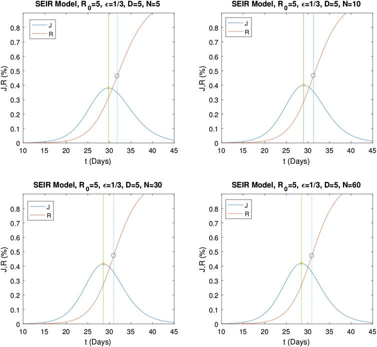
FIGURE 6. Numerical solutions of the multistage SEIR model for different stage numbers $N=\mathrm{5,10,30}$, and 60. Here, $R_0=2.5$, $\mathit{\epsilon }=1/3$, and $\gamma =0.2\times N$. In the graphs, $\text{*}$ represents the location of the maximum value of J and o represents the location of the inflection point of R. Graphs show that there is a time shift between these points.

3. Numerical Results for Models With Multiple Infectious Stages

In this section, we investigate the dependency of the delay on the epidemic parameters by numerical evaluations of system Eq. 5. Graphs $I{(}_i(t)$ for $N=\mathrm{1,2,3,4}$ for the SIR and SEIR models are given in Figures 7 and 8, respectively. To analyze the nature of the time shift for relatively large values of the stage number, the graphs of the solutions for the same epidemic parameters are obtained for N ranging from 2 to 16 in steps of two and the corresponding graphs are given in Figure 9. As it can be seen from Figure 9, the solution curves start to resemble as the stage number N increases. Finally, in Figure 10, we present the dependency of the time shift on the number of stages N, for $1\le N\le 150$. Similar computations are repeated for the SEIR model and the results are presented in Figures 11, 12.

FIGURE 7

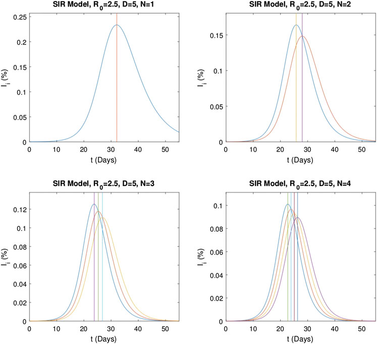
FIGURE 7. Graphs of the independent infectious stages $I_0,\dots I_N$ from numerical solutions of the multistage SIR model (5). Here, $R_0=2.5$ and $\gamma =0.2\times N$. In the graphs, vertical lines indicate the position of maximum points of the independent infectious stages. The distance between these vertical lines is approximately $1/\gamma$.

FIGURE 8

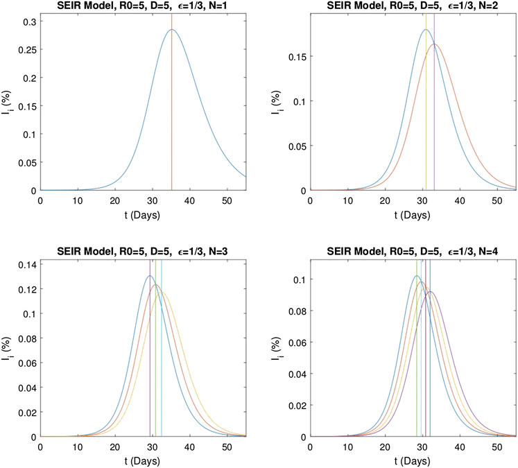
FIGURE 8. Graphs of the independent infectious stages $I_1,\dots I_N$ from numerical solutions of the multistage SEIR model (6). Here, $R_0=2.5$, $\mathit{\epsilon }=1/3$, and $\gamma =0.2\times N$. In the graphs, vertical lines indicate the position of maximum points of the independent infectious stages. The distance between these vertical lines is approximately $1/\gamma$.

FIGURE 9

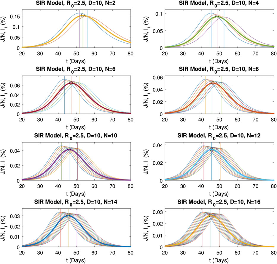
FIGURE 9. Change of the position of maximum of $J/N$ (normalized J) in time with respect to the number of stages N for the multistage SIR model. “o” indicates the position of the maxima of $J/N$ (thick curves). Vertical lines represent the position of maximum points of the first stage, $J/N$, and the last stage, respectively.

FIGURE 10

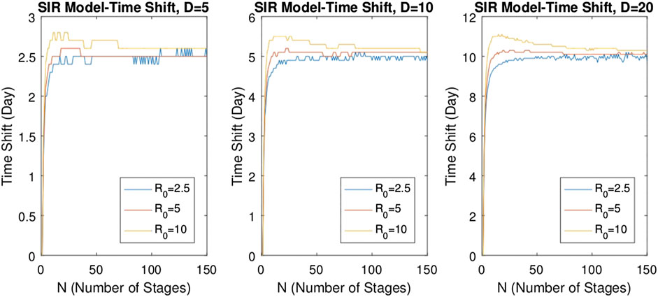
FIGURE 10. Variations of time shift (delay) with respect to the number of stages N for $R_0=2.5,5$, and 10; $D=5,10$, and 20 in the multistage SIR model. For all cases, the time shift becomes stable at a constant value after a critical stage number N.

FIGURE 11

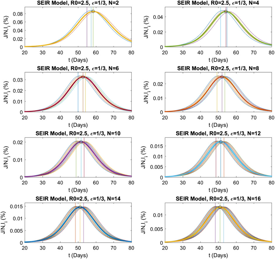
FIGURE 11. Change of the position of maximum of $J/N$ (normalized J) in time with respect to the number of stages N for the multistage SEIR model. “o” indicates the position of the maxima of $J/N$ (thick curves). Vertical lines represent the position of maximum points of the first stage, $J/N$, and the last stage, respectively.

FIGURE 12

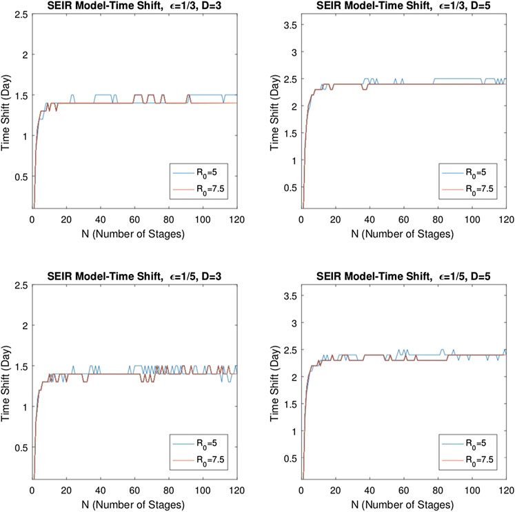
FIGURE 12. Variation of time shift for $R_0=5$ and 7.5 in the multistage SEIR model. Here, $\mathit{ϵ}=1/3,1/5$, and $D=3,5$ are taken. For each case, delay becomes stable at a constant value after a critical stage number N.

For the SIR model, to investigate the effect of the basic reproduction number $R_0$ and the infectious period $1/\gamma$ on the infectious dynamics and the resulting delay, system (5) is solved with the initial conditions given by Eq. 7 for some parameter values. To this end, the pair $\left(R_0,1/\gamma \right)$ is chosen $\left(2.5,5\right)$, $\left(\mathrm{5,5}\right)$, $\left(\mathrm{10,5}\right)$, $\left(2.5,10\right)$, $\left(\mathrm{5,10}\right)$, $\left(\mathrm{10,10}\right)$, $\left(2.5,20\right)$, $\left(\mathrm{5,20}\right)$, and $\left(\mathrm{10,20}\right)$, respectively, and the numerical evaluations for various infectious stages N are shown in Figure 10. It can be observed from this figure that the delay is almost half of the infectious period. This fact can also be seen in Figure 9 where the time value of the maximum of $J/N$ (normalized J) in time is located at the middle of time values of the maximum of the first infectious stage and the maximum of the last infectious stage. Comparison of panels of Figure 10 shows that the change in the reproduction number $R_0$ for a fixed infection period has no effect on the delay. On the other hand, the delay depends on the infection period; in fact, it is approximately half of it for large N.

The same analysis is repeated for the multistage SEIR model. The system defined by Eq. 6 is solved for the same epidemic parameters and initial conditions as above and with $\mathit{\epsilon }=1/3$, and the resulting graphs are given in Figure 11. As for the SIR model, the solution curves start to resemble for large N and the peak of $J\left(t\right)$ is located at the midpoint of the delay interval.

To illustrate the dependency of the delay on the system parameters of the $SEIR$ model, the pairs $\left(\mathit{\epsilon },\gamma \right)$ are chosen as $(1/\mathrm{3,1}/3)(1/3,(1/5),(1/\mathrm{5,1}/3),(1/\mathrm{5,1}/5)$, and variations of the delay for each of these cases are presented in Figures 12A–D, for $R0=5$ and $R0=7.5$. An analysis of these graphs yields that as N increases, the delay converges to a value. Moreover, it could easily be observed that the delay is independent of ϵ and $R_0$, but yet it is influenced by $1/\gamma$ (i.e., infectious period). Note that the delay for the multistage SEIR model is shorter than the delay observed in the multistage SIR model.

4. Estimation of the Delay

In this section, we use a quadratic approximation to each $I_i\left(t\right)$ around the peak of $I_{i-1}\left(t\right)$ to show that within the validity of the quadratic approximation, the delays between successive peaks are $1/{\gamma }_i$.

Let $t_i$ be the time where each $I_i$ assumes its maximum and $1/{\gamma }_i$ be the corresponding infectious period for $i=\mathrm{0,1},\dots N$. To determine the distance between the points $t_i$ where each substage $I_i$ assumes its maximum value, we use quadratic approximation of the Taylor series expansion of $I_i$ at the point $t=t_{i-1}$ where,

$I_i\left(t\right)=I_i\left(t_{i-1}\right)+I_i^{\prime }\left(t_{i-1}\right)(t-t_{i-1})+\frac{1}{2}{I}_i^{\prime \prime }\left(t_{i-1}\right){(t-t_{i-1})}^2,(9)$

for $i\ge 1$. Differentiating

$I_i^{\prime }\left(t\right)=I_i^{\prime }\left(t_{i-1}\right)+I_i^{\prime \prime }\left(t_{i-1}\right)\left(t-t_{i-1}\right)(10)$

and then substituting $t=t_i$ in Eq. 10 and using the fact that $I_i^{\prime }\left(t_i\right)=0$ since $I_i$ reaches its maximum at $t_i$, one obtains

$t_i-t_{i-1}=-\frac{I_i^{\prime }\left(t_{i-1}\right)}{I_i^{\prime \prime }\left(t_{i-1}\right)}.(11)$

The multistage SIR model defined by the equations in Eq. 5 suggests that for $i\ge 1$,

$I_i^{\prime }\left(t\right)={\gamma }_{i-1}{I}_{i-1}\left(t\right)-{\gamma }_i{I}_i\left(t\right).(12)$

Differentiating Eq. 12 yields

$I_i^{\prime \prime }\left(t\right)={\gamma }_{i-1}{I}_{i-1}^{\prime }\left(t\right)-{\gamma }_i{I}_i^{\prime }\left(t\right).(13)$

By considering the fact that $I_{i-1}^{\prime }\left(t_{i-1}\right)=0$ since $I_{i-1}$ assumes its maximum value at $t_{i-1}$, one gets the following by replacing $t=t_{i-1}$ in equation

$I_{i-1}^{\prime \prime }\left(t_{i-1}\right)=-{\gamma }_i{I}_i^{\prime }\left(t_{i-1}\right).$

Substitution of the equation above in Eq. 11 gives the approximate distance formula as follows:

$t_i-t_{i-1}=\frac{1}{{\gamma }_i}.(14)$

Therefore, the distance between any $t_i$ is $t_i-t_j=\stackrel{i}{{\displaystyle \sum }_{k=j+1}}\frac{1}{{\gamma }_k}$.

Results obtained by the numerical evaluations are compatible with Eq. 14. To observe the distance between the maximum points of the independent infectious stages, solutions of the multistage SIR model with respect to various infectious periods are chosen. In this respect, the basic reproduction numbers $R_0$ and ${\gamma }_i$ (i.e., duration is 5) are set as 2.5 and $0.2\times N$, respectively, and the related graphs of the solutions for various stage numbers ($N=\mathrm{1,2,3,4}$) are given in Figure 7. Comparison of graphs in Figure 7 reveals that the value of the difference of the points where successive stages reach their maximum is approximately $1/{\gamma }_i$.

It should be emphasized that Eq. 14 is also valid for the multistage SEIR model. The distance between the maximum points of the independent infectious stages including the E stage is approximately $1/{\gamma }_i$. Since the proof is the same as in the SIR case, we do not repeat the derivation of Eq. 14 again to avoid repetition. However, to observe the distance between the maximum points of the infectious stages numerically, the basic reproduction numbers $R_0$, ϵ, and ${\gamma }_i$ (i.e., duration is 5) are set as 5, $1/3$, and $0.2\times N$. Then, the SEIR model is solved for $N=\mathrm{1,2,3}$, and 4, and the related graphs are given in Figure 8. As in the case of the SIR model, it is observed that the distance between the maxima is found to be approximately $1/{\gamma }_i$, too.

5. Conclusion

Epidemic data display a time shift between the peaks of infectious cases and fatalities. This time shift is not foreseen by the ordinary differential equations for the SIR and SEIR models since in both of them, the derivative of $R\left(t\right)$ is proportional to $I\left(t\right)$. Nevertheless, this can be remediated by using gamma distributions instead of exponential distributions for the infectious period distribution (IPD) in the original SIR model of Refs. [410] given in terms of integral equations [14], leading to a multistage model.

In this article, we propose a generalization of these multistage models by allowing the parameters to be unequal in different stages. We showed that within the validity of a quadratic approximation to $I_i\left(t\right)$, the distance between the points where each infectious stage reaches its maximum is approximately $1/{\gamma }_i$.

We solved the multistage models for a range of epidemic parameters, and we have seen that the solution curves reveal the time shift. While the delay varies for relatively small stage numbers, it is observed that the delay becomes nearly stable as the number of stages increases, and it is independent of the basic reproduction number. This fact supports the validity of the quadratic approximation and shows that the delay phenomenon observed in the infectious diseases defined by the epidemic models SIR and SEIR can be successfully explained by the multistage forms of these models.

In addition to a theoretical contribution, the existence and the estimation of the time shift between the progression of the infectious cases and the fatalities have a practical importance, in the sense that, in order to take timely actions, the severity of the epidemic should be measured in terms of the increase in the number of infectious cases.

Finally, we note that the importance of the effects of quarantine is realized during the COVID-19 pandemic. In the literature, there are two basic approaches, one of which adds a compartment to the model as in Ref. [22] and the other adds a function $\beta /\left(\gamma +Q\left(t\right)\right)$, where $Q\left(t\right)$ is a time-dependent rate as in Ref. [23] and has the effect of shortening the duration of the infection period. This may explain the relatively shorter delays in China (compared with South Korea) where strict quarantine was in effect.

Data Availability Statement

The datasets analysed for this study can be found in the webpages: http://www.worldometers.info/coronavirus/ (last access: 05 November 2020), http://epikhas.khas.edu.tr/ (last access: 05 November 2020) and https://www.who.int/csr/sars/country/en/ (last access: 05 November 2020).

Author Contributions

APD, AHB and SA performed theoretical results; AD, APD, AHB and SA performed computations; AD performed literature survey and APD, AD, AHB and SA wrote the paper.

Conflict of Interest

The authors declare that the research was conducted in the absence of any commercial or financial relationships that could be construed as a potential conflict of interest.

Acknowledgements

This manuscript has been released as a pre-print at arxiv.org, arXiv:2004.13178.

References

1. Bernoulli D (1760). Essai d’une nouvelle analyse de la mortalité causée par la petite vérole, et des avantages de l’inoculation pour la prévenir. Mem. Math. Phys. Acad. Roy. Sci., Paris:1–45.

Google Scholar

2. Hamer WH. Epidemic disease in England: the evidence of variability and of persistency of type London: Bedford Press (1906). 72 p.

Google Scholar

3. Ross R. The prevention of malaria New York: J. Murray (1910). 669 p.

Google Scholar

4. Kermack WO, McKendrick AG (1927). A contribution to the mathematical theory of epidemics. Proc R Soc Lond–Ser A Contain Pap a Math Phys Character 115:700–21.

Google Scholar

5. Miller JC. A note on a paper by erik volz: sir dynamics in random networks. J Math Biol (2011). 62:349–58. doi:10.1007/s00285-010-0337-9

CrossRef Full Text | Google Scholar

6. Miller JC, Volz EM. Incorporating disease and population structure into models of sir disease in contact networks. PLoS One (2013). 8:e69162. doi:10.1371/journal.pone.0069162

CrossRef Full Text | Google Scholar

7. Bilge AH, Pekcan Ö, Gürol MV. Application of epidemic models to phase transitions Phase Transitions (2012). 85:1009–17. doi:10.1080/01411594.2012.672648

CrossRef Full Text | Google Scholar

8. Bilge AH, Pekcan O, Kara S, Ogrenci AS. Epidemic models for phase transitions: application to a physical gel. Phase Transitions (2017). 90:905–13. doi:10.1080/01411594.2017.1286487

CrossRef Full Text | Google Scholar

9. Bilge AH, Ogrenci AS, Pekcan O. Mathematical models for phase transitions in biogels. Mod Phys Lett B (2019). 33:1950111. doi:10.1142/s0217984919501112

CrossRef Full Text | Google Scholar

10. Hethcote HW, van den Driessche P. An sis epidemic model with variable population size and a delay. J Math Biol (1995). 34:177–94. doi:10.1007/bf00178772

CrossRef Full Text | Google Scholar

11. Hethcote HW, van den Driessche P. Two sis epidemiologic models with delays. J Math Biol (2000). 40:3–26. doi:10.1007/s002850050003

CrossRef Full Text | Google Scholar

12. Cooke KL, Van Den Driessche P. Analysis of an seirs epidemic model with two delays. J Math Biol (1996). 35:240–60. doi:10.1007/s002850050051

CrossRef Full Text | Google Scholar

13. Iggidr A, Mbang J, Sallet G, Tewa J-J. Multi-compartment models. Discrete Contin. Dyn. Syst (2007). 506–19.

Google Scholar

14. Lloyd AL. Realistic distributions of infectious periods in epidemic models: changing patterns of persistence and dynamics. Theor Popul Biol (2001). 60:59–71. doi:10.1006/tpbi.2001.1525

CrossRef Full Text | Google Scholar

15. Bame N, Bowong S, Mbang J, Sallet G, Tewa J-J. Global stability analysis for SEIS models with n latent classes. Math Biosci Eng (2008). 5:20–33. doi:10.3934/mbe.2008.5.20

CrossRef Full Text | Google Scholar

16. Guo H, Li MY, Shuai Z. Global dynamics of a general class of multistage models for infectious diseases. SIAM J Appl Math (2012). 72:261–79. doi:10.1137/110827028

CrossRef Full Text | Google Scholar

17. Sherborne N, Blyuss KB, Kiss IZ. Dynamics of multi-stage infections on networks. Bull Math Biol (2015). 77:1909–33. doi:10.1007/s11538-015-0109-1

CrossRef Full Text | Google Scholar

18. Brauer F. A simple model for behaviour change in epidemics. BMC Public Health (2011). 11:1–5. doi:10.1186/1471-2458-11-s1-s3

CrossRef Full Text | Google Scholar

19. Andreasen V, Viboud C, Simonsen L. Epidemiologic characterization of the 1918 influenza pandemic summer wave in copenhagen: implications for pandemic control strategies. J Infect Dis (2008). 197:270–8. doi:10.1086/524065

CrossRef Full Text | Google Scholar

20. Ahmetolan S, Bilge AH, Demirci A, Peker-Dobie A, Ergonul O. What can we estimate from fatality and infectious case data using the susceptible-infected-removed (sir) model? a case study of covid-19 pandemic. Front Med (2020). 7:570. doi:10.3389/fmed.2020.556366

CrossRef Full Text | Google Scholar

21. Bilge AH, Samanlioglu F, Ergonul O. On the uniqueness of epidemic models fitting a normalized curve of removed individuals. J Math Biol (2015). 71:767–94. doi:10.1007/s00285-014-0838-z

CrossRef Full Text | Google Scholar

22. Piqueira JRC, Batistela CM. Considering quarantine in the sira malware propagation model. Math Probl Eng (2019). 2019:1–8. doi:10.1155/2019/6467104

CrossRef Full Text | Google Scholar

23. Dandekar R, Barbastathis G (2020). Quantifying the effect of quarantine control in covid-19 infectious spread using machine learning. medRxiv preprint.

Google Scholar