The Dynamics of Pole Trajectories in the Complex Plane and Peregrine Solitons for Higher-Order Nonlinear Schrödinger Equations: Coherent Coupling and Quintic Nonlinearity

1. Introduction

The Peregrine soliton is an exact, rational solution of the nonlinear Schrödinger equation (NLSE) [1]. The NLSE is widely used to model wave packet dynamics in various disciplines in physical science, e.g., fluid mechanics and optics [2, 3]. Arising from this algebraically localized nature, the Peregrine soliton is frequently employed in engineering applications to describe rogue waves, unexpectedly large displacements from equilibrium configurations or a tranquil background [4–6].

The Peregrine soliton is non-singular if the NLSE is in the focusing regime, where second-order dispersion and cubic nonlinearity are of the same sign. Analytically, the properties of the Peregrine soliton have been studied intensively, e.g.,

(a) an amplitude three times the plane wave background,

(b) a wave profile with a central maximum and two minima on the sides, and

(c) the modulation instability of the background plane wave and the energy cascade phenomena being closely related.

Experimentally, the occurrence of rogue waves is realized through wave channels in hydrodynamics and fiber laser setting in optics [7]. Our goal is to provide still another perspective, namely, utilizing the dynamics of pole trajectories in the complex plane to elucidate the properties of rogue waves [8–10].

Employing the concept of poles and singularities in the complex plane had actually been initiated in the field of nonlinear waves earlier. Specifically, the elastic collisions of solitons for the Korteweg–de Vries equation (KdV) had been investigated through this technique [11, 12]. More precisely, the time coordinate of KdV is permitted to be complex by analytic continuation. The trajectories of the poles of the exact two-soliton solution are then traced in the complex plane.

The objective now is to apply this concept to the NLSE,

$\begin{array}{ll}i{A}_t+A_{xx}+\sigma |A{|}^{2}A=0,& (1)\end{array}$

and the higher-order members of this hierarchy, where A is a slowly varying, complex-valued envelope of the wave packet and σ is a real parameter. The variables t and x will represent slow time (spatial coordinate) and group velocity frame (retarded time) in the setting of fluid mechanics (optics), respectively. We shall adopt the terminology of fluid mechanics in the present work. Mathematically, time t of Equation (1) is often termed the propagation variable, while space x can be labeled as the transverse variable.

A preliminary attempt to look into the properties of poles for rational solutions of NLSE was started earlier in the literature [13], where the distribution of poles in the complex plane was tabulated at a specific time (or, more precisely, at t = 0). Here a full effort is invested to study the trajectories of poles as time evolves.

The sequence of presentation of results can now be explained. A conjecture on pole trajectories for the nonlinear Schrödinger equation (Equation 1) is first explained (Section 2). A correlation on the locations of maximum height of a rogue wave in the physical space and the real parts of the poles in the complex plane is proposed. How this conjecture can also be verified for the more complicated case of coherently coupled Schrödinger equations is then elucidated (Section 3). We then illustrate the same scenario for a Schrödinger equation with quintic nonlinearity (Section 4). Finally, we discuss physical insights and draw conclusions (Section 5).

2. The Peregrine Soliton

Analytically, the Peregrine soliton of Equation (1) is given by

$\begin{array}{ll}A=\alpha exp\left(i\sigma {\alpha }^{2}t\right)\left\{1-\frac{2\left(1+2i\sigma {\alpha }^{2}t\right)}{\sigma {\alpha }^2\left(x^2+2\sigma {\alpha }^2{t}^2+\frac{1}{2\sigma {\alpha }^2}\right)}\right\}& (2)\end{array}$

and thus non-singular solution occurs only for σ > 0. The free parameter α measures the amplitude of the background plane wave. The maximum height is three times the background plane wave and occurs at x = t = 0. If the variable x in Equation (2) is allowed to be complex by analytic continuation, poles will occur at

$\begin{array}{l}x=\pm {\left[2\sigma {\alpha }^2{t}^2+1/(2\sigma {\alpha }^2)\right]}^{1/2}i.\end{array}$

As time t evolves from “negative infinity” to “positive infinity,” the pole in the upper half plane moves down the imaginary axis of the complex x plane for negative t, changes direction at the “turning point” at t = 0, and travels up the imaginary axis again for positive t. The maximum height of the rogue wave (Peregrine soliton) in the physical space occurs at the location x = 0, which is the real part of the turning point in the pole trajectories in the complex x plane.

Hence, we can formulate a conjecture:

Conjecture

The spatial locations of the points of maximum heights of a rogue wave in physical space will coincide, or closely correlate, with the real parts of the poles of the rogue wave solutions in the complex plane at points where the pole trajectories reverse directions.

For the Peregrine soliton of the nonlinear Schrödinger equation, this conjecture holds trivially from consideration of Equations (2) and (3). The challenge now is to test this conjecture for more complicated higher members of nonlinear Schrödinger hierarchy. In this work, we select systems with coherent coupling and quintic (fifth-order) nonlinearity as test cases.

As second- and higher-order rogue waves typically have four or more trajectories for poles in the complex plane, not all turning points will correspond to the maximum heights of rogue waves. The precise necessary and sufficient conditions for this matching still require intensive research efforts in the future.

3. System of Schrödinger Equations With Coherent Coupling

3.1. Verification of the Conjecture

In systems with multiple waveguides, e.g., optical fibers with birefringence [3], phase-sensitive or coherent coupling can occur. More precisely, for fibers with strong birefringence, the phase-sensitive portion of the four-wave process oscillates rapidly and can be eliminated on averaging. On the other hand, in the regime of weak birefringence, coherent coupling cannot be ignored and forms a critical component of the dynamics. More precisely, the Schrödinger equations with coherent coupling (^* = complex conjugate; A, B = slowly varying envelopes) are:

$\begin{array}{l}i\frac{\partial A}{\partial t}+\frac{{\partial }^{2}A}{\partial x^2}+2({|A|}^2+2{|B|}^2)A-2B^2{A}^{*}=0,\\ i\frac{\partial B}{\partial t}+\frac{{\partial }^{2}B}{\partial x^2}+2({|B|}^2+2{|A|}^2)B-2A^2{B}^{*}=0.& (3)\end{array}$

Terms of the forms |A|²A, |B|²A, B²A^* will measure the physical effects of self-phase modulation, cross-phase modulation, and coherent coupling, respectively. Partial derivatives of t and x will indicate the rates of change with respect to the propagation and transverse variables, respectively. We shall still refer to them as “time” and “spatial coordinate,” slightly bending their meaning from the original optical context. The algebraically localized, exact rogue wave solutions are given in the literature earlier as [14]

$\begin{array}{ll}\begin{array}{c}A=\frac{N_1\text{ exp}(\text{2}it)}{D_{00}},\\ B=\frac{N_2\text{ exp}(\text{2}it)}{D_{00}}\end{array}& (4)\end{array}$

where (b = a free parameter)

$\begin{array}{l}{N}_1=8(-1+b)(5-2b+2b^2+20it-40t^2\\ +6x+4bx+10x^2),& (5)\end{array}$

$\begin{array}{l}{D}_{00}=25-20b+24b^2-8b^3+4b^4+144t^2\\ +352b{t}^2-96b^2{t}^2+1600t^4+60x+16bx\\ +8b^{2}x+16b^{3}x+480t^{2}x+320b{t}^{2}x\\ +136x^2+8b{x}^2+56b^2{x}^2+800t^2{x}^2+120x^3\\ +80b{x}^3+100x^4,& (6)\end{array}$

$\begin{array}{l}{N}_2=-25+4b^2-8b^3+4b^4-72it-176ibt\\ +48i{b}^{2}t-256t^2+352b{t}^2-96b^2{t}^2\\ -1600i{t}^3+1600t^4-24bx+8b^{2}x+16b^{3}x\\ -240itx-160ibtx+480t^{2}x\\ +320b{t}^{2}x+36x^2+8b{x}^2+56b^2{x}^2-400it{x}^2\\ +800t^2{x}^2+120x^3+80b{x}^3+100x^4.& (7)\end{array}$

We can now describe how the conjecture in Section 2 can be verified in the present case:

3.1.1. Physical Space

The wave profile will depend critically on parameter b, which creates a one-dimensional degree of freedom for the system. For a typical value, say b = 1.500, the wave intensities, |A|² and |B|², will exhibit one single maximum in a three-dimensional plot of intensity vs. space (x) and time (t) (Figure 1). This feature is also vividly highlighted in a planar contour plot (Figure 2). Of particular relevance to the present study is that this maximum occurs in physical space at the location x = −0.600.

FIGURE 1

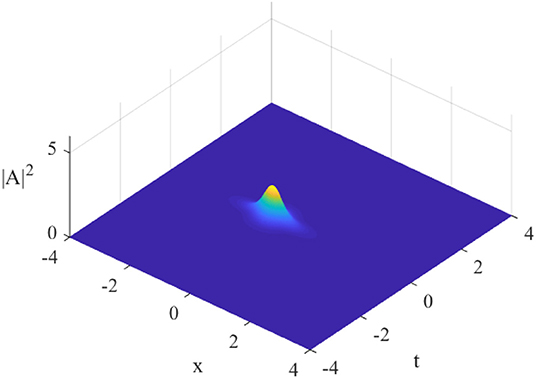
Figure 1. Wave profile of the intensity of the wave envelope in physical space, |A|² (Equation 4 through Equation 7), vs. spatial coordinate x and time t, b = 1.5. The rogue wave has one single maximum. The profile for |B|² is similar.

FIGURE 2

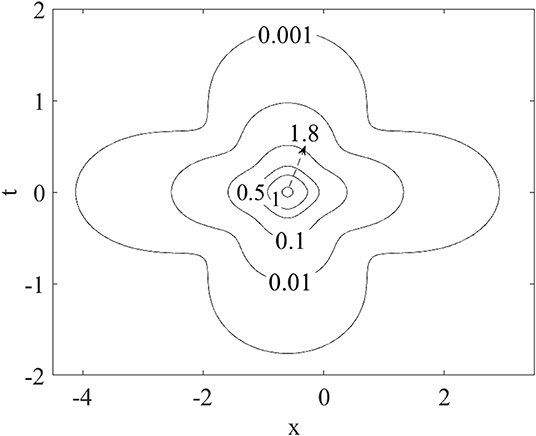
Figure 2. Planar plot of the wave intensity |A|² in physical space vs. the spatial coordinate x for one particular instant in time t, Equation (4) through Equation (7), b = 1.5. The maximum height occurs at the spatial location of x = −0.600.

3.1.2. Complex Plane

If we now consider the transverse variable x in Equation (3) as complex by analytic continuation, singularities or poles will occur when the denominator D₀₀ of Equation (4) vanishes. The numerical values can be readily found by Newton's or other standard methods. As D₀₀ is a polynomial of degree four in x for any given t, there will be four poles. For the present case of b = 1.500, a plot of the imaginary parts of the poles vs. time t is illustrated in Figure 3. At the “turning point,” where the movement of the poles (with respect to time) changes direction, the real part is again −0.600.

FIGURE 3

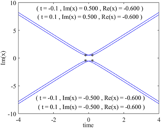
Figure 3. The trajectories of poles in the complex x plane, i.e., zeros of the denominator D₀₀ of Equation (4) to Equation (6): imaginary part of the poles vs. time t. At the turning points of the curves, the real part of the pole is −0.600, which is the spatial location of the point of maximum height in physical space.

Other than an apparently fortunate coincidence, this rather amazing match also touches a deeper theoretical question. In principle, the locations of maximum intensities (|A|², |B|²) can be determined by calculus using the expressions of Equation (4) through Equation (7). However, the present conjecture does propose another route. More precisely, we only need to select a portion of the complete analytical solution, namely, D₀₀ in the present case, and determine the location of the poles in the complex plane by extending the transverse variable by analytic continuation. On the other hand, not all points involving a change of direction of pole trajectories will automatically correspond to peaks of rogue waves. The precise necessary and sufficient conditions are still not clear. On a broader question, whether this association between maximum heights in the physical space and pole trajectories in the complex plane will hold generally for all “soliton equations” remains open. Further investigative efforts are required.

3.2. Rogue Waves With “Double Peaks”

3.2.1. Physical Space

While the rogue wave of the nonlinear Schrödinger equation always displays one single maximum for all input parameters, the present case of coherent coupling may exhibit two peaks as we increase parameter b. As an illustrative example, we select b = 3.040. The rogue wave for |A|² possesses two maxima (Figure 4). The intensity first rises to a peak, subsides slightly, and then grows to another peak before decaying into the background again. Similarly, the rogue wave for |B|² also first rises to a peak, drops to a deeper “valley,” and gains strength to attain another peak before disappearing into the background (Figure 4). Numerically, this maximum height occurs at the spatial location of x = −0.908. This whole feature can also be illustrated through planar contour plots (Figure 5).

FIGURE 4

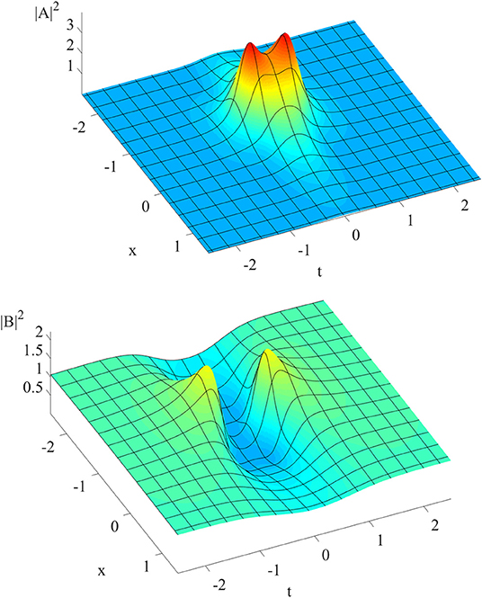
Figure 4. Wave intensities |A|² (top) and |B|² (bottom) vs. space x and time t, clearly illustrating the “double peak” structure.

FIGURE 5

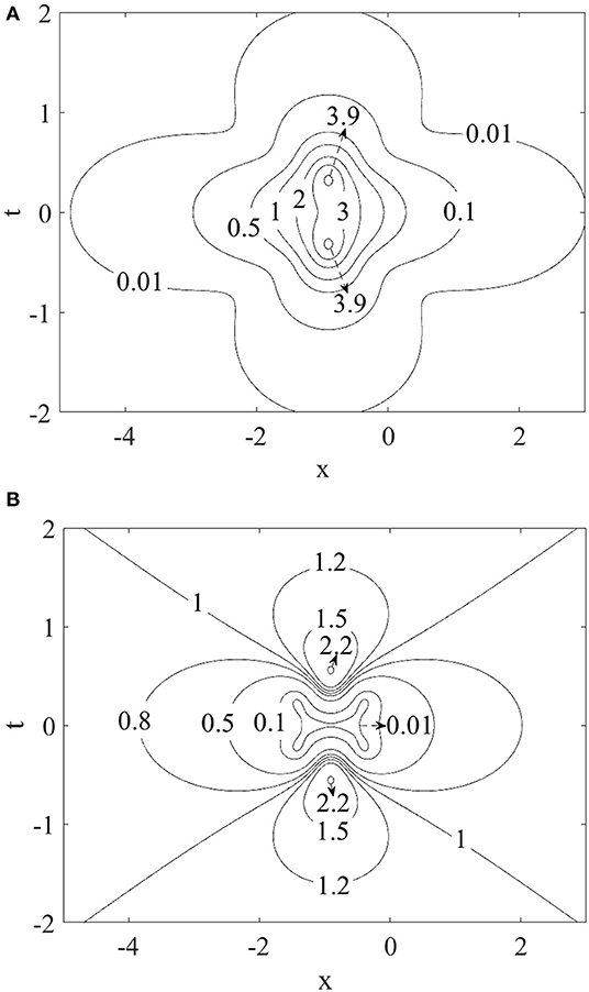
Figure 5. (A) Planar contour plot of the wave intensities |A|², illustrating the “double peak” structure. (B) Planar contour plot of the wave intensities |B|², illustrating the “double peak” structure.

3.2.2. Complex Plane

If we now allow variable x to be complex by analytic continuation, the poles arise from the zeros of D₀₀ (Equation 6). For any given time t, D₀₀ is a fourth-order polynomial, and hence there will be four pole trajectories (Figure 6). If we trace the imaginary part of the poles as a function of time, the real parts of the poles at the turning points of these trajectories attain the value of −0.908, identical to the spatial locations of maximum heights in physical space.

FIGURE 6

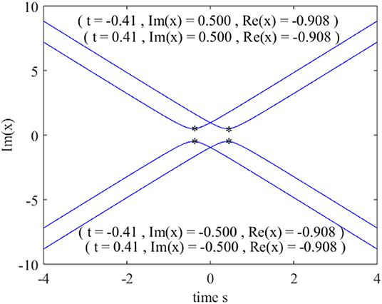
Figure 6. Pole trajectories in the complex plane by allowing the variable x to be complex by analytic continuation. Poles occur at the zeros of D₀₀ of Equation (6). The real parts of the poles at the turning points of the trajectories coincide with the locations of maximum heights of the rogue wave in physical space.

To ensure that the phenomenon just displayed is not a fortunate coincidence, we test other values of b (Table 1). The remarkable correlations between the real parts of the poles and the locations of maximum heights in physical space are again confirmed.

TABLE 1

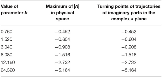
Table 1. Correlating the real parts of the poles in the complex x plane and locations of maximum heights in physical space.

From these data, we can propose an empirical, linear relation connecting the real part of the poles and parameter b (Figure 7).

FIGURE 7

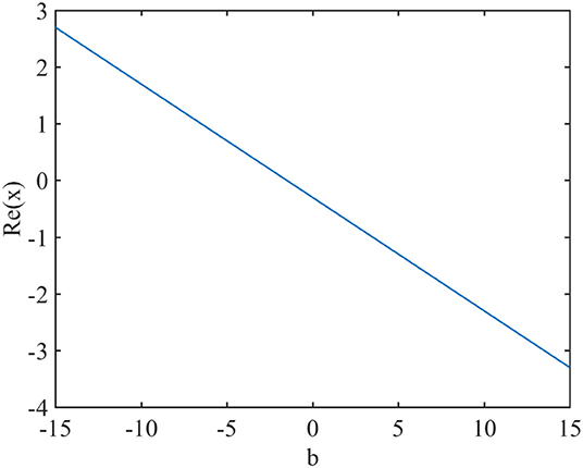
Figure 7. An empirical linear relation between the real parts of the poles at the turning points and parameter b.

4. A Schrödinger Equation With Quintic Non-Linearity

To establish further support for the conjecture outlined in Section 2, we consider a Schrödinger equation with quintic (fifth-order) nonlinearity (u = complex valued, slowly varying wave envelope):

$\begin{array}{ll}i\frac{\partial u}{\partial t}=\frac{{\partial }^{2}u}{\partial x^2}\pm ia{|u|}^2\frac{\partial u}{\partial x}\pm i\beta u^2\frac{\partial u^{*}}{\partial x}+c{|u|}^{4}u\pm d{|u|}^{2}u.& (8)\end{array}$

The parameters a, β, and d can be arbitrary, but c must be given by

$\begin{array}{ll}c=\frac{\beta (2\beta -a)}{4}& (\mathrm{9a})\end{array}$

The first- and second-order rogue waves, denoted by u₁ and u₂, respectively, can be established by Darboux transformation. One special case has been given earlier in the literature as [15]

$\begin{array}{ll}a=d=-1,\beta =1,& (\mathrm{9b})\end{array}$

$\begin{array}{ll}{u}_1=\rho {}_1^2\frac{(40t^2+4t(4x+5i)+8x^2-4ix-3)\text{ exp}(-7it/4)}{40t^2+4t(4x-3i)+8x^2-4ix+1},& (10)\end{array}$

$\begin{array}{l}{u}_2=\rho {}_2^2[(64000t^6+19200t^5(4x+5i)\\ +192t^4(360x^2+300ix-133)\\ +128t^3(272x^3+300i{x}^2-282x+375i)\\ +72t^2(192x^4+64i{x}^3-336x^2\\ +144ix-175)+12t(256x^5+64i{x}^4+64x^3\\ -288i{x}^2-468x-123i)\\ +512x^6-768i{x}^5-960x^4+384i{x}^3-792x^2\\ +180ix+45)\text{ exp}(-7it/4)]/(64000t^6\\ +19200t^5(4x-3i)+192t^4(360x^2\\ -340ix+127)+128t^3(272x^3\\ -372i{x}^2-306x-99i)+24t^2(576x^4\\ -832i{x}^3-816x^2+336ix\\ +483)+12t(256x^5-448i{x}^4-192x^3\\ -96i{x}^2+108x-75i)\\ +512x^6-768i{x}^5-192x^4-384i{x}^3\\ +360x^2-108ix+9).& (11)\end{array}$

The parameters ρ₁ and ρ₂ can be obtained from the derivations outlined in earlier references [15]. They may also be readily determined by examining the far field condition [|x|, |t| → ∞] of Equations (10) and (11), i.e., they are the roots of the algebraic equation:

$\begin{array}{l}7/4=c{({\rho }_n)}^8\pm d{({\rho }_n)}^4,n=1,2.\end{array}$

As we are concentrating on the location of the maximum height of rogue waves and the correlation with pole trajectories, we shall just consider a “normalized” height of the rogue wave u_n/(ρ_n)² (Figures 8, 9).

FIGURE 8

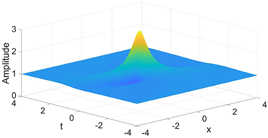
Figure 8. The amplitude of the normalized first-order rogue wave of the complex valued wave envelope u governed by a nonlinear Schrödinger equation with quintic nonlinearity, Equation (8). The profile resembles a classical Peregrine soliton.

FIGURE 9

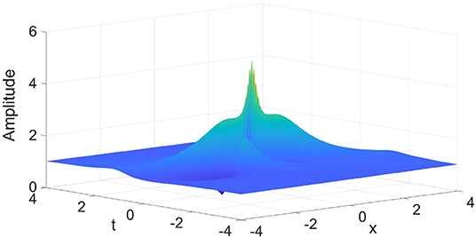
Figure 9. The amplitude of the normalized second-order rogue wave of the complex valued wave envelope u governed by a nonlinear Schrödinger equation with quintic nonlinearity, Equation (8). There is a central maximum with two smaller peaks on the sides.

The first-order rogue wave displays one single maximum and two “valleys,” resembling the properties of the well-known Peregrine soliton (Figure 8). The second-order rogue wave exhibits three peaks, one large peak in the center of the three-dimensional plot and two smaller peaks at the sides (Figure 9). These two smaller peaks are symmetrically placed and have the same amplitude but are smaller than that of the central maximum.

The locations of the points of maximum height in the physical space are again strongly correlated with the real parts of the poles in the complex plane. The matching is exact for the first-order rogue wave and the central maximum for the second-order rogue wave. For the smaller peaks on the sides, the correlation is correct up to two decimal places (Table 2).

TABLE 2

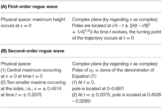
Table 2. Correlating the real parts of the poles in the complex plane and locations of maximum heights in physical space.

While this matching alone cannot predict the occurrence of rogue waves, as we need the information on the time t, nevertheless this surprising link might constitute a predictive feature on the extraordinary analytical structures these evolution equations might possess.

5. Discussions and Conclusions

The Peregrine soliton is an exact, algebraically localized solution of the nonlinear Schrödinger equation and is commonly employed as a model for rogue waves. Higher-order rational solutions also exist for this general hierarchy of evolution equations. Naturally, the algebra becomes increasingly complicated as the order increases. Schemes to locate the maxima in physical space thus become a practical necessity in addition to being of theoretical interest as the families of Schrödinger equations are widely applicable to physical sciences, e.g., fluid mechanics, optics, and plasma.

We proposed a conjecture (Section 2) which will hopefully provide an important step in this direction [8–10]. If the transverse variable of the Schrödinger equation is allowed to be complex, the real parts of the pole trajectories at the turning points will be identical to or will closely correlate with the locations of maximum heights of the rogue wave in physical space. Concurrently, this conjecture highlights deeper issues which might reveal the analytic structures of exact solutions of the family of nonlinear Schrödinger systems, as a portion of the analytic solution appears to be sufficient to give a reasonable prediction on the maximum amplitude of the wave profile.

To substantiate our earlier works [8, 10], we study further examples of Schrödinger equations here, namely, those with coherent coupling [14, 16] and quintic (fifth-order) nonlinearities [15]. The conjecture is again verified for the first and second-order rogue waves of these models.

Many challenges remain ahead. It would be fruitful to investigate other evolution systems which admit unexpectedly large displacements, e.g., rogue waves on a periodic background [17–19] and rogue waves for discrete equations [20, 21].

Data Availability Statement

The original contributions presented in the study are included in the article/supplementary material, further inquiries can be directed to the corresponding author.

Author Contributions

KWC proposed the theoretical framework. NNP performed the calculation for the case of coherent coupling, while TLC was responsible for the quintic case. All authors contributed to the article and approved the submitted version.

Funding

Partial financial support has been provided by the Research Grants Council General Research Fund contract HKU17200718.

Conflict of Interest

The authors declare that the research was conducted in the absence of any commercial or financial relationships that could be construed as a potential conflict of interest.

References

1. Peregrine DH. Water-waves, nonlinear Schrödinger-equations and their solutions. J Aust Math Soc B. (1983) 25:16–43. doi: 10.1017/S0334270000003891

CrossRef Full Text | Google Scholar

2. Craik ADD. Wave Interactions and Fluid Flows. Cambridge: Cambridge University Press (1985). doi: 10.1017/CBO9780511569548

CrossRef Full Text | Google Scholar

3. Kivshar Y, Agrawal G. Optical Solitons: From Fibers to Photonic Crystals. San Diego, CA: Academic Press (2003). doi: 10.1016/B978-012410590-4/50012-7

CrossRef Full Text | Google Scholar

4. Dysthe K, Krogstad HE, Müller P. Oceanic rogue waves. Annu Rev Fluid Mech. (2008) 40:287–310. doi: 10.1146/annurev.fluid.40.111406.102203

CrossRef Full Text | Google Scholar

5. Kharif C, Pelinovsky E, Slunyaev A. Rogue Waves in the Ocean. Berlin: Springer (2009).

Google Scholar

6. Onorato M, Residori S, Bortolozzo U, Montina A, Arecchi FT. Rogue waves and their generating mechanisms in different physical contexts. Phys Rep. (2013) 528:47–89. doi: 10.1016/j.physrep.2013.03.001

CrossRef Full Text | Google Scholar

7. Chen SH, Baronio F, Soto-Crespo JM, Grelu P, Mihalache D. Versatile rogue waves in scalar, vector, and multidimensional nonlinear systems. J Phys A Math Theor. (2017) 50:463001. doi: 10.1088/1751-8121/aa8f00

CrossRef Full Text | Google Scholar

8. Chung WC, Chiu TL, Chow KW. Employing the dynamics of poles in the complex plane to describe properties of rogue waves: case studies using the Boussinesq and complex modified Korteweg–de Vries equations. Nonlinear Dyn. (2020) 99:2961–70. doi: 10.1007/s11071-020-05475-z

CrossRef Full Text | Google Scholar

9. Chiu TL, Liu TY, Chan HN, Chow KW. The dynamics and evolution of poles and rogue waves for nonlinear Schrödinger equations. Commun Theor Phys. (2017) 68:290–4. doi: 10.1088/0253-6102/68/3/290

CrossRef Full Text | Google Scholar

10. Liu TY, Chiu TL, Clarkson PA, Chow KW. A connection between the maximum displacements of rogue waves and the dynamics of poles in the complex plane. Chaos. (2017) 27:091103. doi: 10.1063/1.5001007

PubMed Abstract | CrossRef Full Text | Google Scholar

11. Konno K, Ito H. Nonlinear interactions between solitons in complex t-plane 1. J Phys Soc Jpn. (1987) 56:897–904. doi: 10.1143/JPSJ.56.897

CrossRef Full Text | Google Scholar

12. Konno K. Nonlinear interactions between solitons in complex t-plane 2. J Phys Soc Jpn. (1987) 56:1334–9. doi: 10.1143/JPSJ.56.1334

CrossRef Full Text | Google Scholar

13. Ankiewicz A, Clarkson PA, Akhmediev N. Rogue waves, rational solutions, the patterns of their zeros and integral relations. J Phys A Math Theor. (2010) 43:122002. doi: 10.1088/1751-8113/43/12/122002

CrossRef Full Text | Google Scholar

14. Sun WR, Tian B, Jiang Y, Zhen HL. Optical rogue waves associated with the negative coherent coupling in an isotropic medium. Phys Rev E. (2015) 91:023205. doi: 10.1103/PhysRevE.91.023205

PubMed Abstract | CrossRef Full Text | Google Scholar

15. Wang L, Jiang DY, Qi FH, Shi YY, Zhao YC. Dynamics of the higher-order rogue waves for a generalized mixed nonlinear Schrödinger model. Commun Nonlinear Sci Numer Simulat. (2017) 42:502–19. doi: 10.1016/j.cnsns.2016.06.011

CrossRef Full Text | Google Scholar

16. Zhang CR, Tian B, Liu L, Chai HP, Du Z. Vector breathers with the negatively coherent coupling in a weakly birefringent fiber. Wave Motion. (2019) 84:68–80. doi: 10.1016/j.wavemoti.2018.09.003

CrossRef Full Text | Google Scholar

17. Peng WQ, Tian SF, Wang XB, Zhang TT. Characteristics of rogue waves on a periodic background for the Hirota equation. Wave Motion. (2020) 93:102454. doi: 10.1016/j.wavemoti.2019.102454

CrossRef Full Text | Google Scholar

18. Li M, Fu HM, Wu CF. General soliton and (semi-)rational solutions to the nonlocal Mel'nikov equation on the periodic background. Stud Appl Math. (2020) 145:97–136. doi: 10.1111/sapm.12313

CrossRef Full Text | Google Scholar

19. Chen JB, Pelinovsky DE, White RE. Rogue waves on the double-periodic background in the focusing nonlinear Schrödinger equation. Phys Rev E. (2019) 100:052219. doi: 10.1103/PhysRevE.100.052219

PubMed Abstract | CrossRef Full Text | Google Scholar

20. Ortiz AK, Prinari B. Inverse scattering transform for the defocusing Ablowitz-Ladik system with arbitrarily large nonzero background. Stud Appl Math. (2019) 143:373–403. doi: 10.1111/sapm.12282

CrossRef Full Text | Google Scholar

21. Wang HT, Wen XY. Soliton elastic interactions and dynamical analysis of a reduced integrable nonlinear Schrödinger system on a triangular-lattice ribbon. Nonlinear Dyn. (2020) 100:1571–87. doi: 10.1007/s11071-020-05587-6

CrossRef Full Text | Google Scholar