Thermodynamic Properties of the Parabolic-Well Fluid

1 Introduction

The issue of Frontiers in Physics this paper belongs to is devoted to commemorating the celebration of fifty consecutive annual Winter Meetings in Statistical Physics in Mexico. Therefore, we have chosen to write on a subject that has been present in these meetings from the beginning; namely, the thermodynamic properties of fluids that we are persuaded can still offer some interesting results.

We begin by recalling that, in an attempt to prove the validity of the thermodynamic limit of classical statistical mechanics, van Hove [1] introduced in 1949 a potential $\varphi \left(r\right)$ consisting of a hard core of radius $r_0$ and a finite-range attractive tail. The actual form of this so-called van Hove potential is

$\varphi \left(r\right)=\{\begin{array}{cc}\infty ,& 0\le r\le r_0,\\ <0,& r_0<r\le b\\ >-{\epsilon }_0,& r_0<r\le b,\\ 0,& r>b,\end{array}(1)$

where r is the distance, b corresponds to the range, and $-{\epsilon }_0$ corresponds to the lower bound of the attractive tail, whose form is rather arbitrary. It should be pointed out that two popular models of intermolecular potentials used in liquid state physics, namely, the triangle-well potential and the square-well potential, fulfill the condition of being van Hove potentials and their thermodynamic properties have been thoroughly studied (see, for instance, Refs. [2–11] for the former model and Refs. [12–24] for the latter and references therein). Surprisingly, as far as we know, the parabolic-well potential, which is also a van Hove potential, has not been used for that purpose. The main aim of this paper is to contribute to partly remedying this situation.

We consider a parabolic-well fluid whose molecules interact with a potential of the form

$u\left(x\right)=\{\begin{array}{cc}\infty ,& 0\le x\le 1,\\ \epsilon \left[{\left(\frac{x-1}{\lambda -1}\right)}^2-1\right],& 1<x\le \lambda ,\\ 0,& x>\lambda ,\end{array}(2)$

where $x=r/\sigma$ is the reduced distance (r being the distance), σ is the diameter of the hard core, $\epsilon >0$ is the well depth, and $\lambda >1$ is the potential range. As it occurs with other relatively simple models, the main asset of this model potential is probably that, despite being an idealized representation, it nevertheless contains the main features of true molecular interactions in fluids, namely, a repulsive hard-core and an attractive interaction that continuously goes to zero as the intermolecular distance increases. In this regard, it is interesting to recall what Widom [25] pointed out in the case of the square-well fluid: “Where I speak of the necessity to treat accurately the effects of the attractive or repulsive forces, I do not mean that it is important to know the corresponding part of $\varphi \left(r\right)$ with quantitative accuracy. Indeed, even if the $\varphi \left(r\right)$ of Figure 1 were idealized as a square-well potential, as in Figure 3, but the statistical mechanical consequences of such a potential were then determined without further approximation, there would undoubtedly result in an essentially correct description of all the macroscopic properties of matter throughout a vast region of the p and T plane, including the neighborhoods of the triple and critical points. Thus, what matters is not the quantitative accuracy of the assumed $\varphi \left(r\right)$, but rather the qualitative accuracy of the resulting spatial correlations of molecular positions; the triple and critical points are distinguished by having the relevant qualitative features of this correlation, and the nature of its propagation through the fluid, determined primarily by the short-range repulsive forces between molecules, or by the longer ranged attractive forces, respectively.” Something similar may be said about the parabolic-well potential. In fact, an interesting asset of this model is that its thermodynamic properties are readily amenable for treatment within the second-order thermodynamic perturbation theory of Barker and Henderson [26]. Within this approach, in order to derive the Helmholtz free energy of the parabolic-well fluid, two ingredients are required: on the one hand, one needs the Helmholtz free energy of the reference hard-sphere fluid of diameter σ. On the other hand, one also requires an expression for the radial distribution function $g_{HS}\left(x\right)$ of the hard-sphere fluid. In this work, we will profit from the availability of a method [27], the so-called rational function approximation (RFA) method, to (analytically) obtain an approximate $g_{HS}\left(x\right)$ which is thermodynamically consistent with the equation of state of the hard-sphere fluid and make use of this fact to derive the equation of state of the parabolic-well fluid.

FIGURE 1

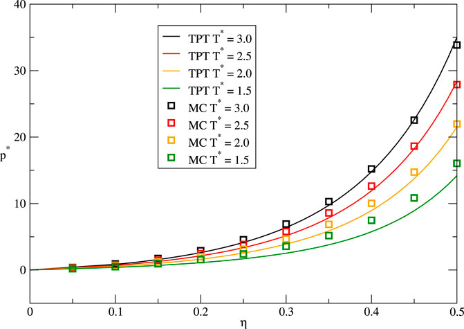
FIGURE 1. Various isotherms of the parabolic-well fluid for $\lambda =1.25$. The label TPT indicates that the results have been obtained using thermodynamic perturbation theory while the label MC refers to Monte Carlo simulation results.

The paper is organized as follows. In the next section, we recall the main aspects of the RFA method for the computation of $g_{HS}\left(x\right)$ and provide the explicit expression for this quantity in the first coordination shell. This is followed in Section 3 with the completely analytic derivation of the equation of state of the parabolic-well fluid within the second-order Barker-Henderson thermodynamic perturbation theory in the macroscopic compressibility approximation and taking the hard-sphere fluid as the reference system. Section 4 contains some illustrative results for the reduced pressure of the parabolic-well fluid and a comparison with our own Monte Carlo and Event-driven Molecular Dynamics simulation data. We close the paper in the final section with further discussion and some concluding remarks.

2 The Rfa Method For The Computation of The Radial Distribution Function of The Hard-Sphere Fluid

In this section, we provide the analytic result for the radial distribution function (rdf) of the hard-sphere fluid $g_{HS}\left(x\right)$, as derived with the RFA method [27], and its explicit expression in the range $1<x\le 2$. We begin by recalling two important relationships between the thermodynamic and structural properties of the hard-sphere fluid derived from statistical mechanics. On the one hand, the compressibility factor $Z_{HS}=\frac{p}{\rho k_{B}T}$ (where p is the pressure, ρ the number density, $k_B$ the Boltzmann constant, and T the absolute temperature) of the hard-sphere fluid is related to the contact value of the rdf $g_{HS}\left(1^{+}\right)$ through

$Z_{HS}=1+4\eta g_{HS}\left(1^{+}\right),(3)$

where $\eta =\pi \rho {\sigma }^3/6$ is the packing fraction. On the other hand, the hard-sphere isothermal susceptibility ${\chi }_{HS}\equiv {\left[\frac{d\left(\eta Z_{HS}\left(\eta \right)\right)}{d\eta }\right]}^{-1}$ is related to the rdf through

${\chi }_{HS}=1+24\eta {\displaystyle {\int }_0^{\infty }dx}{x}^2\left[g_{HS}\left(x\right)-1\right].(4)$

In the RFA method [27], the Laplace transform of $x{g}_{HS}\left(x\right)$ is taken to be given by

$G\left(t\right)=\mathrm{ℒ}\left\{x{g}_{HS}\left(x\right)\right\}=\frac{t}{12\eta }\frac{1}{1-e^t\Phi \left(t\right)},(5)$

where

$\Phi \left(t\right)=\left(1+S_{1}t+S_2{t}^2+S_3{t}^3+S_4{t}^4\right)/\left(1+L_{1}t+L_2{t}^2\right),$

and the six coefficients $S_1$, $S_2$, $S_3$, $S_4$, $L_1$, and $L_2$ (which depend on the packing fraction) may be evaluated in an algebraic form by imposing the following requirements: (i) ${\chi }_{HS}$ must be finite and hence the first two integral moments of the total correlation function $h\left(x\right)\equiv g\left(x\right)-1$, i.e., ${\displaystyle {\int }_0^{\infty }dx}{x}^{n}h\left(r\right)$ with $n=\mathrm{1,2}$, must be well defined; (ii) the approximation must be thermodynamically consistent with a prescribed equation of state; i.e., the thermodynamic relationship ${\chi }_{HS}={\left[\frac{d\eta Z_{HS}\left(\eta \right)}{d\eta }\right]}^{-1}$ must be satisfied. Using the first requirement, one finds that $L_1$, $S_1$, $S_2$, and $S_3$ are linear functions of $L_2$ and $S_4$. Imposing the requirement (ii) leads to explicit expressions for $L_2$ and $S_4$ in terms of ${\chi }_{HS}$ and $Z_{HS}$ [27]. Finally, the expressions for all the coefficients are as follows:

$L_1=\frac{1}{2}\frac{\eta +12\eta L_2+2-24\eta S_4}{2\eta +1},(6)$

$S_1=\frac{3}{2}\eta \frac{-1+4L_2-8S_4}{2\eta +1},(7)$

$S_2=-\frac{1}{2}\frac{-\eta +8\eta L_2+1-2L_2-24\eta S_4}{2\eta +1},(8)$

$S_3=\frac{1}{12}\frac{2\eta -{\eta }^2+12{\eta }^2{L}_2-12\eta L_2-1-72{\eta }^2{S}_4}{\left(2\eta +1\right)\eta },(9)$

$L_2=-3\left(Z_{HS}-1\right)S_4,(10)$

$S_4=\frac{1-\eta }{36\eta \left(Z_{HS}-1/3\right)}{[1-\left[1+\frac{Z_{HS}-1/3}{Z_{HS}-Z_{PY}}\left(\frac{{\chi }_{HS}}{{\chi }_{PY}}-1\right)\right]]}^{1/2}.(11)$

Here, $Z_{PY}=\frac{1+2\eta +3{\eta }^2}{{\left(1-\eta \right)}^2}$ and ${\chi }_{PY}=\frac{{\left(1-\eta \right)}^4}{{\left(1+2\eta \right)}^2}$ are the compressibility factor and isothermal susceptibility arising in the Percus-Yevick theory. To close the problem, one has to give an expression for $Z_{HS}$, so all the procedure is a function of this choice. For a given $Z_{HS}$, the radial distribution function is given by

$g_{HS}\left(x\right)=\{\begin{array}{cc}0,& 0\le x<1,\\ \frac{1}{12\eta x}{\displaystyle \sum _{n=1}^{\infty }{\phi }_n\left(x-n\right)\theta \left(x-n\right)},& x\ge 1\end{array}(12)$

with $\theta \left(x-n\right)$ being the Heaviside step function and

${\phi }_n\left(x\right)={\mathrm{ℒ}}^{-1}\left\{-t{\left[\Phi \left(t\right)\right]}^{-n}\right\}.(13)$

Explicitly, using the residues theorem,

${\phi }_n\left(x\right)=-{\displaystyle \sum _{n=1}^4{e}^{t_{i}x}}{\displaystyle \sum _{m=1}^n\frac{A_{mn}\left(t_i\right)}{\left(n-m\right)!}{x}^{n-m},}(14)$

where

$A_{mn}\left(t_i\right)=\underset{t\to t_i}{\lim }\frac{1}{\left(m-1\right)!}{\left(\frac{d}{dt}\right)}^{m-1}\left(t-t_i\right)t{\left[\Phi \left(t\right)\right]}^{-n},(15)$

with $t_i$ being the four roots of $1+S_{1}t+S_2{t}^2+S_3{t}^3+S_4{t}^4=0$; namely,

$t_1=-\frac{S_3}{4S_4}+y_p-y_n,(16)$

$t_2=-\frac{S_3}{4S_4}+y_p+y_n,(17)$

$t_3=-\frac{S_3}{4S_4}-y_p-y_m,(18)$

$t_4=-\frac{S_3}{4S_4}-y_p+y_m,(19)$

where

$y_p=-\frac{1}{2}\sqrt{\frac{S_3^2}{4S_4^2}-\frac{2S_2}{3S_4}+y_r+\frac{y_s}{3S_4}},(21)$

$y_r=-\frac{S_2^2-3S_1{S}_3+12S_4}{3S4y_s},(22)$

$y_n=\frac{1}{2}\sqrt{\frac{S_3^2}{4S_4^2}-\frac{4S_2}{3S_4}-y_r-\frac{y_s}{3S_4}-\frac{S_3^3}{8y_p{S}_4^3}+\frac{S_2{S}_3}{2y_p{S}_4^2}-\frac{S_1}{y_p{S}_4}},(23)$

$y_m=\frac{1}{2}\sqrt{\frac{S_3^2}{4S_4^2}-\frac{4S_2}{3S_4}-y_r-\frac{y_s}{3S_4}+\frac{S_3^3}{8y_p{S}_4^3}-\frac{S_2{S}_3}{2y_p{S}_4^2}+\frac{S_1}{y_p{S}_4}},(24)$

$y_s=-\frac{1}{2^{1/3}}{\left[y_t+\sqrt{-4{\left(S_2^2-3S_1{S}_3+12S_4\right)}^3+y_t^2}\right]}^{1/3},(25)$

$y_t=2S_2^3+9S_1{S}_2{S}_3+27S_3^2+27S_1^2{S}_4-72S_2{S}_4.(26)$

As we will indicate below, once $Z_{HS}\left(\eta \right)$ has been chosen, Eqs. 5–26 are all that is needed to evaluate the first- and second-order perturbation terms for the free energy of the parabolic-well fluid within the Barker-Henderson thermodynamic perturbation theory taking the hard-sphere fluid as the reference system. To close this section and for later use, we now write the explicit expression for the radial distribution function up to the first coordination shell which reads

$g_{HS}\left(x\right)=\{\begin{array}{cc}0,& 0\le x<1,\\ {\displaystyle \sum _{i=1}^4\frac{a_i}{x}{e}^{t_i\left(x-1\right)}},& 1\le x\le 2\end{array}(27)$

where

$a_i=\frac{-t_i\left(1+L_1{t}_i+L_2{t}_i^2\right)}{12\eta \left(S_1+2S_2{t}_i+3S_3{t}_i^2+4S_4{t}_i^3\right)}\left(i=\mathrm{1,2,3,4}\right).(28)$

3 Thermodynamic Perturbation Theory and the Equation of State of the Parabolic-Well Fluid

Perturbation approaches for the computation of thermodynamic properties of fluids are well established theoretical tools [28, 29]. In the Barker-Henderson perturbation theory [26], one splits the potential into a hard-sphere part and a perturbation part; namely, $u\left(r\right)=u_{HS}\left(r\right)+u_1\left(r\right)$, where

$u_{HS}\left(x\right)=\{\begin{array}{cc}\infty ,& 0\le x\le 1,\\ 0,& x>1\end{array}(29)$

and

$u_1\left(x\right)=\{\begin{array}{cc}0,& 0\le x\le 1,\\ \epsilon \left[{\left(\frac{x-1}{\lambda -1}\right)}^2-1\right],& 1<x\le \lambda ,\\ 0,& x>\lambda \end{array}(30)$

Once this separation has been made, the Helmholtz free energy per particle of the parabolic-well fluid is expressed as a power series in the inverse of the reduced temperature $T^{\ast }=k_{B}T/\epsilon$, which up to second order reads

$\frac{f}{N{k}_{B}T}=\frac{f_{HS}}{N{k}_{B}T}+\frac{1}{T^{\ast }}\frac{f_1}{N{k}_{B}T}+\frac{1}{T^{\ast 2}}\frac{f_2}{N{k}_{B}T}(31)$

Here, N is the number of particles and $f_{HS}$ stands for the Helmholtz free energy of the reference hard-sphere fluid while $f_1$ and $f_2$ (this latter in the so-called macroscopic compressibility approximation) are given, respectively, by

$\frac{f_1}{N{k}_{B}T}=\frac{12\eta }{\epsilon }{\displaystyle {\int }_1^{\lambda }{g}_{HS}\left(x\right)u_1\left(x\right)x^{2}dx}(32)$

and

$\frac{f_2}{N{k}_{B}T}=\frac{6\eta {\chi }_{HS}}{{\epsilon }^2}{\displaystyle {\int }_1^{\lambda }{g}_{HS}\left(x\right)u_1^2\left(x\right)x^{2}dx}.(33)$

Note that we have made use of the fact that $g_{HS}\left(x\right)$ vanishes for $0\le x<1$ and of the expression for $u_1\left(x\right)$ given in Eq. 30, respectively, to set the lower and upper limits of the integrals in Eqs. 32, 33. In turn, the equation of state of the parabolic-well fluid in this approximation is given by

$Z\equiv \frac{p}{\rho k_{B}T}=Z_{HS}+\frac{1}{T^{\ast }}\eta \frac{\partial }{\partial \eta }\left(\frac{f_1}{N{k}_{B}T}\right)+\frac{1}{T^{\ast 2}}\eta \frac{\partial }{\partial \eta }\left(\frac{f_2}{N{k}_{B}T}\right).(34)$

And, the chemical potential may be readily obtained as

$\frac{\mu }{k_{B}T}=\frac{f}{N{k}_{B}T}+Z,(35)$

where $\frac{f}{N{k}_{B}T}$ is given in Eq. 31, together with Eqs. 32, 33, and Z is given in Eq. 34. So, provided we choose $Z_{HS}$, which of course also determines ${\chi }_{HS}$ and $f_{HS}$, and take $g_{HS}$ to be the one computed with the RFA approach and such compressibility factor, the completely analytic formulation of the second-order Barker-Henderson thermodynamic perturbation theory in the macroscopic compressibility approximation for the parabolic-well fluid taking the hard-sphere fluid as the reference system has been derived. In our subsequent calculations, we will be restricted to relatively narrow wells ($1<\lambda \le 2$) so that Eq. 27 for $g_{HS}\left(r\right)$ will be used. Furthermore, $Z_{HS}$ and ${\chi }_{HS}$ will be chosen to be those corresponding to the Carnahan-Starling (CS) equation of state [30]; namely,

$Z_{HS}\left(\eta \right)\equiv Z_{CS}\left(\eta \right)=\frac{1+\eta +{\eta }^2-{\eta }^3}{{\left(1-\eta \right)}^3}(36)$

and

${\chi }_{HS}\left(\eta \right)\equiv {\chi }_{CS}\left(\eta \right)=\frac{{\left(1-\eta \right)}^4}{1+4\eta +4{\eta }^2-4{\eta }^3+{\eta }^4}.(37)$

Further, from the CS equation of state, it also follows that

$\frac{f_{HS}\left(\eta \right)}{N{k}_{B}T}=\frac{f_{CS}\left(\eta \right)}{N{k}_{B}T}=-1+\ln \frac{6\eta }{\pi }+\frac{\left(4-3\eta \right)\eta }{{\left(1-\eta \right)}^2}.(38)$

The availability of the completely analytic (albeit approximate) forms of the Helmholtz free energy and the equation of state of the system (which are themselves not very illuminating and therefore will not be explicitly written down [31]) allows us in principle to compute, for a given value of λ, the compressibility factor using Eq. 34, the vapor-liquid coexistence curve from the equality of pressures, and chemical potentials of the two phases and also to obtain the critical point in the usual way.

Preliminary results for the isotherms will be presented in the following section, together with a comparison with our simulation data. But before presenting such results, we will take advantage of the simple form of the intermolecular potential of this fluid to compute its second virial coefficient. This is given by

$B_2\left(T\right)\equiv -2\pi {\sigma }^3{\displaystyle {\int }_0^{\infty }{x}^2\left(e^{\frac{u\left(x\right)}{k_{B}T}}-1\right)dx}(39)$

$=-\frac{\pi }{6}{\sigma }^3[\frac{6k_{B}T}{\epsilon }\left(1-2e^{\frac{\epsilon }{k_{B}T}}+\lambda \right){\left(\lambda -1\right)}^2-4{\lambda }^3$

$+3\frac{\sqrt{\pi k_{B}T}{e}^{\frac{\epsilon }{k_{B}T}}}{{\epsilon }^{3/2}}\left(2\epsilon +k_{B}T{\left(\lambda -1\right)}^2\right)\left(\lambda -1\right)Erf\left(\sqrt{\frac{\epsilon }{k_{B}T}}\right)].$

Equation 39, which to the best of our knowledge has not been reported before, allows us to obtain the Boyle temperature $T_B$ of the parabolic-well fluid as a function of λ by equating $B_2\left(T_B\right)$ to zero and solving numerically for $T_B$. In Table 1, we show some particular values and, for comparison, we also include the values corresponding to triangle-well and square-well fluids with the same range λ.

TABLE 1

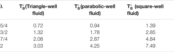
TABLE 1. Reduced Boyle temperatures $T_B^{\ast }\equiv k_B{T}_B/\epsilon$ (up to three significant figures) of triangle-well, parabolic-well, and square-well fluids for various values of the range λ.

To close this section, we will also take advantage of the knowledge of the second virial coefficient, to obtain estimates of the critical temperature according to the Vliegenthart and Lekkerkerker criterion [32], namely, from equating this coefficient with $-6v_m$, where $v_m=\frac{\pi }{6}{\sigma }^3$ is the volume of the spherical core. The results for given values of the range are given in Table 2, where we have also included such estimates for the cases of the triangle-well and square-well fluids with the same range λ.

TABLE 2

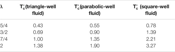
TABLE 2. Estimates of the reduced critical temperatures $T_c^{\ast }\equiv k_B{T}_c/\epsilon$ (up to three significant figures) of triangle-well, parabolic-well, and square-well fluids for various values of the range λ, as obtained from the second virial coefficient and the use of the Vliegenthart and Lekkerkerker criterion.

Note that, for all three model fluids, the values of both the reduced Boyle temperatures and the estimates of the reduced critical temperatures increase as the range λ is increased. Also note that the geometrical form of the well influences such values as reflected in the fact that, for the same value of the range, the ones corresponding to the triangle-well fluid are smaller than those of the parabolic-well fluid which, in turn, are smaller than those of the square-well fluid.

4 Illustrative Results

Now we return to our main aim. In order to assess the value of the thermodynamic perturbation theory approach presented in the previous section, we have carried out NVT Monte Carlo (MC) simulations to compute the pressure of parabolic-well fluids for various values of the range $\lambda \le 2$ and supercritical temperatures for later comparison with our theoretical results. The details of such simulations are as follows. The number of particles in our simulations is $N=1372$ and we have considered a cubic box, of length L and with periodic boundary conditions. Reduced units are used, so that lengths are expressed in units of σ ($L=l\sigma$, with l a pure number), the reduced temperature is $T^{\ast }$, the packing fraction is $\eta =\frac{\pi }{6}\frac{N}{V}{\sigma }^3$ (where $V=L^3$ is the volume), and the reduced pressure is $p^{\ast }=p{\sigma }^3{\epsilon }^{-1}$.

For the sake of illustration, we report here the results of the simulations for $\lambda =1.25$ and 1.75, along various isotherms. For each isotherm, eight different packing fraction values $\eta =0.05$ to 0.5 with $\Delta \eta =0.05$ were simulated in order to compute the reduced pressure $p^{\ast }$. Each run was carried out using $1.5\cdot {10}^6$ Monte Carlo steps (MCS) discarding the first ${10}^6$ MCS for equilibration, and the properties were measured every 20 MCS and averaged every 1000 MCS; furthermore, for each packing fraction, the values of $p^{\ast }$ were averaged over 20 parallel simulations to obtain better statistics.

Finally, the pressure was calculated using the expression

$p^{\ast }=\frac{6}{\pi }\eta T^{\ast }\left[1+4\eta g_{PW}\left(1^{+}\right)-\frac{4\eta }{T^{\ast }}{\displaystyle {\int }_1^{\lambda }{g}_{PW}\left(x\right)\frac{d{u}_1^{\ast }\left(x\right)}{dx}{x}^{3}dx}\right].(40)$

Here, $u_1^{\ast }\left(x\right)=u_1\left(x\right)/\epsilon$, $g_{PW}\left(x\right)$ is the radial distribution function of the parabolic-well fluid (computed in the usual way [33] with the subscript PW standing for parabolic well), and the second term on the right-hand side of Eq. 40, obtained following a similar procedure to the one used by Rotenberg [12] in the case of the square-well fluid, accounts for the hard-core contribution to the parabolic-well potential.

In Figures 1‐3, we show the comparison between the results of the isotherms obtained with the thermodynamic perturbation theory and from simulation. Note the good agreement between theoretical and simulation results for all the values of $T^{\ast }$ above the critical temperature that we considered.

On the other hand, the subcritical isotherms were obtained by means of Molecular Dynamics (MD) Event-driven simulations. We have performed event-driven simulations of $N=108000$ elastic smooth spheres carried out with the DynamO software package [34]. The spheres interact by a stepped parabolic-well type potential [35–37], a discretized version consisting of a sequence of 15 steps of widths $0.05\sigma$, steps more than reasonable in most instances [37]. We have used σ, $\tau =\sqrt{m{\sigma }^2/\epsilon }$, m, and $T^{\ast }$ as units of length, time, mass, and temperature, respectively. The MD event-driven simulations were performed for one value of the range of the potential, namely, $\lambda =1.75$, along the isotherms $T^{\ast }=1.1,1.0$ and 0.7. In the first stage, we have performed NVT simulations with an Andersen thermostat during $2\times {10}^8$ collisions, and after the equilibration, the second stage of NVE simulations with a duration of $8\times {10}^8$ collisions was performed [38]. The full pressure tensor for the system was determined by means of the expression

$P=P_{kinetic}+P_{\mathit{int}eraction}(41)$

where the kinetic pressure is given by

$P_{kinetic}=\frac{1}{2V}{\displaystyle \sum _i^N{v}_i{v}_i,}(42)$

with $v_i{v}_i$ being a dyadic product which yields a matrix result and the masses of the particles are set as $m_i=1$. The contribution to the pressure due to interactions is given by

$P_{\mathit{interaction}}=\frac{1}{V{t}_{sim}}{\displaystyle \sum _{ij}^{event}\Delta p_i{r}_{ij},}(43)$

where the summation is over each two-particle $i,j$ event interaction, $t_{sim}$ is the total simulation time, $\Delta p_i$ is the momentum impulse on particle i, and $r_{ij}=r_i-r_j$ is the separation vector between the interacting particles. Finally, the hydrostatic pressure, which in this instance coincides with the reduced pressure, was computed from the trace of the tensor

$p^{\ast }=tr\left(P\right)/3=\left(P_{xx}+P_{yy}+P_{zz}\right)/3.(44)$

In Figure 2, we show the comparison of the subcritical isotherms obtained with the thermodynamic perturbation theory and from simulation for a range $\lambda =1.75$. The typical van der Waals loop is clearly seen for the theoretical isotherm with $T^{\ast }=0.7$ (which grossly underestimates the simulation data) and is still present in the isotherms with $T^{\ast }=1$ and $T^{\ast }=1.1$, respectively. On the other hand, we have checked both through Monte Carlo and Event-driven MD simulations and also through the outcome of the thermodynamic perturbation theory that the isotherm with $T^{\ast }=1.35$ (not shown), which according to the Vliegenthart and Lekkerkerker criterion should be the critical one, is a supercritical isotherm. In fact, the simulation data indicate that the real critical isotherm for this value of the range lies above but close to the one corresponding to the theoretical curve for $T^{\ast }=1.1$.

FIGURE 2

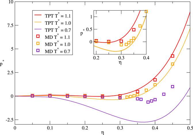
FIGURE 2. Various subcritical isotherms of the parabolic-well fluid for $\lambda =1.75$. The label TPT indicates that the results have been obtained using thermodynamic perturbation theory while the label MD refers to Event-driven Molecular Dynamics simulation results. The inset shows an enlargement of the intermediate packing fraction region for the isotherms with $T^{\ast }=1.0$ and $T^{\ast }=1.1$.

While it is clear from Figures 1–3 that the qualitative trends observed in all the simulation results are correctly accounted for by the theory, a better perspective of its performance may be gained by looking at the quantitative differences. Therefore, in Table 3, we display the actual numerical values for a couple of isotherms. In both cases, it is clear that the good qualitative agreement seen in Figures 1, 2, respectively, is not accompanied by quantitative agreement. In fact, the first theoretical isotherm ($\lambda =1.25$ and $T^{\ast }=1.5$), which is a supercritical isotherm, yields an underestimation of the reduced pressure when compared to the simulation values. On the other hand, for the second isotherm ($\lambda =1.75$ and $T^{\ast }=1.1$), which is subcritical, the general overall trend is that the theoretical curve overestimates the value of the reduced pressure. As one would expect, in the case of the supercritical isotherms, the quantitative agreement is improved as the reduced temperature is increased.

FIGURE 3

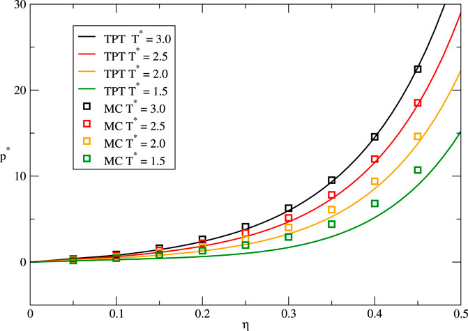
FIGURE 3. Various isotherms of the parabolic-well fluid for $\lambda =1.75$. The label TPT indicates that the results have been obtained using thermodynamic perturbation theory while the label MC refers to Monte Carlo simulation results.

TABLE 3

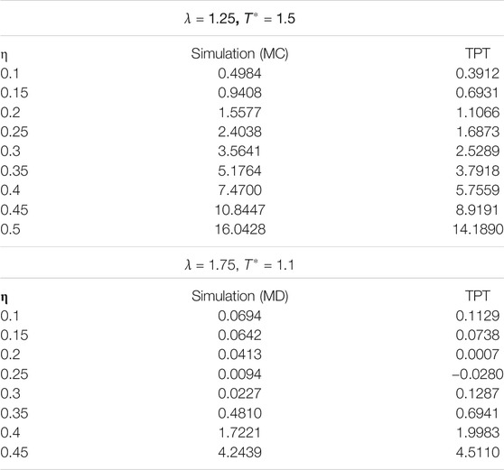
TABLE 3. Theoretical and simulation results for the reduced pressure at various packing fractions in two isotherms of the parabolic-well fluid. The labels MC, MD, and TPT stand for Monte Carlo, Event-driven MD, and thermodynamic perturbation theory, respectively.

5 Concluding Remarks

In this paper, we have addressed the study of the thermodynamic properties of a fluid whose molecules interact through a parabolic-well potential. For this model, we obtained the exact second virial coefficient which in turn allowed us to compute the Boyle temperature and to estimate the critical temperature for arbitrary values of the potential range λ. The parabolic-well potential is in the same family as the triangle-well potential and the square-well potential, being in some sense intermediate between the other two. A reflection of this is the behavior of both the Boyle temperatures and the estimates of the critical temperatures in which, for a fixed range, the values corresponding to the parabolic-well potential lie between the ones corresponding to the other two. Whether this points out to a deeper relationship between the geometrical shape of the well and the location of the critical point in van Hove fluids is not clear to us at this stage but might be worth considering in the future.

In order to obtain further analytic results, we considered a thermodynamic perturbation theory approach for this fluid within the Barker-Henderson second-order macroscopic compressibility approximation and taking the hard-sphere fluid as the reference fluid. Restricting ourselves to values of the range in the interval $1<\lambda \le 2$ and evaluating the radial distribution function of the hard-sphere fluid according to the RFA method with the CS equation of state, we were able to derive (albeit approximate) fully analytic expressions for the Helmholtz free energy, the equation of state, and the chemical potential of the parabolic-well fluid. With such expressions, we were able to compute theoretically various isotherms for a given potential range. These were subsequently compared to our own Monte Carlo NVT and Event-driven MD simulation results. It must be emphasized that these simulation data are to our knowledge the only ones available in the literature for this system.

It should be clear that the calculations that we have presented in the previous section are still preliminary but we want to stress that further work on this subject is currently being carried out. Nevertheless, at this stage, a few additional comments are in order. We begin by pointing out that the qualitative agreement between the results for the isotherms above the critical one obtained from thermodynamic perturbation theory and those stemming out of NVT Monte Carlo simulations, as well as the improvement of the quantitative agreement as the reduced temperature is increased, although clearly rewarding, are not very surprising in view of the fact that our theoretical approximation relies on the convergence of the perturbation expansion for high temperatures. Also rewarding is the fact that the results of the Event-driven MD simulation for the isotherm $T^{\ast }=1.0$ in the case in which the range is $\lambda =1.75$, which is a subcritical isotherm, are also well accounted for by the curve obtained using thermodynamic perturbation theory. The same happens with the isotherm with $T^{\ast }=1.1$. On the other hand, the gross underestimation of the theoretical curve for the subcritical isotherm with $T^{\ast }=0.7$ and the same value of the range indicates that the convergence of the perturbation series is very poor for this reduced temperature. In any case, it is fair to say that the present theoretical approach provides a good starting point for the study of the thermodynamic properties of parabolic-well fluids. Future work with the same approach contemplates the computation of the critical point and the liquid-vapor coexistence curve of such fluids. Finally, since we are persuaded that the parabolic-well fluid may still offer some other insights on the thermodynamic behavior of fluids, we hope that the results of the present paper may also motivate others to conduct more studies using this model.

Data Availability Statement

The raw data supporting the conclusions of this article will be made available by the authors, without undue reservation.

Author Contributions

MLH worked out the theoretical development of the thermodynamic properties and ÁRR performed the NVT Monte Carlo and Event-driven molecular dynamics simulations. Both authors worked on the written version of the paper.

Funding

This study was funded by Universidad Nacional Autónoma de México (salary of Mariano López de Haro) and Junta de Andalucía (support funds for the group of investigation of ÁRR).

Conflict of Interest

The authors declare that the research was conducted in the absence of any commercial or financial relationships that could be construed as a potential conflict of interest.

Acknowledgments

ARR acknowledges the financial support of Junta de Andalucía, through Project “Ayuda al grupo PAIDI FQM205.”

References

1. van Hove L. Quelques propriétés générales de L'intégrale de configuration D'un système de particules avec interaction. Physica (1949) 15:951–61. doi:10.1016/0031-8914(49)90059-2

CrossRef Full Text | Google Scholar

2. Largo J, Solana JR. A simplified perturbation theory for equilibrium properties of triangular-well fluids. Phys Stat Mech Appl (2000) 284:68–78. doi:10.1016/s0378-4371(00)00232-6

CrossRef Full Text | Google Scholar

3. Betancourt-Cárdenas FF, Galicia-Luna LA, Sandler SI. Thermodynamic properties for the triangular-well fluid. Mol Phys (2007) 105:2987–98. doi:10.1080/00268970701725013

CrossRef Full Text | Google Scholar

4. Betancourt-Cárdenas FF, Galicia-Luna LA, Benavides AL, Ramírez JA, Schöll-Paschinger E. Thermodynamics of a long-range triangle-well fluid. Mol Phys (2008) 106:113–26. doi:10.1080/00268970701832397

CrossRef Full Text | Google Scholar

5. Zhou S. Thermodynamics and phase behavior of a triangle-well model and density-dependent variety. J Chem Phys (2009) 130:014502–12. doi:10.1063/1.3049399

PubMed Abstract | CrossRef Full Text | Google Scholar

6. Koyuncu M. Equation of state of a long-range triangular-well fluid. Mol Phys (2011) 109:565–73. doi:10.1080/00268976.2010.538738

CrossRef Full Text | Google Scholar

7. Guérin H. Improved analytical thermodynamic properties of the triangular-well fluid from perturbation theory. J Mol Liq (2012) 170:37–40. doi:10.1016/j.molliq.2012.03.014

CrossRef Full Text | Google Scholar

8. Rivera LD, Robles M, López de Haro M. Equation of state and liquid–vapour equilibrium in a triangle-well fluid. Mol Phys (2012) 110:1327–33. doi:10.1080/00268976.2012.655338

CrossRef Full Text | Google Scholar

9. Bárcenas M, Odriozola G, Orea P. Coexistence and interfacial properties of triangle-well fluids. Mol Phys (2014) 112:2114–21. doi:10.1080/00268976.2014.887801

CrossRef Full Text | Google Scholar

10. Trejos VM, Martínez A, Valadez-Pérez NE. Statistical fluid theory for systems of variable range interacting via triangular-well pair potential. J Mol Liq (2018) 265:337–46. doi:10.1016/j.molliq.2018.05.116

CrossRef Full Text | Google Scholar

11. Benavides AL, Cervantes LA, Torres-Arenas J. Analytical equations of state for triangle-well and triangle-shoulder potentials. J Mol Liq (2018) 271:670–6. doi:10.1016/j.molliq.2018.08.110

CrossRef Full Text | Google Scholar

12. Rotenberg A. Monte Carlo equation of state for hard spheres in an attractive square well. J Chem Phys (1965) 43:1198–201. doi:10.1063/1.1696904

CrossRef Full Text | Google Scholar

13. Barker JA, Henderson D. Perturbation theory and equation of state for fluids: the square‐well potential. J Chem Phys (1967) 47:2856–61. doi:10.1063/1.1712308

CrossRef Full Text | Google Scholar

14. Luks KD, Kozak JJ. Adv Chem Phys (1978) 37:139–201.

Google Scholar

15. Carley DD. Thermodynamic properties of a square‐well fluid in the liquid and vapor regions. J Chem Phys (1983) 78:5776–81. doi:10.1063/1.445462

CrossRef Full Text | Google Scholar

16. del Río F, Lira L. Properties of the square-well fluid of variable width. Mol Phys (1987) 61:275–92. doi:10.1080/00268978700101141

CrossRef Full Text | Google Scholar

17. del Río F, Lira L. Properties of the square‐well fluid of variable width. II. The mean field term. J Chem Phys (1987) 87:7179–83. doi:10.1063/1.453361

CrossRef Full Text | Google Scholar

18 Benavides AL, del Río F. Properties of the square-well fluid of variable width. Mol Phys (1989) 68:983–1000. doi:10.1080/00268978900102691

CrossRef Full Text | Google Scholar

19. López-Rendón R, Reyes Y, Orea P. Thermodynamic properties of short-range square well fluid. J Chem Phys (2006) 125:084508–5. doi:10.1063/1.2338307

PubMed Abstract | CrossRef Full Text | Google Scholar

20. Rivera-Torres S, del Río F, Espíndola-Heredia R, Kolafa J, Malijevský A. Molecular dynamics simulation of the free-energy expansion of the square-well fluid of short ranges. J Mol Liq (2013) 185:44–9. doi:10.1016/j.molliq.2012.12.005

CrossRef Full Text | Google Scholar

21. Elliot JR, Schultz AJ, Kofke DA. Combined temperature and density series for fluid‐phase properties. I. Square-well spheres. J Chem Phys (2015) 147:1141101–12. doi:10.1063/1.4930268

Google Scholar

22. Padilla L, Benavides AL. The constant force continuous molecular dynamics for potentials with multiple discontinuities. J Chem Phys (2017) 147: 034502–6. doi:10.1063/1.4993436

Google Scholar

23. Sastre F, Moreno-Hilario E, Sotelo-Serna MG, Gil-Villegas A. Microcanonical-ensemble computer simulation of the high-temperature expansion coefficients of the Helmholtz free energy of a square-well fluid. Mol Phys (2018) 116:351–60. doi:10.1080/00268976.2017.1392051

CrossRef Full Text | Google Scholar

24. Río Fd., Guzmán O, Martínez FO. Global square-well free-energy model via singular value decomposition. Mol Phys (2018) 116:2070–82. doi:10.1080/00268976.2018.1461943

CrossRef Full Text | Google Scholar

25. Widom B. Intermolecular Forces and the Nature of the Liquid State: liquids reflect in their bulk properties the attractions and repulsions of their constituent molecules. Science (1967) 157:375–82. doi:10.1126/science.157.3787.375

PubMed Abstract | CrossRef Full Text | Google Scholar

26. Barker JA, Henderson D. What is “liquid”? Understanding the states of matter. Rev Mod Phys (1976) 48:587–671. doi:10.1103/revmodphys.48.587

CrossRef Full Text | Google Scholar

27. López de Haro M, Yuste SB, Santos A. Alternative approaches to the equilibrium properties of hard-sphere liquids. In: A Mulero, editor. Theory and simulation of hard-sphere fluids and related systems, lecture notes in physics 753. Berlin, Germany: Springer (2008). p. 183–245.

Google Scholar

28. Zhou S, Solana JR. Progress in the perturbation approach in fluid and fluid-related theories. Chem Rev (2009) 109:2829–58. doi:10.1021/cr900094p

PubMed Abstract | CrossRef Full Text | Google Scholar

29. Solana JR. Perturbation theories for the thermodynamic properties of fluids and solids. Boca Raton, Florida: CRC Press (2013).

CrossRef Full Text | Google Scholar

30. Carnahan NF, Starling KE. Equation of state for nonattracting rigid spheres. J Chem Phys (1969) 51:635–6. doi:10.1063/1.1672048

CrossRef Full Text | Google Scholar

31.These expressions are available, however, in a Mathematica code that we have employed and which we are willing to supply if requested.

Google Scholar

32. Vliegenthart GA, Lekkerkerker HNW. Predicting the gas-liquid critical point from the second virial coefficient. J Chem Phys (2000) 112:5364–9. doi:10.1063/1.481106

CrossRef Full Text | Google Scholar

33. Frenkel D, Smit B. Understanding molecular simulation: from algorithms and applications. San Francisco, CA: Academic press (2002).

Google Scholar

34. Bannerman MN, Sargant R, Lue L. DynamO: a free ${\cal O}$(N) general event-driven molecular dynamics simulator. J Comput Chem (2011) 32:3329–38. doi:10.1002/jcc.21915

PubMed Abstract | CrossRef Full Text | Google Scholar

35. Chapela GA, Scriven LE, Davis HT. Molecular dynamics for discontinuous potential. IV. Lennard‐Jonesium. J Chem Phys (1989) 91:4307–13. doi:10.1063/1.456811

CrossRef Full Text | Google Scholar

36. Thomson C, Lue L, Bannerman MN. Mapping continuous potentials to discrete forms. J Chem Phys (2014) 140:034105–13. doi:10.1063/1.4861669

PubMed Abstract | CrossRef Full Text | Google Scholar

37. López de Haro M, Rodríguez-Rivas A, Yuste SB, Santos A. Structural properties of the jagla fluid. Phys Rev E (2018) 98:012138–48. doi:10.1103/physreve.98.012138

PubMed Abstract | CrossRef Full Text | Google Scholar

38. Bannerman MN, Lue L, Woodcock LV. J Chem Phys (2010) 132:084607–12. doi:10.1063/1.3328823

CrossRef Full Text | Google Scholar