Department of Computer Science, University of Oxford, Oxford, United Kingdom
We present a compositional algebraic framework to describe the evolution of quantum fields in discretised spacetimes. We show how familiar notions from Relativity and quantum causality can be recovered in a purely order-theoretic way from the causal order of events in spacetime, with no direct mention of analysis or topology. We formulate theory-independent notions of fields over causal orders in a compositional, functorial way. We draw a strong connection to Algebraic Quantum Field Theory (AQFT), using a sheaf-theoretical approach in our definition of spaces of states over regions of spacetime. We introduce notions of symmetry and cellular automata, which we show to subsume existing definitions of Quantum Cellular Automata (QCA) from previous literature. Given the extreme flexibility of our constructions, we propose that our framework be used as the starting point for new developments in AQFT, QCA and more generally Quantum Field Theory.
1 Introduction
Like much of classical physics, the study of Relativity and quantum field theory has deep roots in topology and geometry. However, recent years have seen a steady shift from the traditional approaches to a more abstract algebraic perspective, based on the identification of spacetime structure with causal order.
This new way of looking at causality finds its origin in a much-celebrated result by Malament [1], itself based on previous work by Kronheimer, Penrose, Hawking, King and McCarthy [2, 3]. If M is a Lorentzian manifold, we say that M is future- (resp. past-) distinguishing iff two events (i.e. two spacetime points) having the same exact causal future (resp. past) are necessarily identical1. Given a Lorentzian manifold M, we can define a partial order between its events—the causal order—by setting iff x causally precedes y in M, i.e. iff there exists a future-directed causal curve—a smooth curve in M with everywhere future-directed time-like or light-like tangent vector—from x to y. The 1977 result by Malament [1] can then be stated as follows.
Theorem 1:Let M and be two Lorentzian manifolds, both manifolds being future-and-past–distinguishing. The associated causal orders and are order-isomorphic if and only if M and are conformally equivalent.
While the result by Malament guarantees that future-and-past–distinguishing manifolds (up to conformal equivalence) can be identified with their causal orders, it does not provide a characterization of which partial orders arise as causal orders on manifolds (or restrictions thereof to manifold subsets). This lack of exact correspondence between topology and order is the motivation behind many past and current lines of enquiry. Notable mention in this regard is deserved by the work of [4, 5], which aims to formulate causal order in terms of partial orders and domain theory. Within that framework, a complete characterization of which partial orders arise as the causal orders of Lorentzian manifolds is still an open question.
A different approach to the order-theoretic study of spacetime is given by the causal sets research program (cf [6, 7]). A causal set is a poset which is locally finite, i.e. such that for every the subset is finite.2 Causal sets arise as discrete subsets of Lorentzian manifolds (under the causal order inherited by restriction) and a fundamental pursuit for the community is a characterisation of the large-scale properties of spacetime as emergent from a discrete small-scale structure. In particular, the question whether a causal set can always be (suitably) embedded as a discrete subset of a Lorentzian manifold is central to the programme and—as far as we are aware—one which is still to be completely answered [7].
When it comes to incorporating quantum fields into the spacetimes, efforts have mostly been focused in three directions: algebraic approaches, topological approaches and quantum cellular automata.
The algebraic approaches take a functorial and sheaf-theoretic view of quantum fields, studying the local structure of fields through the algebras of observables—usually C*-algebras or von Neumann algebras—over the regions of spacetime. Prominent examples include Algebraic Quantum Field Theory (AQFT) [9, 10] and the topos-theoretic programmes [11, 12]. Presheaves are special functors used to associate (field) data to spacetime regions, in a way which is guaranteed to respects causality and locality constraints imposed by space-time topology. We will take a deeper look at this approach in Section 5.
The topological approaches focus instead on global aspects of relativistic quantum fields, foregoing any possibility of studying local structure by requiring that field theories be topological, i.e. invariant under large scale deformations of spacetime. The resulting Topological Quantum Field Theories (TQFTs) [13–15] have achieved enormous success in fields such as condensed matter theory and quantum error correction. Like AQFT, TQFTs have a categorical formulation as functors from a category of spacetime “pieces” to categories of Vector spaces and algebras. The difference is in the nature of those “pieces”: in AQFT a spacetime is given and the order structure of its regions is considered; in TQFT, on the other hand, (equivalence classes of) basic topological manifolds are given, which can be combined together to form myriad different spacetimes.
The approaches based on Quantum Cellular Automata (QCA) [16–18], finally, attempt to tame the issues with the formulation of quantum field theory by positing that full-fledged quantum fields in spacetime can be understood as the continuous limit of much-more-manageable theories, dealing with quantum fields living on discrete lattices and subject to discrete time evolution (known as Quantum Cellular Automata).
In this work, we propose to use tools from category theory to unify key aspects of the approaches above under a single generalized framework. Specifically, our work is part of an effort to gain an operational, process-theoretic understanding of the relationship between quantum theory and Relativistic causality [8, 19–21]. Our key contribution, across the next four sections, will be the formulation of a functorial and theory-independent notion of field theory based solely on the order-theoretic structure of causality. To exemplify the flexibility of our construction, in Section 5 we will build a strong connection to Algebraic Quantum Field Theory, based on a sheaf-theoretic formulation of states over regions. In Section 6, finally, we will formulate a notion of cellular automaton which encompasses and greatly generalizes notions of QCA from existing literature.
2 Causal Orders
In this work, we will consider posets as an abstract model of causally well-behaved spacetimes. This means that we will be working in the category of posets and monotone maps between them, with Malament’s result [1] showing that future-and-past–distinguishing conformal Lorentzian manifolds embed into . To highlight the intended relationship to spacetimes, we will refer to partial orders as causal orders for the remainder of this work.
Definition 2:By a causal order we mean a poset , i.e. a set equipped with a partial order on it. We refer to the elements of as events. Given two events we say that x causally precedes y (equivalently that y causally follows x) iff . We say that x and y are causally related iff or . A causal sub-order of a causal order is a subset endowed with the structure of a poset by restriction.3
As we now proceed to demonstrate, several familiar concepts from Relativity can be defined in a purely combinatorial manner on partial orders.
2.1 Causal Paths
Definition 3:Let be a causal order and let be two events. A causal path from x to y is a maximal totally ordered subset such that and . Maximality of the subset here means that there is no total order strictly containing gamma and such that and . We write to denote that γ is a causal path from x to y.
The causal diamond from x to y in a causal order is the union of all causal paths in . Furthermore, causal paths in can be naturally organized into a category as follows:
• The objects are the events ;
• The morphisms from x to y are the paths ;
• The identity morphism on x is the singleton path ;
• Composition of two paths and is the set-theoretic union of the subsets :
Definition 4:Let be a causal order and let be an event. The causal future of x is the set of all events y which causally follow it:
Similarly, the causal past of x is the set of all events y which causally precede it:
We also define causal future and past for arbitrary subsets by union:
Remark 5: A causal order is automatically future-and-past–distinguishing. To see this, assume that for some : then both , implying , and , implying , so that by antisymmetry of the partial order . The assumption that analogously implies that .
Definition 6:Let be a causal order and let be an event. By a causal path (resp. ) we denote a maximal totally ordered subset such that (resp. ). If has a global maximum (resp. global minimum), then we denote it by (resp. ) for consistency with our previous definition of causal paths, otherwise the symbol (resp. ) is never used to denote an actual element of C.
The causal future (resp. causal past) of an event x is the union of all causal paths (resp. ).
2.2 Space-Like Slices
Definition 7:Let be a causal order and let be any subset. The future domain of dependence of A is the subset of all events which “necessarily causally follow A,” in the sense that every causal path intersectsA:
The past domain of dependence of A is the subset of all events which “necessarily causally precede A”, in the sense that every causal path intersects A:
The domains of dependence of a subset A are related to its past and future by the following two Propositions.
Proposition 8: Let be a causal order and let be any subset. Then and .
Proof: Let be any event in the future domain of dependence of A. The set of causal paths is necessarily non-empty, because there must be at least one such path extending the singleton path . Let be one such path. Because , γ must intersect A at some point , and we define . By definition, . Because is upward-closed, and is such that , so we conclude that . The proof that is analogous.□
Proposition 9:Letbe a causal order and letbe any subset. Ifthenand. Dually, ifthenand.
Proof: Without loss of generality, assume —the case is proven analogously. From Proposition 8 we have that , so we conclude that by upward-closure of . Now consider . Let be any path with and let be any path extending γ. Because , the intersection contains at least some point z. Because is totally ordered, we have two possible cases: and . If , then shows that . If , then shows that .□
Definition 10:Let be a causal order. We say that two events are space-like separated if they are not causally related, i.e. if neither nor . Consequently, we define a (space-like) slice in to be an antichain, i.e. a subset such that is a discrete partial order (equivalently, any two distinct are space-like separated).
Definition 11:Let be a causal order and let be a collection of subsets of . We say that the subsets in are space-like separated if the following conditions holds for all distinct :
In particular, a space-like slice is the union of a collection of space-like separated singleton subsets. See Figure 1 for examples.
FIGURE 1
FIGURE 1. (A): the Hasse diagram for a causal order on six events . (B): the maximal slices for the causal order highlighted (all other slices can be obtained as subsets of the maximal slices).
More than diamonds or paths, slices are the focus of this work. Space-like slices are a generalization of space-like surfaces from Relativity: the term “slice” is used here in place of “surface” because the latter traditionally implies some topological conditions.
Definition 12:Let be a causal order. The category of all slices on , denoted by , is the strict partially monoidal category [22] defined as follows.
• Objects of are the slices of .
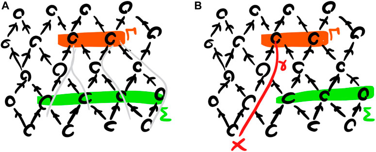
• The category is a poset and the unique morphism from a space-like slice to another space-like slice is denoted if it exists. Specifically, we say that if and only if , i.e. iff lies entirely into the future domain of dependence of . See Figures 2, 3 for examples.
• The monoidal product on objects is only defined when and are space-like separated, in which case it is the disjoint union.
• The unit for the monoidal product is the empty space-like slice .
• The partial monoidal product on objects extends to morphisms because whenever and —i.e. whenever and —we necessarily have:
The partial monoidal product is strict, i.e. strictly associative and unital4 when all products are defined. The partial monoidal product is also commutative, i.e. it is symmetric (wherever defined) with an identity as the symmetry isomorphism. The order relation on slices has been defined in such a way as to ensure that the field state local to the codomain slice will be entirely determined by evolution and marginalization of the field state on the domain slice . In particular, the definition is such that any sub-slice necessarily satisfies , since the field state on can be obtained from the field state on by marginalization/discarding. The connection to marginalisation will be discussed in further detail in Section 4.3 below.
FIGURE 2
FIGURE 2. (A): two slices such that . (B): two slices such that , highlighting a past-directed path γ starting from an event of and not intersecting at any point.
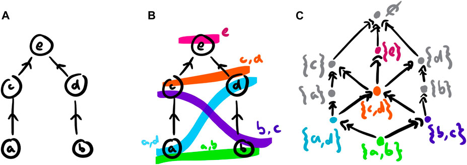
FIGURE 3
FIGURE 3. (A): the Hasse diagram for a causal order. (B): the maximal slices for the causal order highlighted. (C): the category of all slices for the causal order.
2.3 Diamonds and Regions
Definition 13:Let be a causal order. If are two events in , the causal diamond from x to y in is the causal sub-order ↪ defined as follows:
Definition 14:Let be a causal order. A region in is a causal sub-order ↪ which is convex, i.e. one such that for all events the causal diamond from x to y in is a subset of R (i.e. R contains all paths in ).Definition 14 is the order-theoretic incarnation of the requirement that causal diamonds generate the topology of Lorentzian manifolds: we could have equivalently stated it as saying that regions in are all the possibly unions of causal diamonds in (including the empty one). A special case of region of particular interest is the region between two slices .
Definition 15:Let be a causal order and consider two slices . We define the region between and as follows:
In particular, a causal diamond is the region between the slices and . More generally, a region between slices and is the intersection of their future and past respectively. The slices and bounding the region can be obtained respectively as the sets of its minima and of its maxima . As a special case, a slice is the region between and . Conversely, every closed bounded region R—and in particular every finite region—is in the form . See Figure 4 for examples.
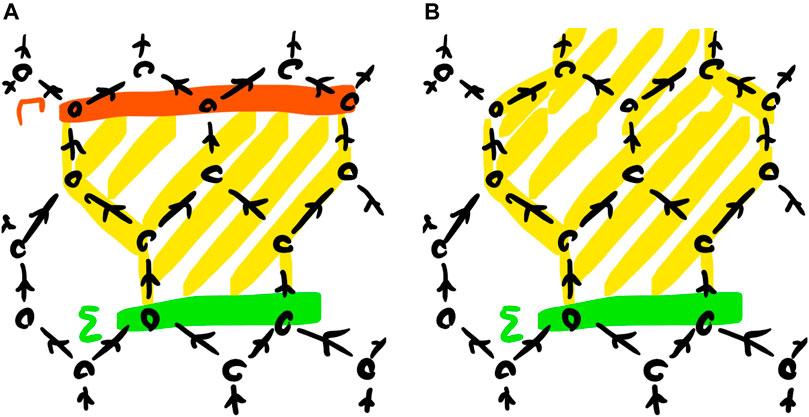
FIGURE 4
FIGURE 4. (A): the region between two slices on the honeycomb lattice. (B): an unbounded (necessarily infinite) region on the honeycomb lattice.
3 Categories of Slices
Because we didn’t impose any topological constraints on the slices, it is possible that the category will, in practice, contain objects which are too irregular or exotic for physical fields to be defined over (such as fractal slices with low topological dimension). To obviate this issue, we consider more general categories of slices on a given causal order: this will allow us to restrict our attention to slices with any properties we desire, as long as we retain enough slices to reconstruct the structure of the causal order , both 1) globally and 2) locally.
No requirement is made for all products that exist in to also exist on members of a more general category of slices: it is the case that certain properties desirable in practice may not be closed under arbitrary union of space-like separated slices themselves satisfying the property.5 However, we impose the requirement 3) that these more general categories of slices be partially monoidal sub-categories of .
Definition 16:Let be a causal order. A category of slices on is the full sub-category of defined by a given set of slices chosen in such a way that the following three conditions hold.
(1) For any two events with , there exist slicessuch that, and .
(2) Ifandare three slices in, then the restrictionofto the regionis also a slice in .
(3) The category of slicesis a partially monoidal subcategory of . In particular, and wheneverexists in for somethenalso exists in (Associativity and unitality of are strict in as they are in ).
In particular, is itself a category of slices on .
Condition (2) in the definition above tells us that we can talk about regions directly within a given category of slices, without first having to reconstruct the causal order : this will form the basis of the connection to AQFT in Section 5 below.
As an example of particularly well-behaved slices, we define a notion of Cauchy slices—akin to that of Cauchy surfaces from Relativity—and remark that any “foliation” of a causal order in terms of such slices gives rise to what is arguably the simplest non-trivial example of category of slices.
Definition 17:A slice on is a Cauchy slice if every causal path in intersects at some (necessarily unique) event. Cauchy slices are in particular maximal slices. A category of Cauchy slices on is a category of slices on such that every slice is a subsetof some Cauchy slice .
Proposition 18:A foliation on a causal order is a set of Cauchy slices on such that:
(1) The slices in are totally ordered according to ;
(2) Every event is contained in some slice ;
(3) The slices in are pairwise disjoint.
If is a foliation, write for the full sub-category of generated by all slices which are subsets of some Cauchy slice in . Then is a category of Cauchy slices on .
Proof: Let denote the full sub-category of generated by all slices which are subsets of some Cauchy slice.
For any two events in , let be two Cauchy slices such that and , the existence of such slices guaranteed by the definition of foliation. Because the foliation is totally ordered, we have that or (or both, if and ). If , either works, while if then necessarily . Either way, condition (1) for to be a category of slices is satisfied.□
Let , and be three slices, respectively contained in three Cauchy slices , and inside the foliation. Because of total ordering and disjointness of slices in , the only instance in which is when . In this case, . Otherwise, . Either way, condition (2) for to be a category of slices is satisfied when , and are Cauchy slices. This result immediately generalises to , and : we have that , so that and condition (2) for to be a category of slices is satisfied.
Finally, if are two slices such that is defined in , then are necessarily disjoint subsets of the same Cauchy slice . It is then immediate to conclude that condition (3) for to be a category of slices is satisfied.
3.1 The category of Causal Orders
As objects, causal orders have been defined simply as posets. However, causal orders are note simply posets, and this should be reflected in the kind of morphisms that can be used to related them to one another. Malament’s result [1] may seem at first to indicate that order-preserving maps are the correct choice, but upon closer inspection one realises that the result itself only talks about order-preserving isomorphisms, giving no indication about other maps.
A prototypical example of the behavior we wish to avoid is that where Ω′ ↪ Ω is a sub-poset such that in for some but in . The issue above is the reason behind the rather specific formulation of the notion of causal sub-order in Definition 2, prompting us to choose a special subclass of order-preserving maps as morphisms between causal orders.
Definition 19:The categoryof causal orders is the symmetric monoidal category defined as follows:
• Objects ofare causal orders, i.e. posets.
• Morphisms in are the order-preserving functionssuch that we have in whenever we have in.
• The monoidal product on objectsis the (forcedly) disjoint union.
• The unit for the monoidal product is the empty causal order .
• The monoidal product extends to the disjoint union of morphisms. If and, then the monoidal productis defined as follows:
The monoidal product is not strict nor commutative, but symmetric under the symmetry isomorphisms defined by. It is easy to check that the causal sub-orders of a causal order according to Definition 2 are all sub-objects Ω′ ↪ Ω in the category , so that the notion of causal sub-order is consistent with the usual notion of categorical sub-object. As discussed above, the regions in a causal order are examples of causal sub-orders, but not all sub-orders are regions: e.g. paths are always sub-orders but not necessarily regions. In general, if we have Ω′ ↪ Ω then it is not necessary for Ω′ to be convex, i.e. it is not necessary for Ω′ to contain all paths x ⇝ y in for any two events Ω′: in the sense, the causal sub-order can “coarsen” the causal order Ω by dropping events “in between” events of the latter. As the following proposition shows, this “coarsening” of causal orders is the only other case we need to consider when talking about causal sub-orders.
Definition 20:Let be a causal order and let the morphism i : Ω′ ↪ Ω be a causal sub-order of . We say that the morphism i : Ω′ ↪ Ω is a region if the image is a region in . We say that the morphism i : Ω′ ↪ Ω is a coarsening if the image is such that for all there exist Ω′ with .
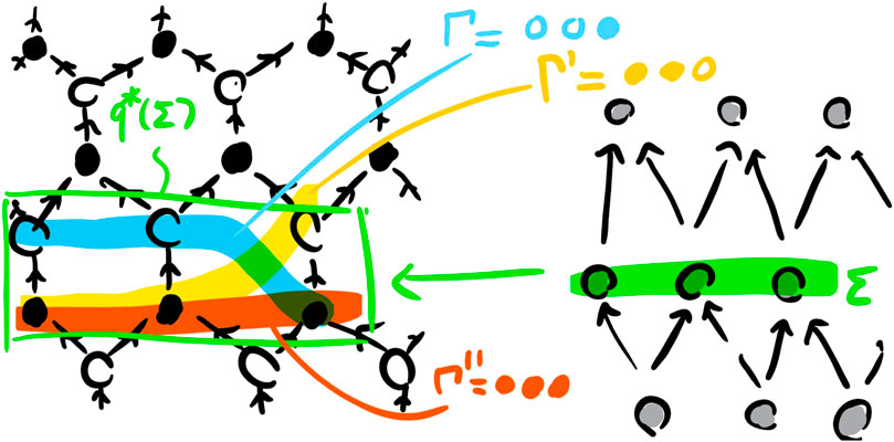
Proposition 21:Let be a causal order and let i : Ω′ ↪ Ω be a causal sub-order of . Then i factors (essentially) uniquely as for some region r : Θ ↪ Ω and some coarsening f : Ω′ ↪ Θ. Proof: Let be the region of obtained as the union of the causal diamonds for all . Let r : Θ ↪ Ω be the injection of into as a sub-poset and let f : Ω′ ↪ Θ be the restriction of the codomain of i to : clearly , r is a region and f is a coarsening (because of how was constructed). Now let Θ′ be such that r′ : Θ′ ↪ Ω is a region and f′ : Ω′ ↪ Θ′ is a coarsening with : to prove essential uniqueness, we want to show that there is some isomorphism such that and . Because , the image is the region itself, so that the restriction of the codomain of to is an isomorphism with . Now we have : but r is a monomorphism (i.e. it is injective), so necessarily .□ The category also has epi-mono factorization, i.e. every morphism can be factorised (essentially) uniquely as an epimorphism (i.e. a surjective map) and a monomorphism (i.e. an injective map) i : Θ ↪ Ω. We have already adopted the nomenclature of causal suborder for the latter form of morphism, while we will henceforth use causal quotient to refer to the former. Causal quotients are surjective morphisms which “collapse” several events into one, in a way which respects the causal order: as an example, a snippet of the causal quotient from the (infinite) honeycomb lattice to the (infinite) diamond lattice is shown in Figure 5. If is a slice in , we can define its pullback to be the causal suborder of generated by , i.e. largest causal sub-order of mapped onto . The pullback of a slice has a rather simple structure: the slices in the pullback are exactly the disjoint unions for all possible choices of slice sections of f over the individual events x of .
A depiction of the pullback under the causal quotient described above can be seen in Figure 6. If is a category of slices on , we can define its pullback along f to be the full sub-category of spanned by all slices in such that for some . The relationship between slices in pullbacks is a little complicated and its full characterization is left to future work.
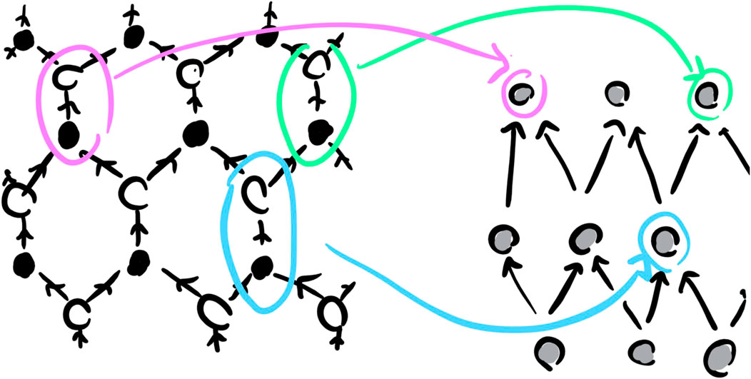
FIGURE 5
FIGURE 5. Causal quotient from the honeycomb lattice to the diamond lattice. The pre-images of three events from the diamond lattice are highlighted.
FIGURE 6
FIGURE 6. A slice on the diamond lattice and three maximal slices , and in its pullback on the honeycomb lattice.
Remark 22:The two notions of pullback defined above—for slices and for categories of slices—are related by the observation that for any slice of (which can equivalently be seen as a causal sub-order Σ ↪ Ω).
4 Casual Field Theories
In the previous Section, we have defined several commonplace notions from Relativity in the more abstract context of causal orders. In this Section, we endow our causal order with fields, living in an appropriate symmetric monoidal category.
4.1 Categories for Quantum Fields
Depending on the specific applications, there are many symmetric monoidal categories available to model quantum fields.
• If the context is finite-dimensional, quantum fields can be taken to live in the category of finite-dimensional Hilbert spaces and completely positive maps between them.
• If the context is finite-dimensional and super-selected systems are of interest, quantum fields can be taken to live in the category of finite-dimensional C*-algebras and completely positive maps between them.
• If the context is finite-dimensional, an even richer playground available for quantum fields is the category : this is the Karoubi envelope of the category , containing and a number of other systems of operational interest (such as fixed-state systems and constrained systems, see e.g. [23]).
• If the context is infinite-dimensional, e.g. in the case of AQFT [10, 11], the categories usually considered for quantum fields are the category of Hilbert spaces and bounded linear maps, the category of C*-algebras and its subcategories of W*-algebras (sometimes known as “abstract” von Neumann algebras) and of (concrete) von Neumann algebras.
• The categories , , and have some annoying limitations, so in an infinite-dimensional context one can alternatively work with hyperfinite quantum systems [24], which incorporate infinities and infinitesimals to offer additional features—such as duals, traces and unital Frobenius algebras—over plain Hilbert spaces and C*-algebras.
The framework we present here is agnostic to the specific choice of process theory (aka symmetric monoidal category) for quantum fields. In fact, it is agnostic to the specific physical theory considered for the fields: any causal process theory can be considered.
4.2 Causal Field Theories
Definition 23:Let be a causal order. A causal field theoryon is a monoidal functorfrom a category of slices on to some symmetric monoidal category , which we refer to as the field category.
Remark 24:It may sometimes be desirable to add a requirement of injectivity on objects for the functor . This has two main motivations, one of physical character and one of mathematical character. Physically, injectivity means that the field spaces corresponding to distinct events have distinct identities (although they can be isomorphic). Mathematically, injectivity means that the image of the functor is itself a sub-category of , matching the style used by other works on compositional causality [8, 19, 20, 23]. While we do not require this as part of our definition, we will take care for the constructions hereafter to be sufficiently general to accommodate the possibility that such a requirement be imposed. We now ask ourselves: what physical information does the functor encode? On objects, associates each space-like slice to the space of fields over that slice: every point in is a valid initial condition for field evolution in the future domain of dependence for .
Remark 25:If is finite and the singleton slices for the individual events are all in the chosen category of slices, then the action of on always factorizes into the tensor product of its action on the individual events:
On morphisms, associates to a morphism : this is a specification of how the field evolves from to , i.e. this defines the map sending a field state over the initial slice to the evolved field state over the final slice . This identification of functorial action with field evolution is the core idea of our work. In particular, it explains our specific definition of morphisms in , and hence in all categories of slices: if and only if the field data on is sufficient to derive the field data on , assuming causal field evolution. Monoidality of the functor on objects says that the space of fields on the union of disjoint slices is the monoidal product—the tensor product, when working in the familiar linear settings of Hilbert spaces, C*-algebras, von Neumann algebras, etc.—of the spaces of fields on the individual slices. Note that this requirement is stronger than the requirement imposed by AQFT, where field algebras over space-like separated diamonds are only required to commute as sub-algebras of the global field algebra, not necessarily to take the form of a tensor product sub-algebra. Functoriality and monoidality on morphisms have some interesting consequences, which we now discuss in detail. Let and for a pair of space-like separated slices and and another pair of space-like separated slices and . Consider the field evolution between the two disjoint unions of slices:
Monoidality on morphisms implies that the field evolution above factors as the product of the individual field evolutions and :
This may look surprising at first, but it becomes entirely natural upon observing the following.
Proposition 26:Let be a causal order. If andare space-like separated slices in and , then andare also space-like separated slices. Proof: If and are space-like separated, then . Because , furthermore, Proposition 9 tells us that . We conclude that , i.e. that and are also space-like separated.□ Proposition 26 above tells us that in our factorization scenario the entire region between and on one side and the entire region between and on the other side are space-like separated. Thus any causal field evolution from to would physically be expected to factor: this can be seen as a manifestation of the principle of locality for field theories, sometimes also known as “clustering.”
Remark 27:Please note that the principle of locality obtained above only implies that the evolution of fields must factorize over space-like separated regions. This imposes no constraints on the field state, which can be any state of the space of fields. In particular, if the field category has entanglement (e.g., categories of Hilbert spaces with the usual tensor product) then the field state can entangle space-like separated regions, while field evolution cannot.
4.3 Causality and No-Signalling
Because any category of slices on a causal order is a partially monoidal subcategory of , in particular it necessarily contains the empty slice (the monoidal unit). We define the following family of effects, indexed by all slices :
By monoidality we have that is some scalar in the field category and that the family respects the partial monoidal structure:
By functoriality, furthermore, the family of effects above is respected by the image of the functor:
This means that the family of effects defined above is an environment structure and that—as long as injectivity of is imposed—the image of the causal field theory is a causal category [19, 20].6 Physically, this means that the field evolution happens in a no-signalling way: if the effects are used as discarding maps—generalizing the partial traces of quantum theory—then the field state over a given slice does not depend on the field state over slices which are in the future of or are space-like separated from .
This emergence of causality and no-signalling from functoriality is in fact a consequence of a breaking of time symmetry which happened in the very definition of the ordering between slices. Indeed, consider the “time-reversed” causal order , obtained by reversing all causal relations in (i.e. in if and only if in ). The slices for are exactly the slices for , i.e. the categories of all slices and have the same objects. If time symmetry were to hold, we would expect the arrows in to be exactly the reverse of the arrows in . However, the conditions defining the arrows in both categories are as follows:
• in iff in ;
• in iff in , i.e. iff in .
The two conditions that and , both in , are not in general equivalent: this shows that time symmetry is broken by our definition of the relationship between slices, ultimately leading to the emergence of causality and no-signalling constraints on functorial evolution of quantum fields.
5 Connection With Algebraic Quantum Field Theory
The definition of causal field theories looks somewhat similar to that of Topological Quantum Field Theories (TQFTs) as functors from categories of cobordism to categories of vector spaces. The big difference between the causal field theories we defined above and TQFTs is that the latter take the basic building blocks for field theories to be defined over arbitrary topological spacetimes, while the former define the evolution over a single given spacetime. This difference is an aspect of a general abstract duality between compositionality and decompositionality.
In compositionality, larger objects are created by composing together given elementary building blocks in all possible ways: this is the approach behind an ever growing zoo of process theories (e.g., see [25] and references therein). In decompositionality, on the other hand, larger objects are given as a whole and subsequently decomposed into smaller constituents, with composition of the latter constrained by the context in which they live: this approach, based on partially monoidal structure, was recently introduced by [22] as a way to talk about compositionality in physical theories where a universe is fixed beforehand. While TQFTs are compositional [13, 26], causal field theories are more naturally understood from the decompositional perspective.
In fact, decompositionality is the key ingredient in a completely different family of approaches to quantum theory, including Algebraic Quantum Field Theory (AQFT) [10] and the topos-theoretic approaches [11, 12]. In AQFT, the relationship between fields and the topology of spacetime is encapsulated into the structure of a presheaf, having as its domain the poset formed by causal diamonds in Minkowski space under inclusion and as its codomain a category of C*-algebras and *-homomorphisms. Specifically, each region (causal diamond) of Minkowski spacetime is mapped to the C*-algebra of “local” quantum observables (categorically: effects) on that region. From this perspective, locality and causality are formulated as the requirement that algebras of local observables over space-like separated regions commute within the algebra of global observables (that is, local effects cannot be entangling over space-like separated regions).
To understand the decompositional character of causal field theories, we draw inspiration from the AQFT approach and turn our functors, defined on slices, into presheafs defined on “regions” (generalising unions of causal diamonds in AQFT). However, our approach differs from the AQFT approach in a number of ways:
• We dispense of the algebras themselves: as mentioned earlier in Section 4.1, our approach is independent of the specific process theory chosen for the fields.
• Instead of looking at the space of local observables/effects, we take the (equivalent) dual perspective and work with the space of local states.
• Local states can be entangling, so the formulation of locality and causality as “commutativity” is no longer applicable, even in the case where the field category is a category of C*-algebras. Instead, locality and causality arise as a consequence of factorization of field evolution over space-like separated slices.
We begin by showing that categories of slices can be restricted to regions, as long as we take care to define regions in such a way as to respect the restrictions imposed by a specific choice of category of slices.
Definition 28:A bounded region in a category of slices on a causal order is a region on in the form for some . Bounded regions in form a poset under inclusion.
Definition 29:A region in a category of slices is a region R on which can be obtained as a union of a family , closed under finite unions, of bounded regions in . Regions in also form a poset under inclusion, with as a sub-poset. Note that if then the regions in are exactly the regions on : by definition, a region R on is the union of the bounded regions for all .
Proposition 30:Let be a category of slices and R be a region in it. The restriction of to the region R, defined as the full sub-category of spanned by the slices such that , is itself a category of slices. Proof: If is a bounded region in , then the statement is an immediate consequence of requirement (2) for categories of slices. Now assume that is a union of bounded regions in . If are two events in R, then it must be that and for some : closure under union of the family then guarantees that there exists some with . Because is a category of slices, we can find two slices in such that and . Then the restrictions and satisfy requirement (1) for to be a category of slices. If , and are three slices in , then in particular the diamond is a subset of R (the latter is a region) and so is the intersection , which exists in because the latter is a category of slices. Hence requirement (2) for to be a category of slices is satisfied. Requirement (3) for to be a category of slices is satisfied, because if then also whenever the latter is defined.□ Given a causal field theory , the restrictions are again causal field theories. To match the spirit of AQFT, we need two more ingredients: the definition of a space of states over a region R and the definition of restrictions between spaces of states associated with inclusions of regions.
Definition 31:Given a region R in a category of slices , the space of states over the region is defined to be the set comprising all families ρ of states over the slices in which are stable under the action of, i.e. comprising all the families
such that for all with the following condition is satisfied:
Bywe have denoted the states on the object of the symmetric monoidal category, i.e. the homsetwhereIis the monoidal unit of.
Proposition 32:Given a causal field theory, we can construct a presheafby associating each regionto the space of statesover the region, and each inclusionto the restriction functiondefined by sending a familyto the familygiven as follows:
We refer toas the presheaf of states over regions of. Proof: The only thing to show is functoriality of . If is the identity on a region R, then we have:
i.e. is the identity on the space of states over the region. If now and , then and we have:
Hence is a presheaf .□
Definition 33:A global state ρ for a causal field theoryis a global compatible family for , i.e. a family such that for all inclusions in . We refer to the set of all global states as the space of global states.
Remark 34:If is a region in , i.e. if , then the states in ( as a region) are in bijection with the global states as follows:
Because of this, we consistently adopt the notation to denote the space of global states. If R is a region in , we also adopt the notation for the map sending a global state to its component over the region R. To unify notation, we will also adopt to denote , taking the same value for any region R containing (e.g., for ).
Remark 35:If the field category is suitably enriched (e.g., in a category with all limits), then a natural choice is for the the space of states to be defined by a presheaf valued in the enrichment category. For example, quantum theory is enriched over positive cones, i.e. -modules, and the -linear structure of states in quantum theory extends to a -linear structure on the spaces of states of causal field theories having quantum theory as their field category. We will not consider such enrichment in this work, though all constructions we present can be readily extended to such a setting. Spaces of states according to Definition 31 encode a lot of redundant information, because we don’t want to look into the specific structure of regions. However, there are certain special cases in which an equivalent description of the space of states over a region can be given.To start with, consider two slices and note that the state on any slice in a bounded region is uniquely determined by applying to the state on :
This is, for example, the case for all bounded regions between Cauchy slices in a category of slices generated by some foliation . If the foliation has a minimum —an initial Cauchy slice—then any global state is entirely determined by its component over the initial slice :
for any and any region R in such that . This extends to all slices in by restriction. Inspired by Relativity, we would like the state on any Cauchy slice in the foliation to determine the global state, not only that on an initial Cauchy slice (which may not exist). For this to happen, we need to strengthen our requirements on the causal field theory, which needs to be causally reversible.
Definition 36:Let be any causal order. By the causal reverse of we mean the causal order on the same events as and such that in if and only if in .
Definition 37:A category of slices on a causal order is said to be causally reversible if the full sub-category of spanned by is a category of slices on the causal reverse . If this is the case, we write for said category of slices over and refer to it as the causal reverse of . We write for the morphisms of .
Definition 38:Letbe a causal field theory on a causal order . If is causally reversible, a causal reversal of is a causal field theory such that:
(1) The functorsandagree on objects, i.e. for allwe have that;
(2) Whenever we have two chains of alternating morphisms in and which start and end at the same slices, say in the form
for some , the composition of the images of the morphisms underandalways yield the same morphism:
We say that is causally reversible—or simply reversible—if is causally reversible and admits a causal reversal.
Proposition 39:Letbe the category of slices on a causal ordergenerated by some foliation. Thenis always causally reversible and for any two Cauchy slices we have thatif and only if. Furthermore, if a causal field theoryis reversible, then a global state ρ is entirely determined by the stateon any Cauchy slice as follows:
whereis any causal reversal of. Proof: The main observation behind this result is as follows: if are two Cauchy slices, then the conditions and are equivalent. Hence is always causally reversible and if and only if for any two Cauchy slices . Now let be causally reversible, let be a Cauchy slice in the foliation and consider any global state ρ. If for some other Cauchy slice , then the definition of a global state implies that . If instead , then and the definition of a global state implies that . But the definition of a causal reverse also implies that:
Hence the value completely determines the global state ρ (since the value on all other slices in is determined by restriction from the value on a corresponding Cauchy slice).□ It is an easy check that not only the global states are determined—under the conditions of Proposition 39—by their component over any Cauchy slice in the foliation, but also that Eq. 29 can be used—under the same conditions—to construct a global state from a state on any Cauchy slice in the foliation. Before concluding this Section, we would like to remark that a succinct description of spaces of states over regions can be obtained in settings much more general than those of foliations: for example, in all those cases where the every region admits a suitable Cauchy slice and the causal field theory is reversible. The careful formulation of this more general setting is key to the further development of the connection between causal field theory and AQFT and it is left to future work.
6 Connection to Quantum Cellular Automata
The idea of a cellular automaton was first introduced by von Neumann, aimed at designing a self replicating machine [18]. A Cellular Automaton (CA) over some finite alphabet A has its state stored as a d-dimensional lattice of values in A, i.e. as a function . The state is updated at discrete time steps, each step updated as according to some fixed function . The function F acts locally and homogeneously: there is some fixed finite subset (typically a neighborhood of ) and some function such that the value of each lattice site at time step only depends on the finitely many values in the subset at time t:
A Quantum Cellular Automaton (QCA) is a generalization of a CA where the lattice states are replaces by (pure) states in the tensor product of Hilbert spaces (all finite-dimensional and isomorphic) and the function F is replaced by a unitary , with requirements of locality and homogeneity.
Remark 40:There are several slightly different formulation of the infinite tensor product above that can be used, each with its own advantages and disadvantages: though it is not going to be a concern for this work, the authors are partial to the construction by von Neumann [27]. An early formulation of the notion of QCA is due to Richard Feynman, in the context of simulations of physics using quantum computers [28]. More recent work on quantum information and quantum causality has shown that the evolution of certain free quantum fields can be recovered as the continuous limit of certain quantum cellular automata (cf [16, 17]. and references therein). In the final section of this work, we show that our framework is well-suited to capture notions of QCA such as those appearing in the literature. Specifically, our construction encompasses and greatly generalises that presented in [17].
6.1 Causal Cellular Automata
The first requirement in the definition of a QCA is that of homogeneity—called “translation invariance” in [17]—i.e. the requirement that the automaton act the same way at all points of spacetime. Because presentations of QCAs are usually given in terms of discrete updates of states on a lattice by means of a unitary U, only the requirement of homogeneity in space is usually mentioned. However, such presentations also have homogeneity in time as an implicit requirement, namely in the assumption that the same unitary U be used to update the state at all times.
Instead of updating the state time-step by time-step in a compositional fashion, our formulation of quantum cellular automata will see the entirety of spacetime at once, with states over slices and regions recovered in a decompositional approach. Nevertheless, the requirement of homogeneity for a QCA can still be formulated as a requirement of invariance under certain symmetries of spacetime, so we begin by formulating such a notion of invariance for causal field theories.
Definition 41:A symmetry on a causal order is an action of a group G on by automorphisms of causal orders, i.e. a group homomorphism . If is a category of slices on , a symmetry on is a symmetry on which extends to an action on by partially monoidal functors, i.e. one such that the following conditions are satisfied:
(1) for all , ifthen;
(2) for all and all, ifthen;
(3) for all and all, ifis defined in then is also defined in.
Note, for all , that and thatis automatically a slice wheneveris a slice.
Definition 42:Let be a category of slices with a symmetry action of a group G. A G-invariant (or simply symmetry-invariant) causal field theory on is a causal field theoryequipped with a family of natural isomorphismssuch that , where we have identified elements with their action as partially monoidal functors .
Remark 43:The spirit behind the definition of symmetry-invariant causal field theories is that the functors(sending slices fields) and (sending slices g-translated slices fields) should be the same. However, we have remarked when first defining causal field theories that—be it for ease of physical interpretation or for conformity with existing literature on causal categories—it may sometimes be desirable that the imagesof different slices be different. Not being able to impose the equalityin such a setting, the next best thing is to ask for natural isomorphism. Because we are dealing with symmetries, however, it is sensible to require for the natural isomorphisms themselves to respect the group structure. Again, the first instinct might be to require something in the form , but this expressions does not type-check: we have a natural transformation , a natural transformationand a natural transformation. In order to compose and we instead have to take the action of translated to:
Explicitly, the natural transformation is defined by. The second requirement in the definition of a QCA is that of locality (or causality). When quantum cellular automata are considered in a relativistic context—e.g. as discrete models of quantum field theories—the requirement of locality is meant to capture the idea that the action of the automaton should respect the causal structure of spacetime (so that the state on a point at time should not depend on the state at the previous time t on points which are “too far away”, i.e. such that and are space-like separated). In [17], the requirement of locality is formulated as the requirement that the output state of the automaton over a point of the lattice at time only depend on the state over a finite neighborhood at time t: this is both in terms of local state (causality) and in the stronger sense that the field evolution should factor into a product of local maps (localisability). In our framework, on the other hand, causality and localisability are both automatically enforced: the field evolution always factors over space-like separated regions, as a consequence of monoidality, and the local state over a slice never depends on the state on any other slice which is space-like separated from it (as a consequence of factorisation).
Remark 44:The causal order which captures the causality requirement from [17] with finite neighborhood can be constructed by endowing the set with the reflexive-transitive closure of the relation for all times , for all points of the lattice and for all points in the neighborhood of . The third and final requirement in the definition of a QCA is that of unitarity. In our framework, this is a problem for two (mostly unrelated) reasons.
• Our formulation of causal field theories aims to be agnostic to the choice of process theory. On the other hand, unitarity is a strongly quantum-like feature, the formulation of which would require a significant amount of additional structure on the field category.
• The usual formulation of quantum cellular automata only considers global evolution, never directly dealing with restrictions—situations e.g., in which the state is evolved unitarily but part of the output state is discarded as environment. Our framework instead treats such restrictions as an integral part of evolution.
Luckily, unitarity per se is not necessary from an abstract foundational standpoint: the real feature of interest is reversibility, a feature of causal field theories which we have already explored. For the sake of generality, we will not include reversibility in the definition below, leaving it as an explicit desideratum.
Remark 45:In categories of Hilbert spaces and completely positive maps, it is legitimate to imagine that causality and reversibility would jointly imply that the cellular automata also be unitary. This is indeed the case under the conditions of Proposition 39: because the state on any Cauchy slice automatically determines the state on all the other slices—and because that state on a single slice is arbitrary—evolution between Cauchy slices must be unitary.
Definition 46:A Causal Cellular Automaton (CCA) consists of the following ingredients.
(1) A foliation on a causal order .
(2) A category of Cauchy slices such that each slice in is a subset of some Cauchy slice in .7
(3) A symmetry action of a group G on , inducing—via the G-action on —a transitive action of G on the Cauchy slices in the foliation .
(4) A G-invariant causal field theory.
A reversible CCA is one where the causal field theoryis reversible.Definition 46 is much more general than the definition of QCA from [17] and hence captures more sophisticated examples. However, its ingredients are directly analogous to those appearing in that definition of a QCA.
• The foliation on generalizes the discrete time steps in the definition of a QCA.
• The slices in generalize the equal-time hyper-surfaces which support the state of a QCA at fixed time.
• The symmetry action of G on and its transitivity on the foliation generalise homogeneity in both space and time of the lattices supporting a QCA.
• The G-invariance of the causal field theory generalizes both the translation symmetry in space and the time-translation symmetry of a QCA.
A different approach to QCAs in non-homogeneous space-times appears in [29, 30], in terms of graph dynamics. The graph dynamics models and the models described in this work present a significant overlap—in the specific case of quantum theory—but are ultimately incomparable: on the one end, graph dynamics impose certain structural requirements on spacetime slices for the foliation, requirements which are not necessary in this work; on the other end, quantum graph dynamics allow a superposition of graphs at each slice of the foliation, a possibility which is not considered in this work.
6.2 Partitioned Causal Cellular Automata
We now proceed to construct a large family of examples of CCAs based on the partitioned QCAs of [17]. In doing so, we generalise the scattering unitaries to arbitrary processes and allow for the definition of state restriction to non-Cauchy equal-time surfaces. We refer to the resulting CCA as partitioned CCA.
6.2.1 Causal Order
As our causal order we consider the following subset of -dimensional Minkowski spacetime (setting the constant c for the speed of light to ):
where is the set of all such that . For we get the -dimensional diamond lattice discussed before. In general, the immediate causal predecessors of a point are the following points:
where we defined the “neighborhood” . Similarly, the immediate successors of are the following points:
6.2.2 Foliation and Category of Slices
The causal order admits a foliation where each slice is a constant-time Cauchy slice for some :
A suitable category of slices to associate to this foliation is given by taking as slices all the finite sets of events having the same time coordinate t:
where is some finite subset. The morphisms of are given as follows for :
where the “iterated neighborhood” is defined as by adding together copies of (and we set ). Explicitly we have:
It is easy to check (by a symmetry argument) that is reversible.
6.2.3 Symmetry
The category admits a symmetry action of the group . We index the coordinates of vectors in by the points . We denote by the vector in which is 1 at the coordinate labeled by and 0 at all other coordinates. The action is then specified by setting:
that is, the generators of send a generic event to each of its immediate causal successors in , one for each possible choice of sign along each of the d directions of the space lattice .8 Each generator for the symmetry action sends a Cauchy slice in the foliation to the next Cauchy slice , so the action of G on the foliation is transitive.
6.2.4 Causal Field Theory—Field Over Slices
As our field category we consider a generic causal process theory, i.e. a symmetric monoidal category equipped with a family of discarding maps for all objects , respecting the tensor product and tensor unit I of : and . Discarding maps generalize the partial trace of quantum theory: normalized states —generalizing density matrices—are defined to be those such that and normalized morphisms —generalizing CPTP maps—are defined to be those such that . See e.g. [20, 23, 25] for more information.
To create a G-invariant causal field theory , we consider some object together with some endomorphism , which we will refer to as the scattering map. For reasons that will soon become clear, it is more convenient to index the factors of by the points in the neighborhood , hence writing .
We define the action of on the slices in as follows:
The tensor product is well-defined in all symmetric monoidal categories, since is always finite. Physically, the field takes values in a copy of over each event of spacetime, each individual factor of encoding the contribution to the field state at from the field state at each of its immediate causal predecessors in .
6.2.5 Causal Field Theory - Restriction and Evolution
From their definition in Eq. 38, it is easy to see that morphisms on can always be factored in the following way:
where for all and the following holds for each :
This means that we only need to care about the action of on two kinds of morphisms:
• The restrictions , where ;
• The 1-step evolutions , where .
The existence of the factorisation above can be proven by induction, observing that any morphism factors into the product:
where is defined as before so that is exactly the set of immediate causal predecessors of the codomain .
On restrictions , where , the functor is defined to act by marginalization, discarding the field state over all those events in the larger slice which don’t belong to the smaller slice :
On 1-step evolutions , where , the functor is defined to act by a combination of evolution by U and marginalization. The evolution component is simply an application of U to the state at each event of :
The marginalization component then needs to go from the codomain of the map above to the desired codomain . To do this, we recall that the factor of corresponding to a given and a given is intended to encode the component of the state at coming from . Analogously, the factor of corresponding to a given and a given is intended to encode the component of the evolved state going to . Hence to go from to we need to discard all factors in corresponding to components of the evolved state which are not going to some :
Putting the evolution and marginalization components together we get the action of on 1-step evolutions:
By construction, the above is a G-invariant causal field theory, completing the definition of our partitioned causal cellular automaton. If U is an isomorphism, the same construction on using provides a causal reversal for , showing that the partitioned causal cellular automaton above is reversible under those circumstances. Finally, Figure 7 below depicts an example of action on morphisms for a -dimensional partitioned causal cellular automaton.
FIGURE 7
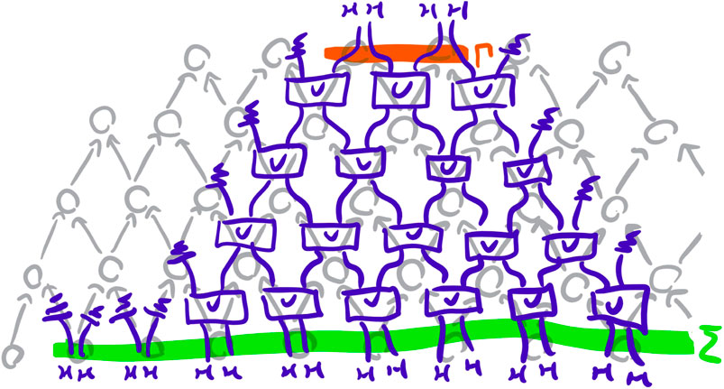
FIGURE 7. Action of a partitioned causal cellular automaton over a complicated morphism in the -dimensional example of the diamond lattice. Here , so each event in the causal order is associated to a copy of . The restriction action of the CCA (Eq. 45) can be seen on the two events at the bottom left. The pure evolution action of the CCA (Eq. 46) can be seen on the central pyramid of ten events, as the application of U without discarding. The evolution + marginalisation action of the CCA (Eq. 48) can be seen on the eight events at the sides of the central pyramid, as the application of U followed by discarding of one of the two outputs. The input of the morphism depicted consists of eight copies of , one for each event of , while the output of the morphism depicted consists of two copies of , one for each event of .
6.3 Sketch of the Continuous Limit for the Dirac Quantum Cellular Automata
To conclude, we note how in [17] it is argued that the Dirac equation for free propagation of an electron can be recovered in the continuous limit of a specific -dimensional partitioned QCA. The original argument could not be made fully rigorous, because the QCAs defined therein were discrete and no setting was available to the author in which to make proper sense of the infinite tensor product arising from the limiting construction. A rigorous analysis of the limit is presented in [31], but the limit itself exists outside of the QCA framework.
Our definition of CCA, on the other hand, has no requirement of discreteness. Furthermore, the freedom left in the choice of field category for a CCA allows us to benefit from the full power of the non-standard approach to categorical quantum mechanics [24, 32]. As a consequence, we are able to sketch below a formalization within our framework of the continuous limit for the Dirac QCA, following the same lines as the construction of a -dimensional partitioned CCA above.
The key to obtain a continuous limit for the Dirac QCA is to rescale the discrete lattice to one with infinitesimal mesh ε:
where are the non-standard integer numbers. The slices are now allowed to contain an infinite number of points and can be used to approximate all equal-time partial Cauchy hyper-surfaces in -dimensional Minkowski spacetime. Unfortunately, the infinite number of points in our slices now requires infinite tensor products to be taken: to deal with this, we use as our field category the dagger compact category of non-standard hyperfinite-dimensional Hilbert spaces, where such infinite products can be handled safely.
We set the scattering map to be the following non-standard unitary
where is the X Pauli matrix: this is the same unitary used in the Dirac QCA, but with the real parameter ε turned into an infinitesimal. Each application of U only inches infinitesimally further from the identity, but in the non-standard setting we are allowed to consider the cumulative effect across infinite sequences of infinitesimally close slices. The first order approximations to the Dirac equation derived in [17] turn into legitimate infinitesimal differentials, connecting the state on each slice to the state on the (infinitesimally close) next slice: once the standard part is taken, the lattice ends up covering the entirety of -dimensional Minkowski spacetime, the differentials get integrated and turns into a continuous-time field evolution following the Dirac equation.
Remark 47:The power to express limiting constructions algebraically, without exiting the original framework, is one of the most attractive aspects of non-standard analysis. The dagger compact category (and other categories derived from it) can be used to make categorical sense of constructions from quantum field theory [24, 32], including other cellular automata with field-theoretic continuous limits. The formulation of such limits within our framework is an point of great interest, but is left to future work.
7 Conclusion and Future Work
In this work, we have defined a functorial, theory-independent notion of causal field theory founded solely on the order-theoretic structure of causality. We have seen how the causality requirement for such field theories is automatically satisfied as a consequence of symmetry-breaking in the ordering on space-like slices. In an effort to connect to Algebraic Quantum Field Theory (AQFT), we have constructed complex spaces of states over regions of spacetime and discussed how the associated information redundancy can be reduced in selected cases. We have introduced symmetries in our framework and shown that Quantum Cellular Automata (QCA) can be modeled within it, both in their traditional discrete formulation and in their continuous limit.
Despite our efforts, we feel we have barely scratched the surface on the potential of this material. In the future, we envisage three lines of research stemming from this work. Firstly, we believe that the connection with AQFT can be strengthened and honed to the point that the framework will be a tool for the construction of new models. This includes a thorough understanding of the structure of spaces of states for categories of slices more general than those induced by foliations. Secondly, we wish to further explore and fully characterise the possibilities associated with working in the continuous limit of QCAs, with an eye to applications in perturbative quantum field theory. Finally, we plan to extend the framework in a number of directions, including indefinite causal order—already achieved for QCAs by [30], at least in partial form—enrichment and the possibility of working with restricted classes of causal paths (in temporal analogy to categories of slices).
Author Contributions
Research carried out by SG and by MS under the supervision of BC. Writing carried out by SG and MS, with editing by BC. Revision and approval of work carried out by SG, MS, and BC.
Funding
This work is supported by a grant form the John Templeton Foundation. The opinions expressed in this publication are those of the authors and do not necessarily reflect on the views of the John Templeton Foundation. MS is supported by an EPSRC grant, ref. EP/P510270/1.
Conflict of Interest
The authors declare that the research was conducted in the absence of any commercial or financial relationships that could be construed as a potential conflict of interest.
Publisher’s Note
All claims expressed in this article are solely those of the authors and do not necessarily represent those of their affiliated organizations, or those of the publisher, the editors and the reviewers. Any product that may be evaluated in this article, or claim that may be made by its manufacturer, is not guaranteed or endorsed by the publisher.
Footnotes
1The requirement for a manifold M to be future- and past-distinguishing is essentially one of well-behaviour, e.g. excluding causal violations such as closed timelike curves (all points of which necessarily have the same causal past and future).
2The local finiteness condition for a causal set can equivalently be stated as the requirement that the partial order arises as the reflexive-transitive closure of a non-transitive directed graph, its Hasse diagram (see e.g. [8]).
3I.e. such that for all we have that in if and only if in .
5An example of this phenomenon is given by constant-time partial Cauchy slices in Minkowski spacetime: the union of two disjoint constant-time partial Cauchy slices having the same time parameter yields another constant-time partial Cauchy slice, but the union of two space-like separated constant-time partial Cauchy slices having different time parameters does not yield a constant-time partial Cauchy slice as a result.
6We have taken the liberty to extend the definition of environment structures to partially monoidal categories, such as the image of a injective on objects under the partial monoidal product induced by the partial monoidal product of the domain category .
7Each Cauchy slice in is then automatically the union of all slices such that .
8The reason for the negative sign in is that was originally defined to be the neighborhood in the past.
References
1. Malament DB. The Class of Continuous Timelike Curves Determines the Topology of Spacetime. J Math Phys (1977) 18:1399–404. doi:10.1063/1.523436
3. Hawking SW, King AR, McCarthy PJ. A New Topology for Curved Space-Time Which Incorporates the Causal, Differential, and Conformal Structures. J Math Phys (1976) 17:174–81. doi:10.1063/1.522874
4. Martin K, Panangaden P. Domain Theory and General Relativity. In: New Structures for Physics. Berlin, Heidelberg: Springer (2010). p. 687–703. doi:10.1007/978-3-642-12821-9_11
5. Martin K, Panangaden P. Spacetime Geometry from Causal Structure and a Measurement. In: Mathematical Foundations of Information Flow: Clifford Lectures Information Flow in Physics, Geometry, and Logic and Computation; March 12-15, 2008; New Orleans, Louisiana. Tulane University (2012). p. 213. 71.
8. Pinzani N, Gogioso S, Coecke B. Categorical Semantics for Time Travel. In: 34th Annual ACM/IEEE Symposium on Logic in Computer Science (LICS 2019)(IEEE Computer Society) (2019). doi:10.1109/LICS.2019.8785664
12. Doering A, Isham C. What Is a Thing?. In: Topos Theory in the Foundations of Physics. Berlin, Heidelberg: Springer (2008). p. 753–940. doi:10.1007/978-3-642-12821-9_13
14. Atiyah M. Topological Quantum Field Theories. Publications Mathématiques de l'Institut des Hautes Scientifiques (1988) 68:175–86. doi:10.1007/bf02698547
21. Kissinger A, Uijlen S. A Categorical Semantics for Causal Structure. In: 2017 32nd Annual ACM/IEEE Symposium on Logic in Computer Science (LICS). IEEE (2017). p. 1–12. doi:10.1109/LICS.2017.8005095
24. Gogioso S, Genovese F. Quantum Field Theory in Categorical Quantum Mechanics. Electron Proc Theor Comput Sci (2018) 287:163–77. doi:10.4204/EPTCS.287.9
26. Kock J. Frobenius Algebras and 2D Topological Quantum Field Theories. Cambridge, United Kingdom: Cambridge University Press (2003). doi:10.1017/CBO9780511615443
32. Gogioso S, Genovese F. Towards Quantum Field Theory in Categorical Quantum Mechanics. Electron Proc Theor Comput Sci (2017) 266:349–66. doi:10.4204/EPTCS.266.22
Disclaimer: All claims expressed in this article are solely those of the authors and do not necessarily represent those of their affiliated organizations, or those of the publisher, the editors and the reviewers. Any product that may be evaluated in this article or claim that may be made by its manufacturer is not guaranteed or endorsed by the publisher.
 Stefano Gogioso
 Maria E. Stasinou
 Bob Coecke
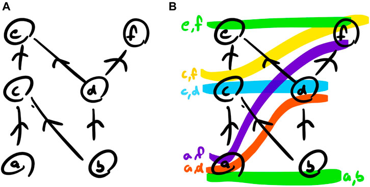

 is some scalar in the field category

 defined above is an environment structure and that—as long as injectivity of
  are used as discarding maps—generalizing the partial traces of quantum theory—then the field state over a given slice
  for all objects
  and
and  . Discarding maps generalize the partial trace of quantum theory: normalized states
  and normalized morphisms
  . See e.g. [20, 23, 25] for more information.