Equivalence of Approaches to Relational Quantum Dynamics in Relativistic Settings

1. Introduction

In general relativity, time plays a different role than in classical and quantum mechanics, or quantum field theory on a Minkowski background. General covariance dispenses with a preferred choice of time and introduces instead a dynamical notion of time which depends on solutions to the Einstein field equations. In the canonical approach to quantum gravity this leads to the infamous problem of time [1–3]. Its most well-known facet is that, due to the constraints of the theory, quantum states of spacetime (and any matter contained in it) do not at first sight appear to undergo any time evolution, in seeming contradiction with everyday experience.

The resolution comes from one of the key insights of general relativity: any physical notion of time is relational, the degrees of freedom of the Universe evolve relative to one another [4–6]. This insight has led to three main relational approaches to the problem of time, each of which seeks to extract a notion of time from within the quantum degrees of freedom, relative to which the others evolve:

(i) a Dirac quantization scheme, wherein relational observables are constructed that encode correlations between evolving and clock degrees of freedom [1, 2, 4, 7–38],

(ii) the Page-Wootters formalism, which defines a relational dynamics in terms of conditional probabilities for clock and evolving degrees of freedom [7, 25, 39– 57], and

(iii) classical or quantum deparametrizations, which result in a reduced quantum theory that only treats the evolving degrees of freedom as quantum [1, 2, 7, 10, 30, 31, 58–65].

These three approaches have been pursued largely independently with the relation between them previously unknown. They have also not been without criticism, especially the Page-Wootters formalism. For example, Kuchař [1] raised three fundamental criticisms against this approach, namely that it:

(a) leads to wrong localization probabilities in relativistic settings,

(b) is in conflict with the constraints of the theory, and

(c) yields wrong propagators.

Concern has also been voiced that there is an inherent ambiguity in terms of which clock degrees of freedom one should choose, also known as the multiple choice problem [1–3, 66, 67]. Indeed, in generic general relativistic systems there is no preferred choice of relational time variable and different choices may lead to a priori different quantum theories.

In our recent work [7] we addressed the relation between these three approaches (i)–(iii) to relational quantum dynamics, demonstrating that they are, in fact, equivalent when the clock Hamiltonian features a continuous and non-degenerate spectrum and is decoupled from the system whose dynamics it is used to describe. Specifically, we constructed the explicit transformations mapping each formulation of relational quantum dynamics into the others. These maps revealed the Page-Wootters formalism (ii) and quantum deparametrizations (iii) as quantum symmetry reductions of the manifestly gauge-invariant formulation (i). In other words, the Page-Wootters formalism (ii) and quantum deparametrizations (iii) can be regarded as quantum analogs of gauge-fixed formulations of gauge-invariant quantities (i). Conversely, the formulation in terms of relational Dirac observables (i) constitutes the quantum analog of a gauge-invariant extension of the gauge-fixed formulations (ii) and (iii). More physically, these transformations establish (i) as a clock-choice-neutral (in a sense explained below), (ii) as a relational Schrödinger, and (iii) as a relational Heisenberg picture of the dynamics. Constituting three faces of the same quantum dynamics, we called the equivalence of (i)–(iii) the trinity of relational quantum dynamics.

This equivalence not only provides relational Dirac observables with a consistent conditional probability interpretation, but also resolves Kuchař's criticism (b) that the Page-Wootters formalism would be in conflict with the quantum constraints. Furthermore, the trinity resolves Kuchař's criticism (c) that the Page-Wootters formalism would yield wrong propagators, by showing that the correct propagators always follow from manifestly gauge-invariant conditional probabilities on the physical Hilbert space [7]. This resolution of criticism (c) differs from previous resolution proposals which relied on ideal clocks [25, 43, 68] and auxiliary ancilla systems [43] and can be viewed as an extension of [46].

The transformations between (i)–(iii) of the trinity also allowed us to address the multiple choice problem in Höhn et al. [7] by extending a previous method for changing temporal reference frames, i.e., clocks, in the quantum theory [30, 31, 47] (see also [32–34, 69]). The resolution to the problem lies in part in realizing that a solution to the Wheeler-DeWitt equation encodes the relations between all subsystems, including the relations between subsystems employed as clocks to track the dynamics of other subsystems; there are multiple choices of clocks, each of which can be used to define dynamics. Our proposal is thus to turn the multiple choice problem into a feature by having a multitude of quantum time choices at our disposal, which we are able to connect through quantum temporal frame transformations. This is in line with developing a genuine quantum implementation of general covariance [7, 30, 31, 38, 70–74]. This proposal is part of current efforts to develop a general framework of quantum reference frame transformations (and study their physical consequences [75–85]), and should be contrasted with other attempts at resolving the multiple choice problem by identifying a preferred choice of clock [53] (see [7] for further discussion of this proposal).

We did not address Kuchař's criticism (a) that the Page-Wootters formalism yields the wrong localization probabilities for relativistic models in Höhn et al. [7] as they feature clock Hamiltonians which are quadratic in momenta and thus generally have a degenerate spectrum, splitting into positive and negative frequency sectors. This degeneracy is not covered by our previous construction. While quadratic clock Hamiltonians are standard in the literature on relational observables [approach (i)] and deparametrizations [approach (iii)], see e.g., [4, 10, 11, 19, 29, 31], relativistic particle models have only recently been studied in the Page-Wootters formalism [approach (ii)] [45, 49–51]. However, Kuchař's criticism (a) that the Page-Wootters approach yields incorrect localization probabilities in relativistic settings has yet to be addressed. Since the Page-Wootters formalism encounters challenges in relativistic settings, given the equivalence of relational approaches implied by the trinity, one might worry about relational observables and deparametrizations too.

In this article, we show that these challenges can be overcome, and a consistent interpretation of the relational dynamics can be provided. To this end, we extend the trinity to quadratic clock Hamiltonians, thus encompassing many relativistic settings; we show that all the results of Höhn et al. [7] hold per frequency sector associated to the clock due to a superselection rule induced by the Hamiltonian constraint. Frequency-sector-wise, the relational dynamics encoded in (i) relational observables, (ii) the Page-Wootters formalism, and (iii) quantum deparametrizations are thus also fully equivalent.

The key to our construction, as in Höhn et al. [7], is the use of a Positive-Operator Valued Measure (POVM) which here transforms covariantly with respect to the quadratic clock Hamiltonian [86–89] as a time observable. This contrasts with the usual approach of employing an operator conjugate to the clock momentum (i.e., the Minkowski time operator in the case of a relativistic particle). This covariant clock POVM is instrumental in our resolution of Kuchař's criticism (a) that the Page-Wootters formalism yields wrong localization probabilities for relativistic systems. We show that when conditioning on this covariant clock POVM rather than Minkowski time, one obtains a Newton-Wigner type localization probability [90, 91]. While a Newton-Wigner type localization is approximate and not fully Lorentz covariant, due to the relativistic localization no-go theorems of Perez-Wilde [92] and Malament [93] (see also [94, 95]), it is generally accepted as the best possible localization in relativistic quantum mechanics (In quantum field theory localization is a different matter [90, 94]). This demonstrates the advantage of using covariant clock POVMs in relational quantum dynamics [7, 44, 45, 96, 97]. The trinity also extends the probabilistic interpretation of relational observables: a Dirac observable describing the relation between a position operator and the covariant clock POVM corresponds to a Newton-Wigner type localization in relativistic settings.

Finally, we again use the equivalence between (i) and (iii) to construct temporal frame changes in the quantum theory. On account of superselection rules across frequency sectors, temporal frame changes can only map information contained in the overlap of two frequency sectors, one associated to each clock, from one clock “perspective” to another. We apply these temporal frame change maps to explore an indirect clock self-reference and the temporal frame and state dependence of comparing and synchronizing readings of different quantum clocks.

While completing this manuscript, we became aware of Chataignier [38], which independently extends some results of Höhn et al. [7] on the conditional probability interpretation of relational observables and their equivalence with the Page-Wootters formalism into a more general setting. However, a different formalism [37] is used in Chataignier [38], which does not employ covariant clock POVMs and therefore the two works complement one another.

Throughout this article we work in units where ℏ = 1.

2. Clock-Neutral Formulation of Classical and Quantum Mechanics

Colloquially, general covariance posits that the laws of physics are the same in every reference frame. This is usually interpreted as implying that physical laws should take the form of tensor equations. Tensors can be viewed as reference-frame-neutral objects: they define a description of physics prior to choosing a reference frame. They thereby encode the physics as “seen” by all reference frames at once. If one wants to know the numbers which a measurement of the tensor in a particular reference frame would yield, one must contract the tensor with the vectors corresponding to that choice of frame. In this way, the description of the same tensor looks different relative to different frames, but the tensor per se, as a multilinear map, is reference-frame-neutral. It is this reference-frame-neutrality of tensors which results in the frame-independence of physical laws.

The notion of reference frame as a vector frame is usually taken to define the orientation of a local laboratory of some observer. In practice, one often implicitly identifies the local lab (i.e., the reference system relative to which the remaining physics is described) with the reference frame. This is an idealization which ignores the lab's back-reaction on spacetime, interaction with other physical systems and possible internal dynamics, while at the same time assuming it to be sufficiently classical so that superpositions of orientations can be ignored. Such an idealization is appropriate in general relativity where the aim is to describe the large-scale structure of spacetime. However, in quantum gravity, where the goal is to describe the micro-structure of spacetime, this may no longer be appropriate [98]. More generally, we may ask about the fate of general covariance when we take seriously the fact that physically meaningful reference frames are in practice always associated with physical systems, and as such are comprised of dynamical degrees of freedom that may couple with other systems, undergo their own dynamics and will ultimately be subject to the laws of quantum theory. What are then the reference-frame-neutral structures?

In regard to this question, we note that the classical notion of general covariance for reference frames associated to idealized local labs is deeply intertwined with invariance under general coordinate transformations, i.e., passive diffeomorphisms. In moving toward non-idealized reference frames (or rather systems), we shift focus from coordinate descriptions to dynamical reference degrees of freedom, relative to which the remaining physics will be described. In line with this, we shift the focus from passive to active diffeomorphisms, which directly act on the dynamical degrees of freedom. This is advantageous for quantum gravity, where classical spacetime coordinates are a priori absent. A quantum version of general covariance should be formulated in terms of dynamical reference degrees of freedom [7, 30, 31, 38, 70–74].

The active symmetries imply a redundancy in the description of the physics. A priori all degrees of freedom stand on an equal footing, giving rise to a freedom in choosing which of them shall be treated as the redundant ones. The key idea is to identify this choice with the choice of reference degrees of freedom, i.e., those relative to which the remaining degrees of freedom will be described¹. Accordingly, choosing a dynamical reference system amounts to removing redundancy from the description. As such, we may interpret the redundancy-containing description (in both the classical and quantum theory) as a perspective-neutral description of physics, i.e., as a global description of physics prior to having chosen a reference system, from whose perspective the remaining degrees of freedom are to be described [7, 30, 31, 71, 72]. This perspective-neutral structure is thus proposed as the reference-frame-neutral structure for dynamical (i.e., non-idealized) reference systems.

In this article we focus purely on temporal diffeomorphisms and thus on temporal reference frames/systems, or simply clocks. In this case, we refer to the perspective-neutral structure as a clock-(choice-)neutral structure [7, 30, 31], which we briefly review here in both the classical and quantum theory. It is a description of the physics, prior to having chosen a temporal reference system relative to which the dynamics of the remaining degrees of freedom are to be described.

2.1. Clock-Neutral Classical Theory

Consider a classical theory described by an action ${S}={\int }_{ℝ}duL(q^a,d{q}^a/du)$, where q^a denotes a collection of configuration variables indexed by a. Such a theory exhibits temporal diffeomorphism invariance if the action ${S}$ is reparametrization invariant; that is, L(q^a, dq^a/du) ↦ L(q^a, dq^a/du′)du′/du transforms as a scalar density under u ↦ u′(u). The Hamiltonian of such a theory is of the form H = N(u)C_H, where N(u) is an arbitrary lapse function and

$\begin{array}{ll}{C}_H={\displaystyle \sum _a}\frac{d{q}^a}{du}{p}_a-L\approx 0,& (1)\end{array}$

the so-called Hamiltonian constraint, is a consequence of the temporal diffeomorphism symmetry. This equation defines the constraint surface ${C}$ inside the kinematical phase space ${{P}}_{\text{kin}}$, which is parametrized by the canonical coordinates $q^a,p_b$. The ≈ denotes a weak equality, i.e., one which only holds on ${C}$ [101, 102].

The Hamiltonian generates a dynamical flow on ${C}$, which transforms an arbitrary phase space function f according to

$\begin{array}{ll}\frac{df}{du}≔\left\{f,C_H\right\}& (2)\end{array}$

and integrates to a finite transformation ${\alpha }_{C_H}^u·f$, where for simplicity the lapse function has been chosen to be unity, N(u) = 1. Owing to the reparametrization invariance, this flow should be interpreted as a gauge transformation rather than true evolution [4, 11], and thus for an observable F to be physical, it must be invariant under such a transformation, i.e.,

$\begin{array}{ll}\left\{F,C_H\right\}\approx 0.& (3)\end{array}$

Observables satisfying Equation (3) are known as (weak) Dirac observables.

In order to obtain a gauge-invariant dynamics, we have to choose a dynamical temporal reference system, i.e., a clock function $T(q^a,p_a)$, to parametrize the dynamical flow, Equation (2), generated by the constraint. We can then describe the evolution of the remaining degrees of freedom relative to $T(q^a,p_a)$. This gives rise to so-called relational Dirac observables (a.k.a. evolving constants of motion) which encode the answer to the question “what is the value of the function f along the flow generated by C_H on ${C}$ when the clock T reads τ?” [4, 7, 11–19, 19–24, 26, 30, 31]. We will denote such an observable by F_f,T(τ). As shown in Dittrich [21, 22] and Dittrich and Tambornino [23, 24], these observables can be constructed by solving ${\alpha }_{C_H}^u·T=\tau$ for u yielding the solution u = u_T(τ) and defining

$\begin{array}{l}{F}_{f,T}(\tau )≔{\alpha }_{C_H}^u·f|{}_{{}_{u=u_T(\tau )}}\hfill \\ \approx {\displaystyle \sum _{n=0}^{\infty }}\frac{{(\tau -T)}^n}{n!}{\left\{f,\frac{C_H}{\left\{T,C_H\right\}}\right\}}_n,& (4)\end{array}$

where {f, g}_n := {{f, g}_n−1, g} is the n^th-nested Poisson bracket subject to {f, g}₀ := f. The F_f,T(τ) satisfy Equation (3) and thus constitute a family of Dirac observables parametrized by τ. Such relational observables are so-called gauge-invariant extensions of gauge-fixed quantities [7, 21–24, 37, 102].

In generic models there is no preferred choice for the clock function T among the degrees of freedom on ${{P}}_{\text{kin}}$, which is sometimes referred to as the multiple choice problem [1, 2]. Different choices of T will lead to different relational Dirac observables, as can be seen in Equation (4). All these different choices are encoded in the constraint surface ${C}$ and stand a priori on an equal footing.

This gives rise to the interpretation of ${C}$ as a clock-neutral structure. The temporal diffeomorphism symmetry leads to a redundancy in the description of ${C}$: thanks to the Hamiltonian constraint the kinematical canonical degrees of freedom are not independent and due to its gauge flow there will only be $dim{{P}}_{\text{kin}}-2$ independent physical phase space degrees of freedom. In particular, relative to any choice of clock function T one can construct $dim{{P}}_{\text{kin}}-2$ independent relational Dirac observables using Equation (4) [101, 102]. Hence, the relational Dirac observables relative to any other clock choice T′ can be constructed from them. Consequently, there is redundancy among the relational Dirac observables relative to different clock choices. Thus ${C}$ yields a description of the physics prior to choosing and fixing a clock relative to which the gauge-invariant dynamics of the remaining degrees of freedom can be described. Specifically, no choice has been made as to which of the kinematical and physical degrees of freedom are to be considered as redundant. In analogy to the tensor case, ${C}$ still contains the information about all clock choices and their associated relational dynamics at once; it yields a clock-neutral description.

Being of odd dimension $dim{{P}}_{\text{kin}}-1$, ${C}$ is also not a phase space. A proper phase space description can be obtained, e.g., through phase space reduction by gauge-fixing [7, 30, 31, 38, 58]. Given a choice of clock function T, we may consider the gauge-fixing condition T = const, which may be valid only locally on ${C}$. Since F_f,T(τ) is constant along each orbit generated by C_H for each value of τ, we do not lose any information about the relational dynamics by restricting to T = const and leaving τ free. By restricting to the relational observables F_f,T(τ) relative to clock T and by solving the two conditions T = const, C_H = 0, we remove the redundancy from among both the kinematical and physical degrees of freedom. The surviving reduced phase space description, which no longer contains the clock degrees of freedom as dynamical variables, can be interpreted as the description of the dynamics relative to the temporal reference system defined by the clock function T. But now we keep track of time evolution not in terms of the dynamical T, but in terms of the parameter τ representing its “clock readings.” In particular, the temporal reference system is not described relative to itself, e.g., one finds the tautology F_T,T(τ) ≈ τ. Accordingly, choosing the “perspective” of a clock means choosing the corresponding clock degrees of freedom as the redundant ones and removing them. The theory is then deparametrized: it no longer contains a gauge-parameter u, nor a constraint, nor dynamical clock variables—only true evolving degrees of freedom.

2.2. Clock-Neutral Quantum Theory

Following the Dirac prescription for quantizing constrained systems [10, 11, 101, 102], one first promotes the canonical coordinates of ${{P}}_{\text{kin}}$ to canonical position and momentum operators ${\widehat{q}}^a$ and ${\widehat{p}}_a$ acting on a kinematical Hilbert space ${{H}}_{\text{kin}}$. The Hamiltonian constraint in Equation (1) is then imposed by demanding that physical states of the quantum theory are annihilated by the quantization of the constraint function

$\begin{array}{ll}{\widehat{C}}_H|{\psi }_{\text{phys}}\rangle =0.& (5)\end{array}$

Solutions to this Wheeler-DeWitt-like equation may be constructed from kinematical states $|{\psi }_{\text{kin}}\rangle \in {{H}}_{\text{kin}}$ via a group averaging operation [11, 103–107]²

$\begin{array}{ll}|{\psi }_{\text{phys}}\rangle =\delta ({\widehat{C}}_H)|{\psi }_{\text{kin}}\rangle =\frac{1}{2\pi }{\displaystyle {\int }_{G}du{e}^{-i{\widehat{C}}_{H}u}|{\psi }_{\text{kin}}\rangle },& (6)\end{array}$

where G is the group generated by Ĉ_H. Physical states are not normalizable in ${{H}}_{\text{kin}}$ if they are improper eigenstates of Ĉ_H (i.e., if zero lies in the continuous part of its spectrum). However, they are normalized with respect to the so-called physical inner product

$\begin{array}{ll}{\langle {\psi }_{\text{phys}}|{\varphi }_{\text{phys}}\rangle }_{\text{phys}}≔{\langle {\psi }_{\text{kin}}|\delta \left({\widehat{C}}_H\right)|{\varphi }_{\text{kin}}\rangle }_{\text{kin}}& (7)\end{array}$

where 〈·|·〉_kin is the kinematical inner product and $|{\psi }_{\text{kin}}\rangle ,|{\varphi }_{\text{kin}}\rangle \in {{H}}_{\text{kin}}$ reside in the equivalence class of states mapped to the same |ψ_phys〉, |ϕ_phys〉 under the projection in Equation (6). Equipped with this inner product, the space of solutions to the Wheeler-DeWitt equation in Equation (5) can usually be Cauchy completed to form the so-called physical Hilbert space ${{H}}_{\text{phys}}$ [11, 103–107].

A gauge-invariant (i.e., physical) observable $\widehat{F}$ acting on ${{H}}_{\text{phys}}$ must satisfy the quantization of Equation (2)

$\begin{array}{ll}\left[{\widehat{C}}_H,\widehat{F}\right]|{\psi }_{\text{phys}}\rangle =0.& (8)\end{array}$

Such an observable $\widehat{F}$ is a quantum Dirac observable.

Clearly, exp(− i uĈ_H) |ψ_phys〉 = |ψ_phys〉, i.e., physical states do not evolve under the dynamical flow generated by the Hamiltonian constraint. This is the basis of the so-called problem of time in quantum gravity [1–3], and of statements that a quantum theory defined by a Hamiltonian constraint is timeless. However, such a theory is only “background-timeless,” i.e., physical states do not evolve with respect to the “external” gauge parameter u parametrizing the group generated by the Hamiltonian constraint. Instead, it is more appropriate to regard the quantum theory on ${{H}}_{\text{phys}}$ as a clock-neutral quantum theory: it is a global description of the physics prior to choosing an internal clock relative to which to describe the dynamics of the remaining degrees of freedom (as argued in [7, 30, 31]). Just as in the classical case, there will in general be many possible clock choices and the “quantum constraint surface” ${{H}}_{\text{phys}}$ contains the information about all these choices at once; it is thus by no means “internally timeless.”

The goal is to suitably quantize the relational Dirac observables in Equation (4), promoting them to families of operators ${\widehat{F}}_{f,T}(\tau )$ on ${{H}}_{\text{phys}}$. This involves a quantization of the temporal reference system T and it is clear that in the quantum theory different choices of T will also lead to different quantum relational Dirac observables. This will give rise to a multitude of gauge-invariant, relational quantum dynamics, each expressed with respect to the evolution parameter τ, which corresponds to the readings of the chosen quantum clock (and is thus not a gauge parameter). The quantization of relational observables is non-trivial, especially because Equation (4) may not be globally defined on ${C}$, and depends very much on the properties of the chosen clock. Steps toward systematically quantizing relational Dirac observables have been undertaken (e.g., in [7, 17, 20, 37, 38]) and part of this article is devoted to further developing them for a class of relativistic models.

In analogy to the classical case, the clock-neutral description on the “quantum constraint surface” ${{H}}_{\text{phys}}$ is redundant: since the constraint is satisfied, not all the degrees of freedom are independent. In particular, the sets of quantum relational Dirac observables relative to different clock choices—and thus different relational quantum dynamics—will be interdependent. The proposal is once more to associate the choice of clock with the choice of redundant degrees of freedom; moving to the “perspective” of a given clock means considering the quantum relational observables relative to it as the independent ones, and removing the (now redundant) dynamical clock degrees of freedom altogether. This works through a quantum symmetry reduction procedure, i.e., the quantum analog of phase space reduction, which is tantamount to a quantum deparametrization and has been developed in Höhn and Vanrietvelde [30], Höhn [31], and Höhn et al. [7] and will be further developed in section 5. In particular, this procedure is at the heart of changing from a description relative to one quantum clock to one relative to another clock, which we elaborate on in section 7. As such, quantum symmetry reduction is the key element of a proposal for exploring a quantum version of general covariance [7, 30, 31, 47, 70–72] and thereby also addressing the multiple choice problem in quantum gravity and cosmology [1, 2] (see also [28, 32–34, 64, 65, 69, 77, 108]).

3. Quadratic Clock Hamiltonians

Building upon the clock-neutral discussion, we now assume that the kinematical degrees of freedom described by ${{P}}_{\text{kin}}$ and ${{H}}_{\text{kin}}$ split into a clock C and an “evolving” system S, which do not interact. This will permit us to choose a temporal reference system in the next section, and thence define a relational dynamics in both the classical and quantum theories.

3.1. Classical Theory

Suppose the classical theory describes a clock C associated with the phase space ${{P}}_C\simeq T^{*}ℝ\simeq {ℝ}^2$, and some system of interest S associated with a phase space ${{P}}_S$, so that the kinematical phase space decomposes as ${{P}}_{\text{kin}}≔{{P}}_C\times {{P}}_S$. We assume ${{P}}_C$ to be parametrized by the canonical pair (t, p_t), but will not need to be specific about the structure of ${{P}}_S$ (other than assuming it to be a finite dimensional symplectic manifold). Further suppose that the clock and system are not coupled, leading to a Hamiltonian constraint function that is a sum of their respective Hamiltonians³

$\begin{array}{ll}{C}_H=H_C+H_S\approx 0,& (9)\end{array}$

where H_C is a function on ${{P}}_C$ and H_S is a function on ${{P}}_S$.

This article concerns clock Hamiltonians that are quadratic in the clock momentum, $H_C=s{p}_t^2/2$, where s ∈ {−1, +1}, so that the Hamiltonian constraint becomes

$\begin{array}{ll}{C}_H=s\frac{p_t^2}{2}+H_S\approx 0.& (10)\end{array}$

This class of clock Hamiltonians appears in a wide number of (special and general) relativistic and non-relativistic models—see Table 1 for examples. They are doubly degenerate; every value of H_C has two solutions in terms of p_t, except on the line defined by p_t = 0. Note that p_t is a Dirac observable.

TABLE 1

Table 1. Examples of constraints of the form in Equation (10).

The constraint in Equation (10) can be factored into two constraints, each linear in p_t [30, 31, 33]:

$\begin{array}{ll}{C}_H=s{C}_{+}·C_{-},\text{for }{C}_{\sigma }≔\frac{p_t}{\sqrt{2}}+\sigma \sqrt{-s{H}_S},& (11)\end{array}$

where we have introduced the degeneracy label σ = ±1. Note that Equation (10) forces s H_S to take non-positive values on ${C}$. In the s = −1 case, σ = +1 and σ = −1 define the positive and negative frequency modes in the quantum theory, respectively. For simplicity, we shall henceforth use this terminology for both s = ±1⁴. It follows that we can decompose the constraint surface into a positive and a negative frequency sector [30, 31]

$\begin{array}{ll}{C}={{C}}_{+}\cup {{C}}_{-},& (12)\end{array}$

where ${{C}}_{\sigma }$ is the set of solutions to C_σ = 0 in ${{P}}_{\text{kin}}$. The intersection ${{C}}_{+}\cap {{C}}_{-}$ is defined by p_t = H_S = 0 (see Figure 1 for an illustration).

FIGURE 1

Figure 1. Depicted are the surfaces ${{C}}_{+}$ (red) and ${{C}}_{-}$ (green) defined by C₊ = 0 and C₋ = 0, respectively. The union of these surfaces is the constraint surface ${C}={{C}}_{+}\cup {{C}}_{-}\subset {{P}}_{\text{kin}}$, while their intersection ${{C}}_{+}\cap {{C}}_{-}$ is characterized by p_t = H_S = 0, and is depicted by the thick black line. We have assumed that H_S is not degenerate (see Figure 1 of [31] for a similar depiction when H_S is doubly degenerate).

3.2. Quantum Theory

The Dirac quantization of the kinematical phase space ${{P}}_{\text{kin}}={{P}}_C\times {{P}}_S$ leads to the kinematical Hilbert space ${{H}}_{\text{kin}}\simeq {{H}}_C\otimes {{H}}_S$ describing the clock and system, where ${{H}}_C\simeq L^2(ℝ)$ and ${{H}}_S$ is the Hilbert space associated with S. We assume the system Hamiltonian to be promoted to a self-adjoint operator Ĥ_S on ${{H}}_S$. An element of ${{H}}_{\text{kin}}$ may be expanded in the eigenstates of the clock and system Hamiltonians as

where the integral-sum highlights that Ĥ_S may either have a continuous or discrete spectrum⁵.

Physical states of the theory satisfy Equation (5), which for the Hamiltonian constraint in Equation (10) becomes

$\begin{array}{ll}{\widehat{C}}_H|{\psi }_{\text{phys}}\rangle =\left(s\frac{{\widehat{p}}_t^2}{2}\otimes I_S+I_C\otimes {\widehat{H}}_S\right)|{\psi }_{\text{phys}}\rangle =0.& (13)\end{array}$

We assume here that this constraint has zero-eigenvalues, i.e., that solutions to Equation (13) exist. Note that this requires the spectrum of s Ĥ_S to contain non-positive eigenvalues, in analogy with the classical case.

Quantizing C_σ in Equation (11) yields [Ĉ₊, Ĉ₋] = 0, so that the group averaging projector in Equation (6) can be expressed as

$\begin{array}{ll}\delta ({\widehat{C}}_H)=\delta (s{\widehat{C}}_{+}{\widehat{C}}_{-})=\frac{1}{2{(-s{\widehat{H}}_S)}^{\frac{1}{2}}}{\displaystyle \sum _{\sigma }}\delta ({\widehat{C}}_{\sigma }).& (14)\end{array}$

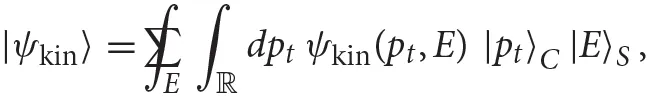
The form of δ(Ĉ_H) implies the decomposition of the physical Hilbert space into a direct sum of positive and negative frequency sectors ${{H}}_{\text{phys}}\simeq {{H}}_{+}\oplus {{H}}_{-}$ (see also [31, 104]). Acting with the projector δ(Ĉ_H) on an arbitrary kinematical state yields a physical state

where ψ_σ(E) are Newton-Wigner-type wave functions associated to the positive and negative frequency modes [90]⁶:

$\begin{array}{ll}{\psi }_{\sigma }(E)≔\frac{{\psi }_{\text{kin}}\left(p_{t,\sigma }(E),E\right)}{{(2|E|)}^{1/4}},& (16)\end{array}$

and we have defined the function $p_{t,\sigma }(E)≔-\sigma \sqrt{2|E|}$ and spectrum

$\begin{array}{l}{\sigma }_{SC}≔\text{Spec}({\widehat{H}}_S)\cap \text{Spec}(-{\widehat{H}}_C)\\ =\{E\in \text{Spec}({\widehat{H}}_S)|sE\le 0\}.& (17)\end{array}$

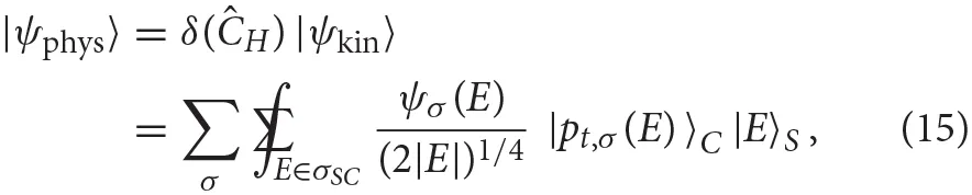
Physical states are normalized with respect to the physical inner product introduced in Equation (7)

which takes the usual form of non-relativistic quantum mechanics (σ-sector-wise), in line with the properties of Newton-Wigner-type wave functions. This observation will be crucial when discussing relativistic localization in section 6.

4. Covariant Clocks

4.1. Relational Dynamics With a Classical Covariant Clock

Exploiting the splitting of the degrees of freedom into clock C (our temporal reference system) and evolving system S, we now choose a clock function T on ${{P}}_C$ relative to which we describe the evolution of S in terms of relational observables, as discussed in section 2.1.

We could simply choose the phase space coordinate T = t as the clock function. It follows from Equation (2) that in the s = −1 case t runs “forward” on the positive frequency sector ${{C}}_{+}$ and “backward” on the negative frequency sector ${{C}}_{-}$ along the flow generated by C_H; for s = +1 the converse holds. Note that every point in ${{C}}_{+}\cap {{C}}_{-}$ corresponds to a static orbit of t (since p_t = 0 there), and t is therefore a maximally bad clock function on ${{C}}_{+}\cap {{C}}_{-}$. This leads to challenges in describing relational dynamics relative to t: inverse powers of p_t appear in the construction of relational observables encoding the evolution of system degrees of freedom relative to t when canonical pairs on ${{P}}_S$ are used [18, 23, 30, 31]⁷. One can solve this problem and obtain a well-defined relational dynamics by using affine (rather than canonical) pairs of evolving phase space coordinates on ${{P}}_S$ in the construction of relational observables [31], or in the quantum theory by carefully regularizing inverse powers of p_t [30].

However, in this article we shall sidestep these challenges and provide an arguably more elegant solution. We choose a different clock function according to the classical covariance condition: that it be canonically conjugate to H_C. This has the consequence of incorporating the pathology at p_t = 0 into the clock function (which will nevertheless be meaningfully quantized in section 4.2), and leads to relational observables which work independently of the choice of phase space coordinates on ${{P}}_S$. Solving {T, H_C} = 1, we find that a covariant clock function T must be of the form T = s t/p_t+g(p_t), where g(p_t) is an arbitrary function. Henceforth, we choose g(p_t) = 0 for simplicity, so that we have

$\begin{array}{ll}T=s\frac{t}{p_t}.& (19)\end{array}$

This clock function is well-defined everywhere, except on the line p_t = 0, where H_C is non-degenerate. It is clear that T runs “forward” everywhere on ${C}$ for both s = ±1, except on ${{C}}_{+}\cap {{C}}_{-}$.

The covariance condition, combined with our assumption that the clock does not interact with the system, implies that {T, C_H} = 1, which simplifies the form of the relational Dirac observables in Equation (4). For example, the relational observable corresponding to the question “what is the value of the system observable f_S when the clock T reads τ?” now takes the simple form [7, 21]

$\begin{array}{ll}{F}_{f_S,T}(\tau )\approx {\displaystyle \sum _{n=0}^{\infty }}\frac{{(\tau -T)}^n}{n!}{\{f_S,H_S\}}_n.& (20)\end{array}$

4.2. Covariant Quantum Time Observable for Quadratic Hamiltonians

One might try to construct a time operator in the quantum theory by directly quantizing the covariant clock function in Equation (19) on the clock Hilbert space ${{H}}_C\simeq L^2(ℝ)$ [86, 120, 121]. Choosing a symmetric ordering, this yields

$\begin{array}{ll}\widehat{T}=s\frac{1}{2}\left(\widehat{t}{\widehat{p}}_t^{-1}+{\widehat{p}}_t^{-1}\widehat{t}\right).& (21)\end{array}$

Here, ${\widehat{p}}_t^{-1}$ is defined in terms of a spectral decomposition such that $\widehat{T}|p_t=0\rangle$ is undefined, analogous to the classical case. While the operator $\widehat{T}$ is canonically conjugate to the clock Hamiltonian, $[\widehat{T},{Ĥ}_C]=i$, it is a symmetric operator that does not admit a self-adjoint extension [86, 88]. Since $\widehat{T}$ is not self-adjoint, its status as an observable seems a priori unclear⁸. This is a manifestation of Pauli's objection against the construction of time observables in quantum mechanics: For Ĥ_C bounded below, there does not exist a self-adjoint operator satisfying $[\widehat{T},{Ĥ}_C]=i$. Pauli's conclusion was that we are forced to treat time as a classical parameter, different to the way other observables (e.g., position and momentum) are treated [122].

However, it was later realized that by appealing to the more general notion of an observable offered by a POVM, a covariant time observable⁹ E_T can be constructed whose first moment corresponds to the operator $\widehat{T}$ [86, 87, 89]. Such a time observable is defined by a set of effect operator densities E_T(dt) ≥ 0 normalized as ${\int }_{ℝ}{E}_T(dt)=I_C$, and self-adjoint effect operators $E_T(X)≔{\int }_X{E}_T(dt)$ associated with the probability 〈ψ_C|E_T(X)|ψ_C〉 that a measurement of E_T yields an outcome t ∈ X ⊂ ℝ given that the clock was in the state $|{\psi }_C\rangle \in {{H}}_C$. In order to be a good time observable, it should satisfy the so-called covariance condition

$\begin{array}{ll}{E}_T(X+t)=U_C(t)E_T(X)U_C^{†}(t),& (23)\end{array}$

relative to the unitary group action $U_C(t)≔e^{-i{Ĥ}_{C}t}$ generated by the clock Hamiltonian. As we shall see shortly, this will give rise to a generalization of canonical conjugacy of the time observable and the clock Hamiltonian, and permit us to extend the approach to relational quantum dynamics based on covariant clock POVMs [7] to relativistic models. In particular, we obtain a valid quantum time observable despite the classical clock pathologies.

In the present case, such an observable can be constructed purely from the self-adjoint quantization of the clock Hamiltonian Ĥ_C and its eigenstates. The effect densities can be defined as a sum of “projections”

$\begin{array}{ll}{E}_T(dt)=\frac{1}{2\pi }{\displaystyle \sum _{\sigma }}dt|t,\sigma \rangle \langle t,\sigma |& (24)\end{array}$

onto the clock states corresponding to the clock reading t ∈ ℝ in the negative and positive frequency (i.e., positive and negative clock momentum) sector¹⁰

$\begin{array}{ll}|t,\sigma \rangle ≔{\displaystyle {\int }_{ℝ}}d{p}_t\sqrt{|p_t|}\theta (-\sigma p_t)e^{-its{p}_t^2/2}|p_t\rangle .& (25)\end{array}$

The covariance condition in Equation (23) is ensured by the fact that the clock states transform as

$\begin{array}{ll}|t+t^{\prime },\sigma \rangle =U_C\left(t\right)|t^{\prime },\sigma \rangle .& (26)\end{array}$

Note that the clock states are orthogonal to the pathological state |p_t = 0〉, so that the covariant time observable does not have support on it. The clock states are furthermore not mutually orthogonal:

$\begin{array}{ll}\langle t^{\prime },{\sigma }^{\prime }|t,\sigma \rangle ={\delta }_{\sigma {\sigma }^{\prime }}\left[\pi \delta (t-t^{\prime })-i\text{P}\frac{1}{t-t^{\prime }}\right],& (27)\end{array}$

where P denotes the Cauchy principal value. Hence E_T(dt) is not a true projector. Nevertheless, the following lemma demonstrates that the clock states |t, σ〉 form an over-complete basis for the σ-frequency sector of ${{H}}_C$, and in turn a properly normalized covariant time observable E_T on ${{H}}_{\text{kin}}$.

Lemma 1. The clock states |t, σ〉 defined in Equation (25) integrate to projectors $\theta (-\sigma {\widehat{p}}_t)$ onto the positive/negative frequency sector on ${{H}}_C$

$\begin{array}{ll}\frac{1}{2\pi }{\displaystyle {\int }_{ℝ}dt|t,\sigma \rangle \langle t,\sigma |=\theta (-\sigma {\widehat{p}}_t)}& (28)\end{array}$

and hence form a resolution of the identity as follows:

$\begin{array}{ll}{\displaystyle {\int }_{ℝ}E}(dt)=\frac{1}{2\pi }{\displaystyle \sum _{\sigma }{\displaystyle {\int }_{ℝ}d}}t|t,\sigma \rangle \langle t,\sigma |=I_C.& (29)\end{array}$

Proof: The proof is given in Supplementary Material. □

The n^th-moment operator of the time observable E_T is defined as

$\begin{array}{ll}{\widehat{T}}^{(n)}≔{\displaystyle {\int }_{ℝ}{E}_T}(dt)t^n=\frac{1}{2\pi }{\displaystyle \sum _{\sigma }{\displaystyle {\int }_{ℝ}d}}t{t}^n|t,\sigma \rangle \langle t,\sigma |.& (30)\end{array}$

While the effect operators of the clock POVM are self-adjoint, the moment operators for n ≥ 1 are not due to the non-orthogonality in Equation (27). Nevertheless, the latter are viable quantum observables with a valid probability interpretation in terms of the POVM; the only price to pay is that the different measurement outcomes t are not perfectly distinguishable.

With this definition, we find that the first-moment operator ${\widehat{T}}^{(1)}$ of E_T is in fact equal to the operator $\widehat{T}$ in Equation (21). This was previously noticed in Holevo [86] and Busch et al. [88] (for the s = +1 case). This provides a concrete interpretation of the time observable E_T in terms of the classical theory—the time operator ${\widehat{T}}^{(1)}$, namely the first moment of the time observable E_T, is the quantization of the classical clock function T in Equation (19).

Lemma 2. The operator $\widehat{T}$ and the first moment operator ${\widehat{T}}^{(1)}$ of the covariant time observable E_T are equal, $\widehat{T}\equiv {\widehat{T}}^{(1)}$.

Proof: The proof is given in Supplementary Material. □

Equation (30) demonstrates that the time operator $\widehat{T}$ automatically splits into a positive and negative frequency part, in contrast to $\widehat{t}$, the quantization of the phase space coordinate t.

Next, we find that while the clock states are not orthogonal, they are “almost” eigenstates of the covariant time operator $\widehat{T}$ on each σ-sector:

Lemma 3. The clock states |t, σ〉 defined in Equation (25) are not eigenstates of $\widehat{T}={\widehat{T}}^{(1)}$. However, for all $|\psi \rangle \in {D}(\widehat{T})$, where ${D}(\widehat{T})$ is the domain of $\widehat{T}$, they satisfy:

$\begin{array}{l}\langle \psi |\widehat{T}|t,\sigma \rangle =t\langle \psi |t,\sigma \rangle ,\forall t\in ℝ,\sigma =\pm 1.\end{array}$

Proof: The proof is given in Supplementary Material. □

This leads to a another result, which underscores why the covariance condition Equation (23) can be regarded as yielding a generalization of canonical conjugacy:

Lemma 4. The nth-moment operator defined in Equation (30) satisfies $[{\widehat{T}}^{(n)},{Ĥ}_C]=in{\widehat{T}}^{(n-1)}$. Furthermore, $\forall |\psi \rangle \in {D}({\widehat{T}}^n)$ we have ${\widehat{T}}^{(n)}|\psi \rangle ={\widehat{T}}^n|\psi \rangle$.

Proof: The proof is given in Supplementary Material. □

We emphasize that the second statement of Lemma 4 does not hold on all of ${{H}}_C$.

The effect density does not commute with the clock Hamiltonian, [E_T(dt), Ĥ_C] ≠ 0, which implies the time indicated by the clock (i.e., a measurement outcome of E_T) and the clock energy cannot be determined simultaneously. However, importantly, the following lemma shows that the clock reading and the frequency sector, i.e., the value of σ can be simultaneously determined.

Lemma 5. The effect density E_T(dt) of the covariant clock POVM and the projectors onto the σ-sectors commute: $[E_T(dt),\theta (-\sigma {\widehat{p}}_t)]=0$.

Proof: The proof is given in Supplementary Material. □

Corollary 1. Since the effect density integrates to the effect and moment operators, this entails that $[E_T(X),\theta (-\sigma {\widehat{p}}_t)]=[{\widehat{T}}^{(n)},\theta (-\sigma {\widehat{p}}_t)]=0$, for all X ⊂ ℝ and n ∈ ℕ.

The significance of this lemma and corollary is that they permit us to condition on the time indicated by the clock and the frequency sector simultaneously. This will become crucial when defining the quantum reduction maps below that take us from the physical Hilbert space to the relational Schrödinger and Heisenberg pictures which exist for each σ-sector. This lemma is thus an important for extending the quantum reduction procedures of Höhn et al. [7] to the class of models considered here.

5. The Trinity of Relational Quantum Dynamics: Quadratic Clock Hamiltonians

Having introduced the clock-neutral structure of the classical and quantum theories in section 2, a natural partitioning of the kinematical degrees of freedom into a clock C and system S in section 3, and a covariant time observable E_T in section 4, we are now able to construct a relational quantum dynamics, describing how S evolves relative to C.

As noted in the introduction, we showed in Höhn et al. [7] that three formulations of relational quantum dynamics, namely (i) quantum relational Dirac observables, (ii) the relational Schrödinger picture of the Page-Wootters formalism, and (iii) the relational Heisenberg picture obtained through quantum deparametrization, are equivalent for models described by the Hamiltonian constraint in Equation (9) when the clock Hamiltonian has a continuous, non-degenerate spectrum; the three formulations form a trinity of relational quantum dynamics. Here we demonstrate that this equivalence extends to constraints of the form in Equation (13), involving the doubly degenerate clock Hamiltonian¹¹.

Thanks to the direct sum structure of the physical Hilbert space ${{H}}_{\text{phys}}={{H}}_{+}\oplus {{H}}_{-}$ and the separation of the clock moment operators (Equation 30), into non-degenerate positive and negative frequency sectors, all the technical results needed for establishing the equivalence in Höhn et al. [7] will hold per σ-sector for the present class of models. We will thus state some of the following results without proofs, referring the reader as approriate to the proofs of the corresponding results in Höhn et al. [7], which apply here per σ-sector. In particular, Corollary 1 implies that we are permitted to simultaneously condition on the clock reading and the frequency sector.

Lastly, we also provide a discussion of the relational quantum dynamics obtained through reduced phase space quantization. In this case, one deparametrizes the model classically relative to the clock function T, which amounts to a classical symmetry reduction. While the relational quantum dynamics thus obtained yields a relational Heisenberg picture resembling dynamics (iii) of the trinity, it is not always equivalent and thus not necessarily part of the trinity. For this reason, we have moved the exposition of reduced phase space quantization to Supplementary Material. It is however useful for understanding why the quantum symmetry reduction explained below is the quantum analog of classical phase space reduction through deparametrization. We emphasize that symmetry reduction and quantization do not commute in general [7, 124–129]. A related discussion for relativistic constraints can also be found in Kaminski et al. [29].

To aid the reader, we summarize the various Hilbert spaces appearing in the construction of the trinity in Table 2.

TABLE 2

Table 2. Summary of different Hilbert spaces.

5.1. The Three Faces of the Trinity

5.1.1. Dynamics (i): Quantum Relational Dirac Observables

We now quantize the relational Dirac observables in Equation (20), substantiating the discussion of relational quantum dynamics in the clock-neutral picture in section 2.2 for Hamiltonian constraints of the form Equation (13). Quantization of relational Dirac observables has been studied when the quantization of the classical time function T results in a self-adjoint time operator $\widehat{T}$ (see [4, 7, 11–20, 27–31, 35–38, 116] and references therein); however, when $\widehat{T}$ fails to be self-adjoint, such as in Equation (21), a more general quantization procedure is needed.

Such a procedure was introduced in Höhn et al. [7] based upon the quantization of Equation (20) using covariant time observables. Applying this procedure to the present class of models described by quadratic clock Hamiltonians, we quantize the relational Dirac observables in Equation (20) using the nth-moment operators defined in Equation (30):

$\begin{array}{l}{\widehat{F}}_{f_S,T}(\tau )≔{\displaystyle {\int }_{ℝ}}{E}_T(dt)\otimes {\displaystyle \sum _{n=0}^{\infty }}\frac{i^n}{n!}{(t-\tau )}^n[{\widehat{f}}_S,{\widehat{H}}_S{]}_n\\ ={\displaystyle \sum _{\sigma }}{\displaystyle {\int }_{ℝ}}\frac{dt}{2\pi }{U}_{CS}(t)(|\tau ,\sigma \rangle \langle \tau ,\sigma |\otimes {\widehat{f}}_S)U_{CS}^{†}(t)\\ =:{\displaystyle \sum _{\sigma }}{G}(|\tau ,\sigma \rangle \langle \tau ,\sigma |\otimes {\widehat{f}}_S),& (31)\end{array}$

where ${[{\widehat{f}}_S,{Ĥ}_S]}_n≔[{[{\widehat{f}}_S,{Ĥ}_S]}_{n-1},{Ĥ}_S]$ is the nth-order nested commutator with the convention ${[{\widehat{f}}_S,{Ĥ}_S]}_0≔{\widehat{f}}_S$, U_CS(t) ≔ exp(−i t Ĉ_H), and the second line follows upon a change of integration variable and invoking the covariance condition in Equation (26). The relational Dirac observable ${\widehat{F}}_{f_S,T}(\tau )$ is thus revealed to be an incoherent average over the one-parameter non-compact gauge group G generated by the constraint operator Ĉ_H of the kinematical operator $|\tau ,\sigma \rangle \langle \tau ,\sigma |\otimes {\widehat{f}}_S$ paired with the projector onto the clock reading τ and the σ-frequency sector. Such a group averaging is known as the G-twirl operation and we denote it ${G}$ as in the last line of Equation (31). G-twirl operations have previously been mostly studied in the context of spatial quantum reference frames, e.g., see [130–132], but have also appeared in some constructions of quantum Dirac observables (e.g., see [7, 11, 37, 38, 106])¹². As discussed in Höhn et al. [7], this G-twirl constitutes the quantum analog of a gauge-invariant extension of a gauge-fixed quantity.

The relational Dirac observables ${\widehat{F}}_{f_S,T}(\tau )$ in Equation (31) constitute a one-parameter family of strong Dirac observables on ${{H}}_{\text{phys}}$ (Theorem 1 of [7] whose proof applies here in each σ-sector):

$\begin{array}{ll}\left[{\widehat{F}}_{f_S,T}(\tau ),{\widehat{C}}_H\right]=0,\forall \tau \in ℝ.& (32)\end{array}$

We thus obtain a gauge-invariant relational quantum dynamics by letting the evolution parameter τ in the physical expectation values ${\langle {\psi }_{\text{phys}}|{\widehat{F}}_{f_S,T}(\tau )|{\psi }_{\text{phys}}\rangle }_{\text{phys}}$ run.

The decomposition of ${\widehat{F}}_{f_S,T}(\tau )$ in Equation (31) into positive and negative frequency sectors gives rise to a reducible representation of the Dirac observable algebra on the physical Hilbert space. More precisely, relational Dirac observables are superselected across the σ-frequency sectors, and the σ-sum in Equation (31) should thus be understood as a direct sum. To see this, consider the operator $\widehat{Q}≔\theta (-{\widehat{p}}_t)-\theta ({\widehat{p}}_t)$, where we recall that $\theta (-\sigma {\widehat{p}}_t)$ is a projector onto the corresponding σ-sector. By construction $[\widehat{Q},{Ĉ}_H]=0$, which means that $\widehat{Q}$ is a strong Dirac observable. Its eigenspaces, with eigenvalues +1 and −1, correspond to the positive and negative frequency sector subspaces ${{H}}_{+}$ and ${{H}}_{-}$. Furthermore, $\widehat{Q}$ commutes with any relational Dirac observable F_fS,T(τ) in Equation (31) on account of Lemma 5, which implies that Q and any self-adjoint F_fS,T(τ) can be diagonalized in the same eigenbasis. This in turn implies the following superselection rule

$\begin{array}{ll}{\widehat{F}}_{f_S,T}(\tau )={\widehat{F}}_{f_S,T}^{+}(\tau )\oplus {\widehat{F}}_{f_S,T}^{-}(\tau ),& (33)\end{array}$

where ${\widehat{F}}_{f_S,T}^{\sigma }(\tau )≔{G}\left(|\tau ,\sigma \rangle \langle \tau ,\sigma |\otimes {\widehat{f}}_S\right)\in {L}\left({{H}}_{\sigma }\right)$¹³.

While there do exist states in the physical Hilbert space that exhibit coherence across the σ-frequency sectors, for example |ψ_phys〉 ~ |ψ₊〉 + |ψ₋〉, where $|{\psi }_{\sigma }\rangle \in {{H}}_{\sigma }$, such coherence is not physically accessible because it does not affect the expectation value of any relational Dirac observable on account of the decomposition in Equation (33). In other words, superpositions and classical mixtures across the σ-frequency sectors are indistinguishable. Hence, superpositions of physical states across σ-sectors are mixed states and the pure physical states are those of either ${{H}}_{+}$ or ${{H}}_{-}$ (see also [103, 105] for a discussion on superselection in group averaging).

For example, this superselection rule manifests as a superselection across positive and negative frequency modes in the case of the relativistic particle and across expanding and contracting solutions in the case of the FLRW model with a massless scalar field in Table 1 [31]. On account of the reducibility of the representation, one usually restricts to one frequency sector (e.g., see [113, 114, 116, 133]). One might conjecture that the analogous superselection rule in a quantum field theory would manifest as a superselection rule between matter and anti-matter sectors.

Superselection rules induced by the G-twirl are often interpreted as arising from the lack of knowledge about a reference frame, and that if an appropriate reference frame is used the superselection rule can be lifted [130]. This interpretation seems unsuitable here. Firstly, lifting the superselection rule would entail undoing the group averaging, in violation of gauge invariance. Secondly, such an interpretation is usually tied to an average over a given group action which parametrizes one's ignorance about relative reference frame orientations. By contrast, the origin of the superselection of Dirac observables here is not the group generated by the constraint, but is a consequence of a property of the constraint, i.e., the group generator. Indeed, the superselection rule above originates in the factorizability of the constraint and the ensuing decomposition of the projector onto the constraint (Equation 14). Both these properties rely on the absence of a $\widehat{t}$-dependent term in the constraint Equation (13); if such a term is introduced, one generally finds [Ĉ₊, Ĉ₋] ≠ 0, where the Ĉ_σ are the quantization of the classical factors, but we emphasize that Ĉ_H ≠ s Ĉ₊Ĉ₋ in that case. While such a modified constraint may generate the same group¹⁴, no superselection rule across the σ-sectors would arise. The above superselection rule can thus not be associated with the lack of a shared physical reference frame. This resonates with the interpretation of the physical Hilbert space as a clock-neutral, i.e., temporal-reference-frame-neutral structure (see section 2.2).

Consider now the projector Π_σSC = θ(−s Ĥ_S) from ${{H}}_S$ to its subspace spanned by all system energy eigenstates |E〉_S with E ∈ σ_SC; that is, those permitted upon solving the constraint Equation (13). We shall henceforth denote this system Hilbert subspace ${{H}}_S^{\text{phys}}≔{\Pi }_{{\sigma }_{SC}}({{H}}_S)$ and call it the physical system Hilbert space. We will obtain two copies of the physical system Hilbert space, one for each frequency sector. In analogy to the classical case, we introduce the quantum weak equality between operators, signifying that they are equal on the “quantum constraint surface” ${{H}}_{\text{phys}}$:

$\begin{array}{l}{Ô}_1\approx {Ô}_2\\ \iff {\widehat{O}}_1|{\psi }_{\text{phys}}\rangle ={\widehat{O}}_2|{\psi }_{\text{phys}}\rangle ,\forall |{\psi }_{\text{phys}}\rangle \in {{H}}_{\text{phys}}.& (34)\end{array}$

It follows from Lemma 1 of [7], whose proof applies here per σ-sector, that

$\begin{array}{ll}{\widehat{F}}_{f_S,T}(\tau )\approx {\widehat{F}}_{{\Pi }_{{\sigma }_{SC}}{f}_S{\Pi }_{{\sigma }_{SC}},T}(\tau ),& (35)\end{array}$

are weakly equal relational Dirac observables. Hence, the relational Dirac observables in Equation (31) form weak equivalence classes on ${{H}}_{\text{phys}}$, where ${\widehat{F}}_{f_S,T}(\tau )~{\widehat{F}}_{g_S,T}(\tau )$ if ${\Pi }_{{\sigma }_{SC}}{\widehat{f}}_S{\Pi }_{{\sigma }_{SC}}={\Pi }_{{\sigma }_{SC}}{ĝ}_S{\Pi }_{{\sigma }_{SC}}$. These weak equivalence classes are labeled by what we shall denote

$\begin{array}{ll}{\widehat{f}}_S^{\text{phys}}≔{\Pi }_{{\sigma }_{SC}}{\widehat{f}}_S{\Pi }_{{\sigma }_{SC}}\in {L}\left({{H}}_S^{\text{phys}}\right),& (36)\end{array}$

for arbitrary ${\widehat{f}}_S\in {L}({{H}}_S)$, where ${L}$ denotes the set of linear operators. For later use, we note that the algebras of the physical system observables ${\widehat{f}}_S^{\text{phys}}$ on ${{H}}_S^{\text{phys}}$ and the ${\widehat{F}}_{f_S^{\text{phys}},T}(\tau )$ on ${{H}}_{\text{phys}}$ are weakly homomorphic with respect to addition, multiplication and commutator relations. More precisely,

$\begin{array}{l}{\widehat{F}}_{f_S^{\text{phys}}+g_S^{\text{phys}}·h_S^{\text{phys}},T}(\tau )\approx {\widehat{F}}_{f_S^{\text{phys}},T}(\tau )\\ +{\widehat{F}}_{g_S^{\text{phys}},T}(\tau )·{\widehat{F}}_{h_S^{\text{phys}},T}(\tau )\end{array}$

$\forall f_S,g_S,h_S\in {L}({{H}}_S)$. This is a consequence of Theorem 2 of Höhn et al. [7] (whose proof again applies here per σ-sector). Together with Höhn et al. [7], this translates the weak classical algebra homomorphism defined through relational observables in Dittrich [21] into the quantum theory.

5.1.2. Dynamics (ii): The Page-Wootters Formalism

Suppose we are given a quantum Hamiltonian constraint Equation (5) which splits into a clock and system contribution as in Equation (9), but for the moment not necessarily assuming it to be of the quadratic form in Equation (13). Suppose further we are given some (kinematical) time observable on the clock Hilbert space, which need not necessarily be a clock POVM which is covariant with respect to the group generated by the clock Hamiltonian, but is taken to define the clock reading. Page and Wootters [39, 40, 134, 135] proposed to extract a relational quantum dynamics between the clock and system from physical states in terms of conditional probabilities: what is the probability of an observable ${\widehat{f}}_S$ associated with the system S giving a particular outcome f, if the measurement of the clock's time observable yields the time τ? If e_C(τ) and e_fS(f) are the projectors onto the clock reading τ and the system observable ${\widehat{f}}_S$ taking the value f, this conditional probability is postulated in the form

$\begin{array}{l}\text{Prob}(f\text{when }\tau )=\frac{\text{Prob}(f\text{and }\tau )}{\text{Prob}(\tau )}\\ =\frac{\langle {\psi }_{\text{phys}}|e_C(\tau )\otimes e_{f_S}(f){|{\psi }_{\text{phys}}\rangle }_{\text{kin}}}{\langle {\psi }_{\text{phys}}|e_C(\tau )\otimes I_S{|{\psi }_{\text{phys}}\rangle }_{\text{kin}}}.& (37)\end{array}$

This expression appears at first glimpse to be in violation of the constraints, as it acts with operators on physical states that are not Dirac observables; this is the basis of Kuchař's criticism (b) that the conditional probabilities of the Page-Wootters formalism are incompatible with the constraints [1]. However, for a class of models we have shown in Höhn et al. [7] that the expression Equation (37) is a quantum analog of a gauge-fixed expression of a manifestly gauge-invariant quantity and thus consistent with the constraint. In this section we extend this result to relativistic settings.

Here we shall expand the Page-Wootters formalism to the more general class of Hamiltonian constraints of the form Equation (13) exploiting the covariant clock POVM E_T of section 4.2¹⁵. On the one hand, this will permit us to prove full equivalence of the so-obtained relational quantum dynamics with the manifestly gauge-invariant formulation in terms of relational Dirac observables on ${{H}}_{\text{phys}}$ of Dynamics (i). As an aside, this will also resolve the normalization issue of physical states appearing in Diaz et al. [50], where the kinematical rather than physical inner product was used to normalize physical states, thus yielding a divergence (when used for equal mass states). On the other hand, the covariant clock POVM will allow us, in section 6, to address the observation by Kuchař [1] that using the Minkowski time observable leads to incorrect localization probabilities for relativistic particles in the Page-Wootters formalism.

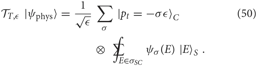
The Page-Wootters formalism produces the system state at clock time τ by conditioning physical states on the clock reading τ [39, 40, 134, 135]. Henceforth focusing on the class of models defined by the constraint in Equation (13) and the covariant clock POVM of section 4.2, and given the reducible representation of ${{H}}_{\text{phys}}$, we may additionally condition on the frequency sector thanks to Lemma 5. In extension of Höhn et al. [7], we may use this conditioning to define two reduction maps ${{R}}_{\text{S}}^{\sigma }(\tau ):{{H}}_{\text{phys}}\to {{H}}_{S,\sigma }^{\text{phys}}$, one per σ-frequency sector,

$\begin{array}{ll}{{R}}_S^{\sigma }(\tau )≔\langle \tau ,\sigma |\otimes I_S,& (38)\end{array}$

where ${{H}}_{S,\sigma }^{\text{phys}}$ is a copy of ${{H}}_S^{\text{phys}}={\Pi }_{{\sigma }_{SC}}({{H}}_S)$, i.e., the subspace of the system Hilbert space permitted upon solving the constraint, corresponding to the σ-frequency sector. As will become clear shortly, the label S on the reduction map stands for “Schrödinger picture” and to distinguish it from the italic S which stands for the system, we henceforth write it in bold face. Due to the decomposition ${{H}}_{\text{phys}}={{H}}_{+}\oplus {{H}}_{-}$, we equip the two copies ${{H}}_{S,\sigma }^{\text{phys}}$ with the frequency label σ in order to remind ourselves which reduced theory corresponds to which positive or negative frequency mode.

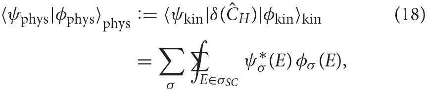
The reduced states (whose normalization factor $1/\sqrt{2}$ will be explained later),

where ψ_σ(E) is the Newton-Wigner type wave function defined in Equation (16), satisfy the Schrödinger equation with respect to Ĥ_S:

$\begin{array}{ll}i\frac{d}{d\tau }|{\psi }_S^{\sigma }(\tau )\rangle ={\widehat{H}}_S|{\psi }_S^{\sigma }(\tau )\rangle .& (40)\end{array}$

We interpret this as the dynamics of S relative to the temporal reference frame C. In particular, this Schrödinger equation looks the same for both the positive and negative frequency sectors because the time defined by the covariant clock POVM E_T runs forward in both sectors. This is clear from Equation (26) and is the quantum analog of the earlier classical observation that the clock function T runs “forward” on both frequency sectors ${{C}}_{+}$ and ${{C}}_{-}$ (in contrast to t)¹⁶.

Thanks to Equation (29), the decomposition of the physical states into positive and negative frequency modes, Equation (15) can also be written as follows:

$\begin{array}{ll}|{\psi }_{\text{phys}}\rangle =\frac{1}{2\sqrt{2}\pi }{\displaystyle \sum _{\sigma }{\displaystyle {\int }_{ℝ}dt|t,\sigma \rangle |{\psi }_S^{\sigma }(t)\rangle .}}& (41)\end{array}$

Together with Lemma 1, this implies that the σ-sector left inverse ${{H}}_{S,\sigma }^{\text{phys}}\to {{H}}_{\sigma }$ of the reduction map defined in Equation (38) is given by

$\begin{array}{ll}\begin{array}{c}{({{R}}_S^{\sigma }(\tau ))}^{-1}=\frac{1}{2\pi }{\displaystyle {\int }_{ℝ}dt|t,\sigma \rangle \otimes U_S(t-\tau )}\\ =\delta ({\widehat{C}}_H)(|\tau ,\sigma \rangle \otimes I_S),\end{array}& (42)\end{array}$

where U_S(t) = exp(−i Ĥ_S t), so that

$\begin{array}{l}{({{R}}_{\text{S}}^{\sigma }(\tau ))}^{-1}{{R}}_{\text{S}}^{\sigma }(\tau )=\delta ({\widehat{C}}_H)(|\tau ,\sigma \rangle \langle \tau ,\sigma |\otimes I_S)\\ \approx \theta (-\sigma {\widehat{p}}_t)\otimes I_S,& (43)\end{array}$

where ≈ is the quantum weak equality, and thus

$\begin{array}{ll}{\displaystyle \sum _{\sigma }}{({{R}}_{\text{S}}^{\sigma }(\tau ))}^{-1}{{R}}_{\text{S}}^{\sigma }(\tau )\approx I_{\text{phys}}.& (44)\end{array}$

Conversely, we can write the identity on ${{H}}_{S,\sigma }^{\text{phys}}$ in the form

$\begin{array}{l}{{R}}_{\text{S}}^{\sigma }(\tau ){({{R}}_{\text{S}}^{\sigma }(\tau ))}^{-1}=\langle \tau ,\sigma |\delta ({\widehat{C}}_H)|\tau ,\sigma \rangle \\ ={\Pi }_{{\sigma }_{SC}}.\end{array}$

The identity in the second line can be checked with the help of Equation (27) (and also follows from the proof of Theorem 2 in [7]). A summary of these maps can be found in Figure 2.

FIGURE 2

Figure 2. A summary of the Page-Wootters reduction maps and their inverses. The analogous state of affairs holds for the quantum symmetry reduction maps and their inverses.

Using these reduction maps and their inverses, we can define an encoding operation ${{E}}_{\text{S}}^{\tau ,\sigma }:{L}\left({{H}}_{S,\sigma }^{\text{phys}}\right)\to {L}({{H}}_{\sigma })$, mapping the observables in Equation (36), acting on the physical system Hilbert space ${{H}}_{S,\sigma }^{\text{phys}}$, into Dirac observables on the σ-sector of ${{H}}_{\text{phys}}$:

$\begin{array}{l}{{E}}_{\text{S}}^{\tau ,\sigma }\left({\widehat{f}}_S^{\text{phys}}\right)≔{({{R}}_{\text{S}}^{\sigma }(\tau ))}^{-1}{\widehat{f}}_S^{\text{phys}}{{R}}_{\text{S}}^{\sigma }(\tau )\\ =\delta ({\widehat{C}}_H)(|\tau ,\sigma \rangle \langle \tau ,\sigma |\otimes {\widehat{f}}_S^{\text{phys}}).& (45)\end{array}$

These encoded observables turn out to be the σ-sector part of the relational Dirac observables in Equation (31), as articulated in the following theorem.

Theorem 1. Let ${\widehat{f}}_S\in {L}({{H}}_S)$. The quantum relational Dirac observable ${\widehat{F}}_{f_S,T}(\tau )$ acting on ${{H}}_{\text{phys}}$, Equation (31), reduces under ${{R}}_{\text{S}}^{\sigma }(\tau )$ to the corresponding projected observable on ${{H}}_{S,\sigma }^{\text{phys}}$,

$\begin{array}{l}{{R}}_{\text{S}}^{\sigma }(\tau ){\widehat{F}}_{f_S,T}(\tau ){({{R}}_{\text{S}}^{\sigma }(\tau ))}^{-1}={\Pi }_{{\sigma }_{SC}}{\widehat{f}}_S{\Pi }_{{\sigma }_{SC}}\equiv {\widehat{f}}_S^{\text{phys}}.\end{array}$

Conversely, let ${\widehat{f}}_S^{\text{phys}}\in {L}\left({{H}}_{S,\sigma }^{\text{phys}}\right)$. The encoding operation in Equation (45) of system observables coincides on the physical Hilbert space ${{H}}_{\text{phys}}$ with the quantum relational Dirac observables in Equation (31) projected into the σ-sector:

$\begin{array}{ll}{{E}}_{\text{S}}^{\tau ,\sigma }\left({\widehat{f}}_S^{\text{phys}}\right)\approx {\widehat{F}}_{f_S^{\text{phys}},T}^{\sigma }(\tau ),& (46)\end{array}$

where ${\widehat{F}}_{f_S^{\text{phys}},T}^{\sigma }(\tau )={\widehat{F}}_{f_S^{\text{phys}},T}(\tau )(\theta (-\sigma {\widehat{p}}_t)\otimes I_S)$—c.f. Equation (33).

Proof: The proof of Theorem 3 in Höhn et al. [7] applies here per σ-sector. □

Note that the relational Dirac observables ${\widehat{F}}_{f_S,T}(\tau )$ commute with the projectors $\theta (-\sigma {\widehat{p}}_t)$ due to the reducible representation in Equation (31).

Apart from providing the σ-sector-wise dictionary between the observables on the physical Hilbert space and the physical system Hilbert space, Theorem 1, in conjunction with the weak equivalence in Equation (35), also implies an equivalence between the full sets of relational Dirac observables ${\widehat{F}}_{f_S^{\text{phys}},T}^{\sigma }(\tau )$ on ${{H}}_{\sigma }$ and system observables on ${{H}}_{S,\sigma }^{\text{phys}}$.

Crucially, the expectation values of the relational Dirac observables Equation (31) in the physical inner product Equation (18) coincide, σ-sector-wise, with the expectation values of the physically permitted system observables ${\widehat{f}}_S^{\text{phys}}$ in the states solving the Schrödinger equation Equation (40) on ${{H}}_{S,\sigma }^{\text{phys}}$.

Theorem 2. Let ${\widehat{f}}_S\in {L}({{H}}_S)$, and denote its associated operator on ${{H}}_S^{\text{phys}}$ by ${\widehat{f}}_S^{\text{phys}}={\Pi }_{{\sigma }_{SC}}{\widehat{f}}_S{\Pi }_{{\sigma }_{SC}}$. Then

$\langle {\psi }_{\text{phys}}|{\widehat{F}}_{f_S,T}^{\sigma }\left(\tau \right){|{\varphi }_{\text{phys}}\rangle }_{\text{phys}}=\frac{1}{2}\langle {\psi }_S^{\sigma }\left(\tau \right)|{\widehat{f}}_S^{\text{phys}}|{\varphi }_S^{\sigma }\left(\tau \right)\rangle ,$

where $|{\psi }_S^{\sigma }(\tau )\rangle =\sqrt{2}{{R}}_{\text{S}}^{\sigma }(\tau )|{\psi }_{\text{phys}}\rangle$ as in Equation (39). Hence,

$\langle {\psi }_{\text{phys}}|{\widehat{F}}_{f_S,T}\left(\tau \right){|{\varphi }_{\text{phys}}\rangle }_{\text{phys}}=\frac{1}{2}{\displaystyle \sum _{\sigma }\langle {\psi }_S^{\sigma }\left(\tau \right)|{\widehat{f}}_S^{\text{phys}}|{\varphi }_S^{\sigma }\left(\tau \right)\rangle },$

Proof: The proof of Theorem 4 in Höhn et al. [7] applies here per σ-sector. □

Hence, the expectation values in the relational Schrödinger picture (i.e., the Page-Wootters formalism) are equivalent to the gauge-invariant ones of the corresponding relational Dirac observables on ${{H}}_{\text{phys}}$. Accordingly, equations, such as Equation (37) (adapted to σ-sectors) are not in violation of the constraint as claimed by Kuchař [1].

This immediately implies that the reduction maps ${{R}}_{\text{S}}^{\sigma }(\tau )$ preserve inner products per σ-sector as follows.

Corollary 2. Setting ${\widehat{f}}_S={\Pi }_{{\sigma }_{SC}}$ in Theorem 2 yields

$\langle {\psi }_{\text{phys}}|\theta (-\sigma {\widehat{p}}_t)\otimes I_S{|{\varphi }_{\text{phys}}\rangle }_{\text{phys}}=\frac{1}{2}\langle {\psi }_S^{\sigma }(\tau )|{\varphi }_S^{\sigma }(\tau )\rangle ,$

where $|{\psi }_S^{\sigma }(\tau )\rangle =\sqrt{2}{{R}}_{\text{S}}^{\sigma }(\tau )|{\psi }_{\text{phys}}\rangle$. Hence,

$\begin{array}{ll}\begin{array}{l}{\langle {\psi }_{\text{phys}}|{\varphi }_{\text{phys}}\rangle }_{\text{phys}}=\frac{1}{2}{\displaystyle \sum _{\sigma }\langle {\psi }_S^{\sigma }\left(\tau \right)|{\varphi }_S^{\sigma }\left(\tau \right)\rangle }\hfill \\ ={\displaystyle \sum _{\sigma }\langle {\psi }_{\text{phys}}|\left(|\tau ,\sigma \rangle \langle \tau ,\sigma |\otimes I_S\right){|{\varphi }_{\text{phys}}\rangle }_{\text{kin}}}.\hfill \end{array}& (47)\end{array}$

The reason for introducing the normalization factor $1/\sqrt{2}$ in Equation (39) is now clear: it permits us to work with normalized states $\langle {\psi }_S^{\sigma }(\tau )|{\psi }_S^{\sigma }(\tau )\rangle =1={\langle {\psi }_{\text{phys}}|{\psi }_{\text{phys}}\rangle }_{\text{phys}}$ in each reduced σ-sector and in the physical Hilbert space simultaneously.

The above results show:

(1) Applying the Page-Wootters reduction map ${{R}}_{\text{S}}^{\sigma }(\tau )$ to the physical Hilbert space ${{H}}_{\text{phys}}$ yields a relational Schrödinger picture with respect to the clock C on the physical system Hilbert space ${{H}}_{S,\sigma }^{\text{phys}}$ corresponding to the σ-frequency sector.

(2) σ-sector wise, the relational quantum dynamics encoded in the relational Dirac observables on the physical Hilbert space is equivalent to the dynamics in the relational Schrödinger picture on the physical system Hilbert space of the Page-Wootters formalism.

(3) Given the invertibility of the reduction map, Theorem 2 formally shows that if ${\widehat{f}}_S^{\text{phys}}$ is self-adjoint on ${{H}}_{S,\sigma }^{\text{phys}}$, then so is ${\widehat{F}}_{f_S,T}^{\sigma }(\tau )$ on ${{H}}_{\sigma }$.

We note that the expression in the second line of Equation (47) also defines an inner product on the space of solutions to the Wheeler-DeWitt-type constraint Equation (13), which is equivalent to the physical inner product in Equation (18) obtained through group averaging. These two inner products thus define the same physical Hilbert space ${{H}}_{\text{phys}}$. The expression in the second line of Equation (47) is the adaptation of the Page-Wootters inner product introduced in Smith and Ahmadi [44] to the reducible representation of the physical Hilbert space associated to Hamiltonian constraints with quadratic clock Hamiltonians.

5.1.3. Dynamics (iii): Quantum Deparametrization

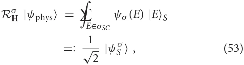
Classically, one can perform a symmetry reduction of the clock-neutral constraint surface by gauge-fixing the flow of the constraint. In this case, this yields two copies of a gauge-fixed reduced phase space, one for each frequency sector, each equipped with a standard Hamiltonian dynamics, hence yielding a deparametrized theory (see Supplementary Material). In contrast to the classical constraint surface, the “quantum constraint surface” ${{H}}_{\text{phys}}$ is automatically gauge-invariant since the exponentiation of the symmetry generator Ĉ_H acts trivially on all physical states and Dirac observables. Hence, there is no more gauge-fixing in the quantum theory after solving the constraint. Nevertheless, following Höhn and Vanrietvelde [30], Höhn [31], and Höhn et al. [7], we now demonstrate the quantum analog of the classical symmetry reduction procedure for the class of models considered in this article. As such it is the quantum analog of deparametrization, which we henceforth refer to as quantum deparametrization. This quantum symmetry reduction maps the clock-neutral Dirac quantization to a relational Heisenberg picture relative to clock observable E_T, and involves the following two steps.

1. Constraint trivialization: A transformation of the constraint such that it only acts on the chosen reference system (here clock C), fixing its degrees of freedom. The classical analog is a canonical transformation which turns the constraint into a momentum variable and separates gauge-variant from gauge-invariant degrees of freedom [7, 71].

2. Condition on classical gauge fixing conditions: A “projection” which removes the now redundant reference frame degrees of freedom¹⁷.

We begin by defining the constraint trivialization map ${{T}}_{T,ϵ}:{{H}}_{\text{phys}}\to {{T}}_{T,ϵ}({{H}}_{\text{phys}})$ relative to the covariant time observable E_T. This map will transform the physical Hilbert space into a new Hilbert space, while preserving inner products and algebraic properties of observables

$\begin{array}{l}{{T}}_{T,ϵ}≔{\displaystyle \sum _{n=0}^{\infty }}\frac{i^n}{n!}{\widehat{T}}^{(n)}\otimes {\left({\widehat{H}}_S+s\frac{{ϵ}^2}{2}\right)}^n\\ =\frac{1}{2\pi }{\displaystyle \sum _{\sigma }{\displaystyle {\int }_{ℝ}dt|t,\sigma \rangle }\langle t,\sigma |\otimes e^{it\left({\widehat{H}}_S+s{\in }^2/2\right)}}.& (48)\end{array}$

In analogy to Höhn and Vanrietvelde [30], Höhn [31], and Höhn et al. [7], we introduce an arbitrary positive parameter ϵ > 0 so that the map becomes invertible. Note that $s{ϵ}^2/2\in \mathrm{\text{Spec}}({Ĥ}_C)$.

Lemma 6. The left inverse of the trivialization ${{T}}_{T,ϵ}$ is given by

${{T}}_{T,\in }^{-1}=\frac{1}{2\pi }{\displaystyle \sum _{\sigma }{\displaystyle {\int }_{ℝ}dt|t,\sigma \rangle }\langle t,\sigma |\otimes e^{it\left({\widehat{H}}_S+s{\in }^2/2\right)}},$

so that, for any ϵ > 0, ${{T}}_{T,ϵ}^{-1}:{{T}}_{T,ϵ}({{H}}_{\text{phys}})\to {{H}}_{\text{phys}}$ and

$\begin{array}{l}{{T}}_{T,ϵ}^{-1}○{{T}}_{T,ϵ}\approx I_{\text{phys}}.\end{array}$

Proof: The proof of Lemma 2 in Höhn et al. [7] applies here σ-sector wise. □

The main property of the trivialization map is summarized in the following lemma.

Lemma 7. The map ${{T}}_{T,ϵ}$ trivializes the constraint in Equation (13) to the clock degrees of freedom

$\begin{array}{ll}{{T}}_{T,ϵ}{\widehat{C}}_H{{T}}_{T,ϵ}^{-1}\stackrel{*}{\approx }\frac{s}{2}({\widehat{p}}_t^2-{ϵ}^2)\otimes I_S,& (49)\end{array}$

where $\stackrel{*}{\approx }$ is the quantum weak equality on the trivialized physical Hilbert space ${{T}}_{T,ϵ}({{H}}_{\text{phys}})$, and transforms physical states into a sum of two product states with a fixed and redundant clock factor

Proof: The proof of Lemma 2 in Höhn et al. [7] applies here σ-sector wise. □

Hence, per σ-frequency sector, the trivialized physical states are product states with respect to the tensor product decomposition of the kinematical Hilbert space. Recalling the discussion of the superselection rule across σ-sectors, the physical state in Equation (50) is indistinguishable from a separable mixed state when it contains both positive and negative frequency modes. One can therefore also view the trivialization as a σ-sector-wise disentangling operation, given that physical states in Equation (15) appear to be entangled. However, we emphasize that this notion of entanglement is kinematical and not gauge-invariant (see [7] for a detailed discussion of this and how the trivialization can also be used to clarify the role of entanglement in the Page-Wootters formalism).

The clock factors in Equation (50) have become redundant, apart from distinguishing between the positive and negative frequency sector. Indeed, if we had ϵ = 0, then (disregarding the diverging prefactor) both the negative and positive frequency terms in Equation (50) would have a common redundant factor |p_t = 0〉_C, so that one could no longer distinguish between them at the level of the eigenbases of ${\widehat{p}}_t$ and Ĥ_S in which the states have been expanded. That illustrates why ${{T}}_{T,ϵ=0}$ is not invertible when acting on physical states. Indeed, ${{T}}_{T,ϵ=0}^{-1}$ is undefined on states of the form |p_t = 0〉_C|ψ〉_S, since ${\widehat{T}}^{(n)}$ is not defined on |p_t = 0〉_C. This is similar to the construction of the trivialization maps in Höhn and Vanrietvelde [30] and Höhn [31], except that here the decomposition into positive and negative frequency sectors proceeds somewhat differently. This concludes step 1. above.

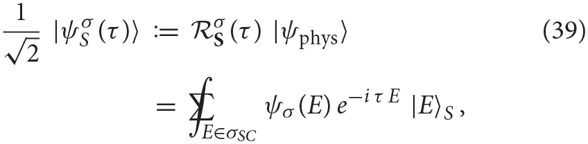
In order to complete the reduction to the states of the relational Heisenberg picture, and thus also complete step 2. above, we “project” out the redundant clock factor of the trivialized states by projecting onto the classical gauge-fixing condition T = τ (see Supplementary Material for a discussion of the classical gauge-fixing). That is, we now proceed as in the Page-Wootters reduction and condition states in the trivialized physical Hilbert space ${{T}}_{T,ϵ}({{H}}_{\text{phys}})$ on the clock reading τ, separating positive and negative frequency modes. Altogether, the quantum symmetry reduction map takes the form

$\begin{array}{ll}{{R}}_H^{\sigma }≔e^{-i\tau s{\in }^2/2}\left(\langle \tau ,\sigma |\otimes I_S\right){{T}}_{T,\in }.& (51)\end{array}$

Using that

$\begin{array}{ll}\langle \tau ,\sigma |p_t=-{\sigma }^{\prime }ϵ\rangle ={\delta }_{\sigma {\sigma }^{\prime }}\sqrt{ϵ}{e}^{i\tau s{ϵ}^2/2},& (52)\end{array}$

which is another reason why ϵ > 0 is chosen, in Equation (50) one finds τ-independent system states

as appropriate for a Heisenberg picture (compare with Equation 39). This is also the reason why, in contrast to the Page-Wootters reduction in Equation (38), we do not label the quantum deparametrization map with a τ, despite the latter a priori appearing on the right hand side of Equation (51) and why we equip it with an H label. The factor $1/\sqrt{2}$ has again been introduced for normalization purposes. Since the wave function

$\begin{array}{ll}{\psi }_S^{\sigma }(E)\equiv \sqrt{2}{\psi }_{\sigma }(E),& (54)\end{array}$

is square-integrable/summable, it is clear that $|{\psi }_S^{\sigma }\rangle$ is an element of the physical system Hilbert space ${{H}}_{S,\sigma }^{\text{phys}}$, corresponding to the σ-sector. We therefore also have ${{R}}_{\text{H}}^{\sigma }(\tau ):{{H}}_{\text{phys}}\to {{H}}_{S,\sigma }^{\text{phys}}$, just as in Page-Wootters reduction. Using Lemmas 6 and 7, it is now also clear how to invert the quantum symmetry reduction—at least per σ-sector:

${({{R}}_H^{\sigma })}^{-1}≔{{T}}_{T,ϵ}^{-1}\left(\frac{1}{\sqrt{ϵ}}{|p_t=-\sigma ϵ\rangle }_C\otimes I_S\right)$

defines a map ${{H}}_{S,\sigma }^{\text{phys}}\to {{H}}_{\sigma }$, so that¹⁸

$\begin{array}{ll}{\left({{R}}_H^{\sigma }\right)}^{-1}|{\psi }_S^{\sigma }\rangle =\sqrt{2\theta }\left(-\sigma {\widehat{p}}_t\right)|{\psi }_{\text{phys}}\rangle .& (55)\end{array}$

Hence, from the physical system Hilbert space of the positive/negative frequency modes one can only recover the positive/negative frequency sector of the physical Hilbert space. Note that the inverse map is independent of τ in contrast to the Page-Wottters case.

More precisely, the following holds.

Lemma 8. The quantum symmetry reduction map is weakly equal to the Page-Wootters reduction map and an (inverse) system time evolution

$\begin{array}{l}{{R}}_H^{\sigma }\approx \langle \tau ,\sigma |\otimes U_S^{†}\left(\tau \right),\hfill \\ =U_S^{†}\left(\tau \right){{R}}_S^{\sigma }\left(\tau \right).\hfill \end{array}$

Similarly, the inverse of the quantum symmetry reduction is equal to a system time evolution and the inverse of the Page-Wootters reduction:

$\begin{array}{l}{\left({{R}}_H^{\sigma }\right)}^{-1}=\delta \left({\widehat{C}}_H\right)\left(|\tau ,\sigma \rangle \otimes U_S\left(\tau \right)\right)\hfill \\ ={\left({{R}}_S^{\sigma }\left(\tau \right)\right)}^{-1}{U}_S\left(\tau \right).\hfill \end{array}$

Hence

$\begin{array}{l}{({{R}}_H^{\sigma })}^{-1}{{R}}_H^{\sigma }\approx \theta (-\sigma {\widehat{p}}_t)\otimes I_S\end{array}$

and

${{R}}_H^{\sigma }{\left({{R}}_H^{\sigma }\right)}^{-1}|{\psi }_S^{\sigma }\rangle =|{\psi }_S^{\sigma }\rangle .$

Proof: The proof of Lemma 3 in Höhn et al. [7] applies here σ-sector wise. □

Given the Heisenberg-type states in Equation (53), we may consider evolving Heisenberg observables on ${{H}}_{S,\sigma }^{\text{phys}}$

$\begin{array}{ll}{\widehat{f}}_S^{\text{phys}}(\tau )=U_S^{†}(\tau ){\widehat{f}}_S^{\text{phys}}{U}_S(\tau ).& (56)\end{array}$

Indeed, the following theorem shows that these Heisenberg observables are equivalent to the relational Dirac observables on the σ-sector of the physical Hilbert space ${{H}}_{\sigma }$, thereby demonstrating that the quantum symmetry reduction map yields a relational Heisenberg picture. To this end, we employ these reduction maps and their inverses to define another encoding operation ${{E}}_{\text{H}}^{\sigma }:{L}\left({{H}}_{S,\sigma }^{\text{phys}}\right)\to {L}({{H}}_{\sigma })$,

$\begin{array}{ll}{{E}}_H^{\sigma }\left({\widehat{f}}_S^{\text{phys}}(\tau )\right)≔{({{R}}_H^{\sigma })}^{-1}{\widehat{f}}_S^{\text{phys}}(\tau ){{R}}_H^{\sigma }.& (57)\end{array}$

Theorem 3. Let ${\widehat{f}}_S\in {L}({{H}}_S)$. The quantum relational Dirac observable ${\widehat{F}}_{f_S,T}(\tau )$ acting on ${{H}}_{\text{phys}}$, Equation (31), reduces under ${{R}}_{\text{H}}^{\sigma }$ to the corresponding projected evolving observable in the Heisenberg picture on ${{H}}_{S,\sigma }^{\text{phys}}$, Equation (56), i.e.,

$\begin{array}{l}{{R}}_H^{\sigma }{\widehat{F}}_{f_S,T}(\tau ){({{R}}_H^{\sigma })}^{-1}={\Pi }_{{\sigma }_{SC}}{\widehat{f}}_S(\tau ){\Pi }_{{\sigma }_{SC}}\\ \equiv {\widehat{f}}_S^{\text{phys}}(\tau ).\end{array}$

Conversely, let ${\widehat{f}}_S^{\text{phys}}\left(\tau \right)\in {L}\left({{H}}_{S,\sigma }^{\text{phys}}\right)$ be any evolving Heisenberg observable. The encoding operation in Equation (57) of system observables coincides on the physical Hilbert space ${{H}}_{\text{phys}}$ with the quantum relational Dirac observables in Equation (31) projected into the σ-sector:

$\begin{array}{ll}{{E}}_H^{\sigma }\left({\widehat{f}}_S^{\text{phys}}(\tau )\right)\approx {\widehat{F}}_{f_S^{\text{phys}},T}^{\sigma }(\tau ).& (58)\end{array}$

Proof: The proof of Theorem 5 in Höhn et al. [7] applies here per σ-sector. □

Once more, the theorem establishes an equivalence between the full sets of relational Dirac observables relative to clock E_T on ${{H}}_{\sigma }$ and evolving Heisenberg observables on the physical system Hilbert space of the σ-modes ${{H}}_{S,\sigma }^{\text{phys}}$. Hence, one can recover the action of the relational Dirac observables only σ-sector wise from the Heisenberg observables.

Lemma 8 and Theorem 2 directly imply that we again have preservation of expectation values per σ-sector, as the following theorem shows.

Theorem 4. Let ${\widehat{f}}_S\in {L}({{H}}_S)$ and ${\widehat{f}}_S^{\text{phys}}(\tau )=U_S^{†}(\tau ){\Pi }_{{\sigma }_{SC}}{\widehat{f}}_S$ Π_σSCU_S(τ) be its associated evolving Heisenberg operator on ${{H}}_S^{\text{phys}}$. Then

$\langle {\psi }_{\text{phys}}|{\widehat{F}}_{f_S,T}^{\sigma }(\tau ){|{\varphi }_{\text{phys}}\rangle }_{\text{phys}}=\frac{1}{2}\langle {\psi }_S^{\sigma }|{\widehat{f}}_S^{\text{phys}}(\tau )|{\varphi }_S^{\sigma }\rangle ,$

where $|{\psi }_S^{\sigma }\rangle =\sqrt{2}{{R}}_H^{\sigma }|{\psi }_{\text{phys}}\rangle$.

Proof: The proof of Theorem 6 in Höhn et al. [7] applies here per σ-sector. □

Therefore, the quantum symmetry reduction map ${{R}}_{\text{H}}$ is an isometry, as we state in the following corollary.

Corollary 3. Setting ${\widehat{f}}_S={\Pi }_{{\sigma }_{SC}}$ in Theorem 4 yields

$\langle {\psi }_{\text{phys}}|\theta \left(-\sigma {\widehat{p}}_t\right)\otimes I_S{|{\varphi }_{\text{phys}}\rangle }_{\text{phys}}=\frac{1}{2}\langle {\psi }_S^{\sigma }|{\varphi }_S^{\sigma }\rangle ,$

where $|{\psi }_S^{\sigma }\rangle =\sqrt{2}{{R}}_{\text{H}}^{\sigma }|{\psi }_{\text{phys}}\rangle$. Hence,

${\langle {\psi }_{\text{phys}}|{\varphi }_{\text{phys}}\rangle }_{\text{phys}}=\frac{1}{2}{\displaystyle \sum _{\sigma }\langle {\psi }_S^{\sigma }|{\varphi }_S^{\sigma }\rangle }.$

Accordingly, we can work with normalized states in each reduced σ-sector and in the physical Hilbert space simultaneously.

In conclusion:

(1) Applying the quantum symmetry reduction map ${{R}}_{\text{H}}^{\sigma }$ to the clock-neutral picture on the physical Hilbert space ${{H}}_{\text{phys}}$ yields a relational Heisenberg picture with respect to the clock C on the physical system Hilbert space of the σ-modes, ${{H}}_{S,\sigma }^{\text{phys}}$.

(2) σ-sector wise, the relational quantum dynamics encoded in the relational Dirac observables on the physical Hilbert space is equivalent to the dynamics in the relational Heisenberg picture on the physical system Hilbert space.

(3) Given the invertibility of the reduction map, Theorem 4 formally shows that if ${\widehat{f}}_S^{\text{phys}}(\tau )$ is self-adjoint on ${{H}}_{S,\sigma }^{\text{phys}}$, then so is ${\widehat{F}}_{f_S,T}^{\sigma }(\tau )$ on ${{H}}_{\sigma }$.

5.1.4. Equivalence of Dynamics (ii) and (iii)

The previous subsections establish a σ-sector wise equivalence between the relational dynamics, on the one hand, in the clock-neutral picture of Dirac quantization and, on the other, the relational Schrödinger and Heisenberg pictures, obtained through Page-Wootters reduction and quantum deparametrization, respectively. It is thus evident that also the relational Schrödinger and Heisenberg pictures are indeed equivalent up to the unitary U_S(τ) as they should. This is directly implied by Lemma 8 which shows that the Page-Wotters and quantum symmetry reduction maps are (weakly) related by U_S(τ).

5.2. Quantum Analogs of Gauge-Fixing and Gauge-Invariant Extensions

In contrast to the classical constraint surface, the “quantum constraint surface” ${{H}}_{\text{phys}}$ is automatically gauge-invariant since the exponentiation of the symmetry generator Ĉ_H acts trivially on all physical states and Dirac observables. Nevertheless, extending the interpretation established in Höhn et al. [7], we can understand the quantum symmetry reduction map ${{R}}_{\text{H}}$ [and given their unitary relation, also ${{R}}_{\text{S}}^{\sigma }(\tau )$] as the quantum analog of a classical phase space reduction through gauge-fixing. For completeness, the latter procedure is explained in Supplementary Material for the class of models of this article. In particular, we may think of the physical system Hilbert space ${{H}}_{S,\sigma }^{\text{phys}}$ for the σ-sector as the quantum analog of the gauge-fixed reduced phase space obtained by imposing for example the gauge T = 0 on the classical σ-frequency sector ${{C}}_{\sigma }$¹⁹. Also classically, one obtains two identically looking gauge-fixed reduced phase spaces, one for each frequency sector. Consequently, the relational Schrödinger and Heisenberg pictures can both be understood as the quantum analog of a gauge-fixed formulation of a manifestly gauge-invariant theory.

In this light, Theorems 1 and 3 imply that the encoding operations of system observables in Equations (45) and (57) can be understood as the quantum analog of gauge-invariantly extending a gauge-fixed quantity (see also [7]). Similarly, the alternative physical inner product in the second line of Equation (47) is the quantum analog of a gauge-fixed version of the manifestly gauge-invariant physical inner product obtained through group averaging in Equation (18). Indeed, ${\displaystyle {\sum }_{\sigma }\langle {\psi }_{\text{phys}}|(|\tau ,\sigma \rangle \langle \tau ,\sigma |\otimes I_S){|{\varphi }_{\text{phys}}\rangle }_{\text{kin}}}$ is the (kinematical) expectation value of the ‘projector' onto clock time τ in physical states. However, it is clear from the unitarity of the Schrödinger dynamics on ${{H}}_{S,\sigma }^{\text{phys}}$ and Equation (47) that this inner product does not depend on τ (the “gauge”), in line with the interpretation of it being the quantum analog of a gauge-fixed version of a manifestly gauge-invariant quantity.

5.3. Interlude: Alternative Route

As an aside, we mention that there exists an alternative route to establishing a trinity for clock Hamiltonians quadratic in momenta. This again exploits the reducible representation on the physical Hilbert space. The σ-sector of ${{H}}_{\text{phys}}$ is defined by the constraint ${Ĉ}_{\sigma }={Ĥ}_C^{\prime }+{Ĥ}_S^{\prime }$, where ${Ĥ}_C^{\prime }≔\frac{{\widehat{p}}_t}{\sqrt{2}}$ and ${Ĥ}_S^{\prime }≔\sigma \sqrt{-s{Ĥ}_S}$. Clearly, ${Ĥ}_C^{\prime }$ is now a non-degenerate clock Hamiltonian. In Höhn et al. [7] we established the trinity for non-degenerate clock Hamiltonians and the σ-sector defined by ${Ĉ}_{\sigma }={Ĥ}_C^{\prime }+{Ĥ}_S^{\prime }$ yields a special case of that. This immediately implies a trinity per σ-sector, however, now relative to a clock POVM which is covariant with respect to ${Ĥ}_C^{\prime }$. It is evident that the covariant clock POVM is in this case defined through the eigenstates of $\widehat{t}$ which (up to a factor of $\sqrt{2}$) is also the first moment of the POVM. Indeed, the equivalence between the clock-neutral Dirac quantization and the relational Heisenberg picture has previously been established for models with quadratic clock Hamiltonians precisely in this manner in Höhn and Vanrietvelde [30] and Höhn [31] (for a related discussion see also [29, 38]). However, as mentioned in section 4.1, one either has to regularize the relational observables or write them as functions of affine, rather than canonical pairs of evolving degrees of freedom. This is a consequence of the square root nature of ${Ĥ}_S^{\prime }$. None of these extra steps were needed in the trinity construction of this article, which is based on a clock POVM which is covariant with respect to $s\frac{{\widehat{p}}_t^2}{2}$, rather than ${\widehat{p}}_t/\sqrt{2}$.

6. Relativistic Localization: Addressing Kuchař's Criticism

In his seminal review on the problem of time, Kuchař raised three criticisms against the Page-Wootters formalism [1]: the Page-Wootters conditional probability in Equation (37) (a) yields the wrong localization probabilities for a relativistic particle, (b) violates the Hamiltonian constraint, and (c) produces incorrect transition probabilities. As mentioned in the introduction, criticisms (b) and (c) have been resolved in Höhn et al. [7]—see Theorem 2 which extends the resolution of (b) to the present class of models.

Here, we shall now also address Kuchař's first criticism (a) on relativistic localization, which is more subtle to resolve. The main reason, as is well-known from the theorems of Perez-Wilde [92] and Malament [93] (see also the discussion in [94, 95]), is that there is no relativistically covariant position-operator-based notion of localization which is compatible with relativistic causality and positivity of energy. This is a key motivation for quantum field theory [90, 94]—and here a challenge for specifying what the “right” localization probability for a relativistic particle should be. Instead, one may resort to an approximate and relativistically non-covariant notion of localization proposed by Newton and Wigner [90, 91]. We will address criticism (a) by demonstrating that our formulation of the Page-Wootters formalism, based on covariant clocks for relativistic models, yields a localization in such an approximate sense.

For the sake of an explicit argument, we shall, just like Kuchař [1], focus solely on the free relativistic particle, whose Hamiltonian constraint reads (cf. Table 1)

$\begin{array}{l}{\widehat{C}}_H=-{\widehat{p}}_t^2+{\widehat{p}}^2+m^2,\end{array}$

where $\widehat{p}$ denotes the spatial momentum vector. However, the argument could be extended to the entire class of models considered in this manuscript. It is straightforward to check that the physical inner product Equation (18) reads in this case [31, 104]²⁰

$\begin{array}{l}{\langle {\varphi }_{\text{phys}}|{\psi }_{\text{phys}}\rangle }_{\text{phys}}={\displaystyle {\int }_{{ℝ}^3}\frac{d^{3}p}{2{\epsilon }_p}}[{\varphi }_{\text{kin}}^{*}({\epsilon }_p,p){\psi }_{\text{kin}}({\epsilon }_p,p)\\ +{\varphi }_{\text{kin}}^{*}(-{\epsilon }_p,p){\psi }_{\text{kin}}(-{\epsilon }_p,p)],& (59)\end{array}$

where ${\epsilon }_p=\sqrt{p^2+m^2}$ is the relativistic energy of the particle and the first and second term in the integrand correspond to negative and positive frequency modes, respectively. Fourier transforming to solutions to the Klein-Gordon equation in Minkowski space

$\begin{array}{l}{\psi }_{\text{phys}}^{\sigma }(t,x)=\frac{1}{{(2\pi )}^{3/2}}{\displaystyle {\int }_{{ℝ}^3}}\frac{d^{3}p}{2{\epsilon }_p}{e}^{i(x·p-\sigma t{\epsilon }_p)}{\psi }_{\text{kin}}(-\sigma {\epsilon }_p,p),\end{array}$

one may further check that [31, 104]

$\begin{array}{ll}{\langle {\varphi }_{\text{phys}}|{\psi }_{\text{phys}}\rangle }_{\text{phys}}={\left({\varphi }_{\text{phys}}^{+},{\psi }_{\text{phys}}^{+}\right)}_{\text{KG}}-{\left({\varphi }_{\text{phys}}^{-},{\psi }_{\text{phys}}^{-}\right)}_{\text{KG}},& (60)\end{array}$

where

$\begin{array}{l}{\left({\varphi }_{\text{phys}}^{\sigma },{\psi }_{\text{phys}}^{\sigma }\right)}_{\text{KG}}=i{\displaystyle {\int }_{{ℝ}^3}{d}^3}x[{\left({\varphi }_{\text{phys}}^{\sigma }(t,x)\right)}^{*}{\partial }_t{\psi }_{\text{phys}}^{\sigma }(t,x)\\ -{\left({\partial }_t{\varphi }_{\text{phys}}^{\sigma }(t,x)\right)}^{*}{\psi }_{\text{phys}}^{\sigma }(t,x)],& (61)\end{array}$

is the Klein-Gordon inner product in which positive frequency modes are positive semi-definite, negative frequency modes are negative semi-definite and positive and negative frequency modes are mutually orthogonal. The physical inner product is thus equivalent to the Klein-Gordon inner product (with correctly inverted sign for the negative frequency modes), which provides the correct and conserved normalization for the free relativistic particle²¹. This raises hopes that the conditional probabilities of the Page-Wootters formalism may yield the correct localization probability for the relativistic particle. Note that so far we have not yet made a choice of time operator.

Suppose now that the Minkowski time operator $\widehat{t}$, quantized as a self-adjoint operator on ${{H}}_{\text{kin}}$, is used to define the projector onto clock time t as e_C(t) = |t〉〈t| and e_x = |x〉〈x| is the projector onto position x. This time operator is not covariant with respect to the quadratic clock Hamiltonian. The conditional probability Equation (37) then becomes

$\begin{array}{ll}\text{Prob }\left(x\text{ when }t\right)=\frac{|{\psi }_{\text{phys}}(t,x){|}^2}{{\int }_{{ℝ}^3}{d}^3{x}^{\prime }|{\psi }_{\text{phys}}(t,x^{\prime }){|}^2},& (62)\end{array}$

where ψ_phys(t, x) = (〈t| ⊗ 〈x|) |ψ_phys〉 is a general solution to the Klein-Gordon equation. As Kuchař pointed out [1], while this would be the correct localization probability for a non-relativistic particle, it is the wrong result for a relativistic particle. Indeed, apart from not separating positive and negative frequency modes, which is necessary for a probabilistic interpretation e.g., if ψ_phys contains both positive and negative frequency modes then the denominator in Equation 62 is not conserved), Equation (62) neither coincides with the charge density of the Klein-Gordon current in Equation (61), nor with the Newton-Wigner approximate localization probability [90, 91]. In particular, one can not interpret a solution ψ_phys(t, x) to the Klein-Gordon equation as a probability amplitude to find the relativistic particle at position x at time t. The reason, as explained in Haag [90], is that the conserved density is the one in Equation (61) and ψ_phys and ∂_tψ_phys inside it are not only dependent, but related by a non-local convolution

${\partial }_t{\psi }_{\text{phys}}(t,x)={\displaystyle {\int }_{{ℝ}^3}{d}^3}{x}^{\prime }\epsilon (x-x^{\prime }){\psi }_{\text{phys}}(t,x^{\prime }),$

where ε(x − x′) is the Fourier transform of −iε_p.

By contrast, let us now exhibit what form of conditional probabilities the covariant clock POVM E_T of section 4.2 gives rise to. We now insert $e_C(\tau )={\displaystyle {\sum }_{\sigma }|\tau ,\sigma \rangle }\langle \tau ,\sigma |$ and, as before, e_x into the conditional probability Equation (37). The crucial difference between the covariant clock POVM E_T and the clock operator $\widehat{t}$ (which is covariant with respect to Ĉ_σ, but not Ĉ_H) is that the denominator of Equation (37) is equal to the physical inner product in the former case (see Corollary 2) but not in the latter²². Supposing that we work with normalized physical system states $\langle {\psi }_S^{\sigma }(\tau )|{\psi }_S^{\sigma }(\tau )\rangle =1$, Theorem 2 implies

$\begin{array}{l}\text{prob}\left(x\text{ when }\tau \right)=12{\displaystyle \sum _{\sigma }|}{\psi }_S^{\sigma }(\tau ,x){|}^2\\ ={\langle {\psi }_{\text{phys}}|{\widehat{F}}_{e_x,T}(\tau )|{\psi }_{\text{phys}}\rangle }_{{}_{\text{phys}}},& (63)\end{array}$

where ${\psi }_S^{\sigma }(\tau ,x)≔\sqrt{2}(\langle \tau ,\sigma |\otimes \langle x|)|{\psi }_{\text{phys}}\rangle$ and τ is now not Minkowski time. For concreteness, let us now focus on positive frequency modes. Using Equations (15) and (25), one obtains

$\begin{array}{ll}{\psi }_S^{+}(\tau ,x)=\frac{1}{{(2\pi )}^{3/2}}{\displaystyle {\int }_{{ℝ}^3}\frac{d^{3}p}{\sqrt{2{\epsilon }_p}}}{e}^{i(x·p-\tau {\epsilon }_p^2)}{\psi }_{\text{kin}}(-{\epsilon }_p,p).& (64)\end{array}$

This is almost the Newton-Wigner position space wave function for positive frequency modes, which relative to Minkowski time reads [90]

$\begin{array}{l}{\psi }_{\text{NW}}^{+}(t,x)={\displaystyle {\int }_{{ℝ}^3}{d}^{3}x}K(x-x^{\prime }){\psi }_{\text{phys}}^{+}(t,x^{\prime })\\ =\frac{1}{{(2\pi )}^{3/2}}{\displaystyle {\int }_{{ℝ}^3}\frac{d^{3}p}{\sqrt{2{\epsilon }_p}}}{e}^{i(x·p-t{\epsilon }_p)}{\psi }_{\text{kin}}(-{\epsilon }_p,p),& (65)\end{array}$

where K(x) is the Fourier transform of $\sqrt{2{\epsilon }_p}$. The key property of $|{\psi }_{\text{NW}}^{+}(t,x){|}^2$ is that, while not relativistically covariant, it does admit the interpretation of an approximate localization probability, with accuracy of the order of the Compton wave length, for finding the particle at position x at Minkowski time t [90, 91]. In particular,

$\begin{array}{l}{\left({\varphi }_{\text{phys}}^{+},{\psi }_{\text{phys}}^{+}\right)}_{\text{KG}}={\displaystyle {\int }_{{ℝ}^3}}{d}^{3}x{({\varphi }_{\text{NW}}^{+}(t,x))}^{*}{\psi }_{\text{NW}}^{+}(t,x),\end{array}$

i.e., the Klein-Gordon inner product assumes the usual Schrödinger form for the Newton-Wigner wave function.

Noting that due to Equation (19) we can heuristically view τ as t/ε_p, and comparing with Equation (65) we can interpret Equation (64) as a Newton-Wigner wave function as well, but expressed relative to a different time coordinate τ. Indeed, in line with this interpretation, we find that in this case too the physical inner product, Equation (60), for the positive frequency modes assumes the form of the standard Schrödinger theory inner product

$\begin{array}{l}{({\varphi }_{\text{phys}}^{+},{\psi }_{\text{phys}}^{+})}_{\text{KG}}={\displaystyle {\int }_{{ℝ}^3}}{d}^{3}x{({\varphi }_S^{+}(\tau ,x))}^{*}{\psi }_S^{+}(\tau ,x).\end{array}$

The analogous statement is true for the negative frequency modes. In that sense, Equation (63), in contrast to Equation (62), does admit the interpretation as a valid, yet approximate localization probability for the relativistic particle per frequency sector, just like in the standard Newton-Wigner case²³.

Accordingly, computing the conditional probabilities of the Page-Wootters formalism relative to the covariant clock POVM, rather than the non-covariant Minkowski time operator $\widehat{t}$, leads to an acceptable localization probability for a relativistic particle, thereby addressing also Kuchař's first criticism (a). Given the equivalence of the Page-Wootters formalism with the clock-neutral and the relational Heisenberg pictures, established through the trinity in section 5, this result also equips the quantum relational Dirac observables ${\widehat{F}}_{x,T}(\tau )$ and the evolving Heisenberg observables x(τ) with the interpretation of providing an approximate, Newton-Wigner type localization in Minkowski space.

7. Changing Quantum Clocks

So far we have worked with a single choice of clock. Let us now showcase how to change from the evolution relative to one choice of clock to that relative to another. Our discussion will apply to both the relational Schrödinger picture of the Page-Wootters formalism and the relational Heisenberg picture obtained through quantum deparametrization.

For concreteness, suppose we are given a Hamiltonian constraint of the form

$\begin{array}{ll}{\widehat{C}}_H=s_1\frac{{\widehat{p}}_1^2}{2}+s_2\frac{{\widehat{p}}_2^2}{2}+{\widehat{H}}_S,& (66)\end{array}$

where s_i = ±1 and ${\widehat{p}}_i$ denotes the momentum of clock subsystem C_i, i = 1, 2 and we have suppressed tensor products with identity operators. In particular, suppose Ĥ_S does not depend on either of the clock degrees of freedom. We will work with the covariant clock POVM of section 4.2 for both clock choices. For example, the constraints of the relativistic particle, the flat (k = 0) FLRW model with a massless scalar field and the Bianchi I and II models from Table 1 are of the above form²⁴. Our subsequent discussion will thus directly apply to these models.

Since we will exploit the Page-Wootters and symmetry reduction maps as “quantum coordinate maps” from the clock-neutral picture to the given “clock perspective,” we will be able to change from the description of the dynamics relative to one clock to that relative to another in close analogy to coordinate changes on a manifold. Due to the shape of the constraint in Equation (66) we now have superselection of Dirac observables and the physical Hilbert space across both the σ₁-frequency sectors of clock C₁ and the σ₂-frequency sectors of clock C₂. The physical Hilbert space takes the form

$\begin{array}{ll}{{H}}_{\text{phys}}={\displaystyle \underset{{\sigma }_1,{\sigma }_2}{\oplus }}{{H}}_{{\sigma }_1,{\sigma }_2},& (67)\end{array}$

where ${{H}}_{{\sigma }_1,{\sigma }_2}≔{{H}}_{{\sigma }_1}\cap {{H}}_{{\sigma }_2}$ is the overlap of the σ₁-sector of clock C₁ and the σ₂-sector of clock C₂. As we have seen the reduction maps are only invertible per frequency sector. Hence, we will only be able to change from a given σ₁-sector to the part of the σ₂-frequency sector which is contained in it. In other words, the “quantum coordinate changes” are restricted to each overlap ${{H}}_{{\sigma }_1,{\sigma }_2}$.

The method of changing temporal reference frames exhibited below is a direct extension of several previous works: Höhn and Vanrietvelde [30] and Höhn [31] developed the method σ-sector-wise for states and observables in the relational Heisenberg picture for Hamiltonians of the type in Equation (66) for two example models, but used clock operators canonically conjugate to the clock momenta ${\widehat{p}}_i$ (and thus not a clock POVM covariant with respect to the full clock Hamiltonian). The method of transforming relational observables from one clock description to another was demonstrated in Höhn and Vanrietvelde [30] and Höhn [31] for a subset of relational Dirac observables, paying, however, detailed attention to regularization necessities arising from time-of-arrival observables [18, 23, 117–119]. Our previous article [7] developed the method comprehensively for both states and observables for clock Hamiltonians with non-degenerate and continuous spectrum in both the relational Schrödinger and Heisenberg pictures; specifically, the transformation of arbitrary relational observables corresponding to relations between S and the clocks was developed for the corresponding class of models. In Castro-Ruiz et al. [47] the clock change method was exhibited for state transformations in the relational Schrödinger picture for ideal clocks whose Hamiltonian coincides with the clock momentum itself. Our discussion can also be viewed as a full quantum extension of the semiclassical method in Bojowald et al. [32, 33] and Höhn et al. [34] which is equivalent at semiclassical order, however, also applies to clock functions which are non-monotonic, i.e., have turning points, in contrast to the other works mentioned (See [70–72, 74] for related spatial quantum frame changes).

In particular, owing to our focus on covariant clock POVMs, all the results and proofs [7] apply σ-sector-wise to the present case. However, we will also study novel effects, such as the temporal frame dependence of comparing clock readings.

7.1. State Transformations

Denote by ${{R}}_I^{{\sigma }_i}$, where I ∈ {S, H}, the Page-Wootters or quantum symmetry reduction map to the σ_i-sector of clock C_i. For notational simplicity, we drop the dependence of the Page-Wootters reduction on the clock reading τ_i of clock C_i for the moment. The temporal frame change (TFC) map ${\Lambda }_{I\to J}^{{\sigma }_i\to {\sigma }_j}:{{H}}_{C_j,{\sigma }_i}^{\text{phys}}\otimes {{H}}_{S,{\sigma }_i}^{\text{phys}}\to {{H}}_{C_i,{\sigma }_j}^{\text{phys}}\otimes {{H}}_{S,{\sigma }_j}^{\text{phys}}$ from clock C_i's σ_i-sector to clock C_j's σ_j-sector then reads

$\begin{array}{ll}{\Lambda }_{I\to J}^{{\sigma }_i\to {\sigma }_j}≔{{R}}_J^{{\sigma }_j}\circ {({{R}}_I^{{\sigma }_i})}^{-1}.& (68)\end{array}$

Here ${{H}}_{C_j,{\sigma }_i}^{\text{phys}}$ denotes the physical clock C_j Hilbert space corresponding to the σ_i-sector of clock C_i, i.e., the subspace of ${{H}}_{C_j}$ compatible with solutions to the constraint Equation (66) and similarly for the other Hilbert spaces. When I ≠ J in Equation (68), then the TFC map changes not only the temporal reference frame, but also between the corresponding relational Heisenberg and Schrödinger pictures. Let us write ${\Lambda }_I^{{\sigma }_i\to {\sigma }_j}≔{\Lambda }_{I\to I}^{{\sigma }_i\to {\sigma }_j}$ when no relational picture change takes place.

More explicitly, the TFC map from the σ₁-frequency sector of clock C₁ in the relational Schrödinger picture to the σ₂-frequency sector of clock C₂ in the relational Schrödinger picture takes the form

$\begin{array}{l}{\Lambda }_{\text{S}}^{{\sigma }_1\to {\sigma }_2}=(\langle {\tau }_2,{\sigma }_2|\otimes I_{C_{1}S})\delta ({\widehat{C}}_H)(|{\tau }_1,{\sigma }_1\rangle \otimes I_{C_{2}S}).\end{array}$

Here we have made use of Equations (38) and (42) and the covariant clock states Equation (25) for both clocks. The reduced states transform under this map as follows:

$\begin{array}{ll}\left(\theta (-{\sigma }_1{\widehat{p}}_1)\otimes I_S\right)|{\psi }_{C_{1}S|C_2}^{{\sigma }_2}({\tau }_2)\rangle ={\Lambda }_S^{{\sigma }_1\to {\sigma }_2}|{\psi }_{C_{2}S|C_1}^{{\sigma }_1}({\tau }_1)\rangle ,& (69)\end{array}$

where we made use of Equation (43) and $|{\psi }_{C_{j}S|C_i}^{{\sigma }_i}({\tau }_i)\rangle$ is the relational Schrödinger picture state of clock C_j and system S relative to clock C_i, which is chosen as the temporal reference frame, in its σ_i-sector. In other words, the Heaviside-function on the l.h.s. highlights that we can only map from the σ₁-sector of clock C₁ to that part of the σ₂-sector of clock C₂ which is contained in the σ₁-sector of clock C₁. This is clear, because any reduction map is only invertible on its associated σ-sector: from the σ₁ relational Schrödinger picture one can only recover the σ₁-sector of the physical Hilbert space. Hence, the subsequent Page-Wootters reduction map to the σ₂-sector of clock C₂ in Equation (68) can then only yield information in the overlap of the σ₁- and σ₂-sectors in the physical Hilbert space (see also [30, 31] for explicit examples of this situation in the relational Heisenberg picture). This is a manifestation of the superselection across both the σ₁- and the σ₂-sectors.

Similarly, the TFC map from the σ₁-frequency sector of clock C₁ in the relational Heisenberg picture to the σ₂-frequency sector of clock C₂ in the relational Heisenberg picture reads

$\begin{array}{l}{\Lambda }_H^{{\sigma }_1\to {\sigma }_2}=\left(\langle {\tau }_2,{\sigma }_2|\otimes U_{C_{1}S}^{\mathrm{†}}({\tau }_2)\right)\\ \times \delta ({\widehat{C}}_H)\left(|{\tau }_1,{\sigma }_1\rangle \otimes U_{C_{2}S}({\tau }_1)\right)& (70)\end{array}$

where we have made use of Lemma 8. Using the same lemma, the reduced states transform under this map in complete analogy to Equation (69)

$[\theta (-{\sigma }_1{\widehat{p}}_1)\otimes I_S]|{\psi }_{C_{1}S|C_2}^{{\sigma }_2}\rangle ={\Lambda }_S^{{\sigma }_1\to {\sigma }_2}|{\psi }_{C_{2}S|C_1}^{{\sigma }_1}\rangle ,$

with $U_{C_{j}S}({\tau }_i)≔exp\left[-i{\tau }_i(s_j\frac{{\widehat{p}}_j^2}{2}+{Ĥ}_S)\right]$ the evolution operator of the composite system of clock C_j and system S relative to clock C_i.

Note that, interpreting the reduction maps as the “quantum coordinate maps” taking one from the clock-neutral physical Hilbert space to a specific “clock perspective,” any such TFC map in Equation (68) takes the same compositional form as coordinate changes on a manifold. In particular, any such temporal frame change proceeds by mapping via the clock-neutral physical Hilbert space in analogy to how coordinate changes always proceed via the manifold (see Figure 3). This observation lies at the heart of the perspective-neutral approach to quantum reference frame changes [7, 30, 31, 71, 72]. It is also the reason why we may interpret the physical Hilbert space as a clock-neutral structure, providing a description of the dynamics prior to having chosen a temporal reference frame relative to which the other degrees of freedom evolve. In line with this, in terms of different one-parameter families of relational Dirac observables, the physical Hilbert space contains the complete information about the dynamics relative to all the different possible clock choices at once.

FIGURE 3

Figure 3. Schematic representation of a temporal frame change, as defined through Equation (68). The figure encompasses both the relational Schrödinger picture of the Page-Wotters formalism and the relational Heisenberg picture of the quantum deparametrization (as well as their mixtures). Viewing the reduction maps ${{R}}_I^{{+}_i}$ as quantum coordinate maps, any such temporal frame change takes the form of a quantum coordinate transformation from the description relative to clock C₁ to the one relative to clock C₂. Just as coordinate transformation pass through the reference-frame-neutral manifold, the quantum coordinate transformations pass through the clock-neutral physical Hilbert space in line with the general discussion of the clock-neutral structure and quantum general covariance in section 2. Due to the double superselection rule, the quantum coordinate transformations have to preserve the overlaps of the frequency sectors of C₁ and C₂. Here we illustrate the example of the overlap of the positive frequency sectors of both clocks, so that the corresponding frame transformation passes through ${{H}}_{{+}_1,{+}_2}$ (cf. Equation 67).

7.2. Observable Transformations

Just as we transformed reduced states from the perspective of one clock to the perspective of another by passing through the gauge-invariant physical Hilbert space (see Figure 3), we now transform the description of observables relative to one clock to that relative to the other by passing through the gauge-invariant algebra of Dirac observables on the physical Hilbert space. The observable transformations will thus be dual to the state transformations. The idea is always that we describe the same physics, encoded in the gauge-invariant states and observables of the clock-neutral physical Hilbert space, but relative to different temporal frames. Again, we have to pay attention to the two superselection rules on the clock-neutral physical Hilbert space and we will demonstrate the observable transformations separately for the relational Schrödinger and Heisenberg pictures.

7.2.1. Observable Transformations in the Relational Schrödinger Picture

Suppose we are given an observable ${Ô}_{C_{2}S|C_1}^{\text{phys}}$ describing certain properties of the composite system C₂S in the relational Schrödinger picture of clock C₁ in either frequency sector of the latter²⁵. Owing to Theorem 1, we can write this as a reduction of a corresponding relational Dirac observable on ${{H}}_{\text{phys}}$:

${{R}}_S^{{\sigma }_1}\left({\tau }_1\right){\widehat{F}}_{O_{C_{2}S|C_1},T_1}({\tau }_1){\left({{R}}_S^{{\sigma }_1}({\tau }_1)\right)}^{-1}={\widehat{O}}_{C_{2}S|C_1}^{\text{phys}}.$

We can now also map the same relational Dirac observable into the σ₂-sector of the relational Schrödinger picture of clock C₂:

$\begin{array}{ll}{\widehat{O}}_{C_{1}S|C_2}^{\text{phys}}({\tau }_1,{\tau }_2):={{R}}_S^{{\sigma }_2}\left({\tau }_2\right){\widehat{F}}_{O_{C_{2}S|C_1},T_1}({\tau }_1){\left({{R}}_S^{{\sigma }_2}({\tau }_2)\right)}^{-1}.& (71)\end{array}$

The result will be the image of the original observable ${Ô}_{C_{2}S|C_1}^{\text{phys}}$, describing properties of C₂S relative to C₁, in the “perspective” of clock C₂. Hence, if ${Ô}_{C_{2}S|C_1}^{\text{phys}}$ depends non-trivially on C₂, an indirect self-reference effect occurs in the last equation [7]. Notice that, while the original observable in the Schrödinger picture of C₁ is independent of the evolution parameter τ₁, the description of that same observable in the Schrödinger picture relative to clock C₁ will generally depend on both evolution parameters τ₁, τ₂. The dependence on τ₁ is a consequence of it being the reduction of a relational Dirac observable with evolution parameter τ₁, but into the “perspective” of C₂. The possible τ₂ dependence may arise as a consequence of said indirect self-reference. For example, suppose ${Ô}_{C_{2}S|C_1}^{\text{phys}}={\widehat{T}}_2\otimes I_S$ so that the relational Dirac observable is ${\widehat{F}}_{O_{C_{2}S|C_1},T_1}({\tau }_1)={\widehat{F}}_{T_2,T_1}({\tau }_1)$. The observable on the l.h.s. in Equation (71) then describes how the first moment operator ${\widehat{T}}_2$ associated with C₂ evolves relative to C₁ from the “perspective” of C₂; this certainly should yield a τ₁ dependence. We will explain this in more detail shortly.

Taking into account the two superselection rules across the σ₁- and σ₂-sectors, these observations imply that observable transformations from the relational Schrödinger picture of the σ₁-sector of clock C₁ into the relational Schrödinger picture of the σ₂-sector of clock C₂ read

$\begin{array}{l}{\Lambda }_{\text{S}}^{{\sigma }_1\to {\sigma }_2}{Ô}_{C_{2}S|C_1}^{\text{phys}}{\left({\Lambda }_{\text{S}}^{{\sigma }_1\to {\sigma }_2}\right)}^{-1}={\left({\Lambda }_{\text{S}}^{{\sigma }_2\to {\sigma }_1}\right)}^{-1}{Ô}_{C_{2}S|C_1}^{\text{phys}}{\Lambda }_{\text{S}}^{{\sigma }_2\to {\sigma }_1}\\ ={{R}}_{\text{S}}^{{\sigma }_2}({\tau }_2)\circ {\left({{R}}_{\text{S}}^{{\sigma }_1}({\tau }_1)\right)}^{-1}{Ô}_{C_{2}S|C_1}^{\text{phys}}{{R}}_{\text{S}}^{{\sigma }_1}({\tau }_1)\bullet {\left({{R}}_{\text{S}}^{{\sigma }_2}({\tau }_2)\right)}^{-1}\\ ={{R}}_{\text{S}}^{{\sigma }_2}({\tau }_2){{E}}_{\text{S}}^{{\tau }_1,{\sigma }_1}\left({Ô}_{C_{2}S|C_1}^{\text{phys}}\right){\left({{R}}_{\text{S}}^{{\sigma }_2}({\tau }_2)\right)}^{-1}\\ \approx {{R}}_{\text{S}}^{{\sigma }_2}({\tau }_2){\widehat{F}}_{O_{C_{2}S|C_1},T_1}({\tau }_1)\left(\theta (-{\sigma }_1{\widehat{p}}_1)\otimes I_{C_{2}S}\right){\left({{R}}_{\text{S}}^{{\sigma }_2}({\tau }_2)\right)}^{-1}\\ =\left(\theta (-{\sigma }_1{\widehat{p}}_1)\otimes I_S\right){Ô}_{C_{1}S|C_2}^{\text{phys}}({\tau }_1,{\tau }_2).& (72)\end{array}$

In the second line we made use of Equation (45), in the third of Theorem 1, and in the fourth of Equation (71) and the fact that $\theta (-{\sigma }_1{\widehat{p}}_1)$ commutes with the reduction map of the C₂ clock and with ${\widehat{F}}_{O_{C_{2}S|C_1},T_1}({\tau }_1)$ (see Lemma 5).

Observe that the structure of this transformation shows that reduced observables relative to one clock will transform always via the gauge-invariant Dirac observable algebra to reduced observables relative to another clock.

Using Equations (38), (42), and (45), we can write this transformation as

$\begin{array}{l}\left(\theta (-{\sigma }_1{\widehat{p}}_1)\otimes I_S\right){\widehat{O}}_{C_{1}S|C_2}^{\text{phys}}({\tau }_1,{\tau }_2)=\langle {\tau }_2,{\sigma }_2\delta ({\widehat{C}}_H)\\ \left(|{\tau }_1,{\sigma }_1\text{}\rangle \langle {\tau }_1,{\sigma }_1|\otimes {\widehat{O}}_{C_{2}S|C_1}^{\text{phys}}\right)\delta ({\widehat{C}}_H)|{\tau }_2,{\sigma }_2\rangle .& (73)\end{array}$

This transformation reveals that expectation values are preserved in the following manner:

$\begin{array}{l}\langle {\psi }_{C_{1}S|C_2}^{{\sigma }_2}({\tau }_2)|\left(\theta (-{\sigma }_1{\widehat{p}}_1)\otimes I_S\right){Ô}_{C_{1}S|C_2}^{\text{phys}}({\tau }_1,{\tau }_2)|{\varphi }_{C_{1}S|C_2}^{{\sigma }_2}({\tau }_2)\rangle \\ =\langle {\psi }_{C_{2}S|C_1}^{{\sigma }_1}({\tau }_1)|\left(\theta (-{\sigma }_2{\widehat{p}}_2)\otimes I_S\right){Ô}_{C_{2}S|C_1}^{\text{phys}}(\theta (-{\sigma }_2{\widehat{p}}_2)\otimes I_S)|{\varphi }_{C_{2}S|C_1}^{{\sigma }_1}({\tau }_1)\rangle .& (74)\end{array}$

The projectors onto the σ₂-sector on the r.h.s. appears because the C₂ reduction map in Equation (72) induces such a projection (compare this with the state transformations Equation (69) which are dual). In other words, only the physical information in the overlap of the σ₁- and σ₂-sector is preserved when changing from the description relative to clock C₁ to one relative to clock C₂, or vice versa. Once more, this is a direct consequence of the double superselection rule induced by the shape of the constraint Equation (66).

7.2.2. Observable Transformations in the Relational Heisenberg Picture

The argumentation for the relational Heisenberg picture proceeds in complete analogy. We thus just quote the results, which immediately follow from those of the previous subsection through use of Lemma 8. Of course, in this case, the reduced observables have an explicit dependence on the evolution parameter (Equation 56).

The observable transformations from the relational Heisenberg picture of the σ₁-sector of clock C₁ into the relational Heisenberg picture of the σ₂-sector of clock C₂ are given by

$\begin{array}{l}{\Lambda }_{\text{H}}^{{\sigma }_1\to {\sigma }_2}{Ô}_{C_{2}S|C_1}^{\text{phys}}({\tau }_1){\left({\Lambda }_{\text{H}}^{{\sigma }_1\to {\sigma }_2}\right)}^{-1}\\ \approx {{R}}_{\text{H}}^{{\sigma }_2}{\widehat{F}}_{O_{C_{2}S|C_1},T_1}({\tau }_1)\left(\theta (-{\sigma }_1{\widehat{p}}_1)\otimes I_{C_{2}S}\right){\left({{R}}_{\text{H}}^{{\sigma }_2}\right)}^{-1}\\ =\left(\theta (-{\sigma }_1{\widehat{p}}_1)\otimes I_S\right)U_{C_{1}S}^{†}({\tau }_2){Ô}_{C_{1}S|C_2}^{\text{phys}}({\tau }_1,{\tau }_2)U_{C_{1}S}({\tau }_2)\\ =:\left(\theta (-{\sigma }_1{\widehat{p}}_1)\otimes I_S\right){Ô}_{C_{1}S|C_2}^{\text{H}}({\tau }_1,{\tau }_2),& (75)\end{array}$

where ${Ô}_{C_{1}S|C_2}^{\text{phys}}({\tau }_1,{\tau }_2)$ is given by Equations (71) and (73). Thanks to the double superselection rule, this transformation preserves expectation values again per overlap of a σ₁- with a σ₂-sector, in obvious analogy to Equation (74).

7.3. Occurrence of Indirect Clock Self-Reference

Finally, let us now come back to the indirect self-reference effect of clock C₂ alluded to above. The following theorem, which is adapted from Höhn et al. [7] and whose proof applies here per pair of σ₁- and σ₂-sector, reveals the necessary and sufficient conditions for this indirect self-reference to occur:

Theorem 5. Consider an operator ${Ô}_{C_{2}S|C_1}^{\text{phys}}\in {L}({{H}}_{C_2}^{\text{phys}}\otimes {{H}}_S^{\text{phys}})$ of the composite system C₂S described from the perspective of clock C₁. From the perspective of clock C₂, this operator is independent of τ₂, so that ${Ô}_{C_{1}S|C_2}^{\text{phys}}({\tau }_1,{\tau }_2)={Ô}_{C_{1}S|C_2}^{\text{phys}}({\tau }_1)\in {L}({{H}}_{C_1}^{\text{phys}}\otimes {{H}}_S^{\text{phys}})$ if and only if

$\begin{array}{l}{Ô}_{C_{2}S|C_1}^{\text{phys}}={\displaystyle \sum _i}{\left({Ô}_{C_2|C_1}^{\text{phys}}\right)}_i\otimes {\left({\widehat{f}}_{S|C_1}^{\text{phys}}\right)}_i,\end{array}$

where ${({\widehat{f}}_{S|C_1}^{\text{phys}})}_i$ is an operator on ${{H}}_S^{\text{phys}}$ and ${({Ô}_{C_2|C_1}^{\text{phys}})}_i$ is a constant of motion, $\left[{({Ô}_{C_2|C_1}^{\text{phys}})}_i,s_2\frac{{\widehat{p}}_2^2}{2}\right]=0$. Furthermore, in this case the transformed observable reads

$\begin{array}{l}[\theta (-{\sigma }_1{\widehat{p}}_1)\otimes I_S]{Ô}_{C_{1}S|C_2}^{phys}({\tau }_1)\hfill \\ ={\Pi }_{{\sigma }_{C_{1}S{C}_2}}[\text{}{\displaystyle \sum }_i{G}_{C_{1}S}\text{}(|{\tau }_1,{\sigma }_1\rangle \langle {\tau }_1,\sigma {|}_1\otimes {({\widehat{f}}_{S|C_1}^{phys})}_i)\hfill \\ \langle t_2,{\sigma }_2|{({\widehat{O}}_{C_2|C_1}^{phys})}_i\delta ({\widehat{C}}_H)|t_2,{\sigma }_2\rangle ]{\Pi }_{{\sigma }_{C_{1}S{C}_2}},\hfill & (76)\end{array}$

where ${\Pi }_{{\sigma }_{C_{1}S{C}_2}}=\theta [-s_2\left(s_1\frac{{\widehat{p}}_1^2}{2}+{Ĥ}_S\right)]$ is the projector onto the physical subspace of ${{H}}_{C_1}\otimes {{H}}_S$, |t₂, σ₂〉 is an arbitrary σ₂-sector clock state of C₂, and ${{G}}_{C_{1}S}$ is the G-twirl over the group generated by the evolution generator $s_1\frac{{\widehat{p}}_1^2}{2}+{Ĥ}_S$ of the composite system C₁S.

That is to say, the indirect self-reference effect and thus τ₂-dependence of Equation (72) is absent if and only if the relational Dirac observable encoding how C₂S properties evolve relative to C₁ does not contain any degrees of freedom of clock C₂ that evolve.

When ${Ô}_{C_{2}S|C_1}^{\text{phys}}=I_{C_2}\otimes {\widehat{f}}_{S|C_1}^{\text{phys}}$, i.e., only the evolution of system degrees of freedom relative to C₁ is described, Theorem 5 entails that the transformation to the description relative to C₂ simplifies as follows:

$\begin{array}{l}\left(\theta (-{\sigma }_1{\widehat{p}}_1)\otimes I_S\right){Ô}_{C_{1}S|C_2}^{\text{phys}}({\tau }_1)=\\ {\Pi }_{{\sigma }_{C_{1}S{C}_2}}{{G}}_{C_{1}S}(|{\tau }_1,{\sigma }_1\rangle \langle {\tau }_1,{\sigma }_1|\otimes {\widehat{f}}_{S|C_1}^{\text{phys}}){\Pi }_{{\sigma }_{C_{1}S{C}_2}}.\end{array}$

In particular, the transformed system observable is perspective independent, i.e., its description relative to C₁ and C₂ coincide if and only if it is a constant of motion (see [7] for the proof of this statement, which again applies here per pair of σ₁- and σ₂-sector):

Corollary 4. An operator of C₂S relative to C₁

$\begin{array}{l}{Ô}_{C_{2}S|C_1}^{\text{phys}}=I_{C_2}\otimes {\widehat{f}}_{S|C_1}^{\text{phys}}.\end{array}$

transforms under a temporal frame change map to the perspective of C₂ as follows

$\begin{array}{l}{Ô}_{C_{1}S|C_2}^{\text{phys}}=I_{C_1}\otimes {\widehat{f}}_{S|C_2}^{\text{phys}},\end{array}$

where ${\widehat{f}}_{S|C_1}^{\text{phys}}={\widehat{f}}_{S|C_2}^{\text{phys}}$ if and only if ${\widehat{f}}_{S|C_1}^{\text{phys}}$ is a constant of motion, $[{\widehat{f}}_{S|C_1}^{\text{phys}},{Ĥ}_S]=0$.

Theorem 5 translates as follows into the relational Heisenberg picture (see [7] for the proof which applies here per pair of σ₁- and σ₂-sector):

Corollary 5. Let ${Ô}_{C_{2}S|C_1}^{\text{phys}}({\tau }_1)\in {L}({{H}}_{C_2}^{\text{phys}}\otimes {{H}}_S^{\text{phys}})$ be an operator describing the dynamics of properties of the composite system C₂S relative to C₁ in the Heisenberg picture. Under a temporal frame change Equation (75) to the perspective of C₂, this operator transforms to an operator ${Ô}_{C_{1}S|C_2}^H({\tau }_1,{\tau }_2)$ that satisfies the Heisenberg equation of motion in clock C₂ time τ₂ without an explicitly τ₂ dependent term,

$\begin{array}{l}\frac{d}{d{\tau }_2}{Ô}_{C_{1}S|C_2}^{\text{H}}({\tau }_1,{\tau }_2)=i\left[s_2\frac{{\widehat{p}}_2^2}{2}+{\widehat{H}}_S,{Ô}_{C_{1}S|C_2}^{\text{H}}({\tau }_1,{\tau }_2)\right],\end{array}$

if and only if

$\begin{array}{l}{Ô}_{C_{2}S|C_1}^{\text{phys}}({\tau }_1)={\displaystyle \sum _i}{\left({Ô}_{C_2|C_1}^{\text{phys}}\right)}_i\otimes {\left({\widehat{f}}_{S|C_1}^{\text{phys}}({\tau }_1)\right)}_i,\end{array}$

and ${\left({Ô}_{C_2|C_1}^{\text{phys}}\right)}_i$ is a constant of motion, $[s_1\frac{{\widehat{p}}_1^2}{2},{Ô}_{C_2|C_1}^{\text{phys}}]=0$.

The interpretation of the transformations is of course completely analogous to the relational Schrödinger picture.

7.4. Application: Comparing Clock Readings

One application of the temporal frame change method developed above is comparing readings of different clocks. This is also a prerequisite for developing a notion of clock synchronization.

For example, we may wish to compare the evolution of some system property ${\widehat{f}}_S$ relative to clock C₁ with ${\widehat{f}}_S$ relative to clock C₂. These two relational evolutions will be encoded in two one-parameter families of Dirac observable of the form ${\widehat{F}}_{I_{C_2}\otimes f_S,T_1}({\tau }_1)$ and ${\widehat{F}}_{I_{C_1}\otimes f_S,T_2}({\tau }_2)$. In order to relate these two dynamics, we need a consistent method for relating the different clock readings τ₁, τ₂. While classically, there is an unambiguous way to answer the question “what is the value of the reading τ₂ of clock C₂, when clock C₁ reads τ₁?” namely by setting τ₂(τ₁) ≔ F_T2,T1(τ₁), this is not so in the quantum theory because both clocks are now described in terms of quantum operators and their relation depends on the quantum state. In fact, we shall argue shortly that comparing clock readings is generally dependent on the choice of temporal frame (here either C₁ or C₂) in the quantum theory.

7.4.1. Three Ways of Comparing Clock Readings

To address this conundrum in the quantum theory, let us recall the conditional probabilities in Equation (37) and ask for the probability that C₂ reads τ₂ when C₁ reads τ₁ (ignoring frequency sectors for simplicity for the moment):

$\begin{array}{l}P(T_2={\tau }_2|T_1={\tau }_1)\\ =\langle {\psi }_{\text{phys}}|e_{C_1}({\tau }_1)\otimes e_{C_2}({\tau }_2)\otimes I_S{|{\psi }_{\text{phys}}\rangle }_{\text{kin}}\\ =P(T_1={\tau }_1|T_2={\tau }_2).& (77)\end{array}$

Here we have assumed that the physical state is normalized such that by Corollary 2 also the reduced states in the Schrödinger picture of either clock are normalized.

Comparing clock readings. Given the conditional probabilities Equation (77), we may consider the following three generally distinct options for comparing clock readings.

(A) The clock reading of C₂ when C₁ reads τ₁ is defined to be the value of τ₂ that maximizes the conditional probability P(T₂ = τ₂|T₁ = τ₁). This assumes the distribution to have a unique maximal peak.

(B) The clock reading of C₂ when C₁ reads τ₁ is defined to be the expectation value

$\begin{array}{ll}{\tau }_2({\tau }_1)≔{\displaystyle {\int }_{ℝ}}d{\tau }^{\prime }{\tau }^{\prime }P(T_2={\tau }^{\prime }|T_1={\tau }_1).& (78)\end{array}$

(C) The clock reading of C₂ when C₁ reads τ₁ is defined to be ${\left({\tau }_2^{(n)}({\tau }_1)\right)}^{1/n}$ for n > 1, where

$\begin{array}{ll}{\tau }_2^{(n)}({\tau }_1)≔{\displaystyle {\int }_{ℝ}}d{\tau }^{\prime }{({\tau }^{\prime })}^{n}P(T_2={\tau }^{\prime }|T_1={\tau }_1)& (79)\end{array}$

is the nth-moment of the conditional probability distribution in Equation (77).

Relating different clock readings in terms of expectation values, as in (B), is arguably the most natural choice and has originally been discussed in Höhn and Vanrietvelde [30], Höhn [31], Bojowald et al. [32, 33], Höhn et al. [34], and Smith and Ahmadi [45]; we expand on this here.

Clearly, the two definitions (A) and (B) only agree when the conditional probability distribution is peaked on the expectation value. Furthermore, all three definitions (A)–(C) agree in the special case that $P(T_2={\tau }^{\prime }|T_1={\tau }_1)=\delta ({\tau }^{\prime }-{\tau }_1)$, i.e., when there are no fluctuations in the conditional probability distribution.

7.4.2. Comparing Clock Readings for Quadratic Clock Hamiltonians

Let us now explore these definitions in our present class of models defined by Equation (66), taking into account the different frequency sectors again. Minding the double superselection rule, we replace Equation (77) by

$\begin{array}{l}{P}_{{\sigma }_1,{\sigma }_2}(T_2={\tau }_2|T_1={\tau }_1)\\ =\langle {\psi }_{\text{phys}}|e_{C_1}^{{\sigma }_1}({\tau }_1)\otimes e_{C_2}^{{\sigma }_2}({\tau }_2)\otimes I_S{|{\psi }_{\text{phys}}\rangle }_{\text{kin}}\\ =\langle {\psi }_{{\sigma }_1,{\sigma }_2}|e_{C_1}({\tau }_1)\otimes e_{C_2}({\tau }_2)\otimes I_S{|{\psi }_{{\sigma }_1,{\sigma }_2}\rangle }_{\text{kin}},& (80)\end{array}$

where $|{\psi }_{{\sigma }_1,{\sigma }_2}\rangle \in {{H}}_{{\sigma }_1,{\sigma }_2}$ lies in the overlap of the σ₁- and σ₂-sectors (see Equation 67) and $e_{C_i}^{{\sigma }_i}({\tau }_i)≔\frac{1}{2\pi }|{\tau }_i,{\sigma }_i\rangle \langle {\tau }_i,{\sigma }_i|$, i = 1, 2. We can then write the n^th-moment of the conditional probability distribution in Equations (78) and (79) for n ∈ ℕ, thus considering both definitions (B) and (C), as follows:

$\begin{array}{l}{\tau }_2^{(n)}({\tau }_1)={\displaystyle {\int }_{ℝ}}d{\tau }^{\prime }{({\tau }^{\prime })}^n{P}_{{\sigma }_1,{\sigma }_2}(T_2={\tau }^{\prime }|T_1={\tau }_1)\\ =\langle {\psi }_{C_{2}S|C_1}^{{\sigma }_1}({\tau }_1)|{\widehat{T}}_{2,{\sigma }_2}^{(n)}\otimes I_S|{\psi }_{C_{2}S|C_1}^{{\sigma }_1}({\tau }_1)\rangle \\ =\langle {\psi }_{{\sigma }_1,{\sigma }_2}|{\widehat{F}}_{T_2^{(n)}\otimes I_S,T_1}({\tau }_1)){|{\psi }_{{\sigma }_1,{\sigma }_2}\rangle }_{\text{phys}},& (81)\end{array}$

where by Equation (30)

$\begin{array}{l}{\widehat{T}}_{2,{\sigma }_2}^{(n)}=\frac{1}{2\pi }{\displaystyle {\int }_{ℝ}}dt{t}^n|t,{\sigma }_2\rangle \langle t,{\sigma }_2|\\ =\theta (-{\sigma }_2{\widehat{p}}_2){\widehat{T}}_2^{(n)}\theta (-{\sigma }_2{\widehat{p}}_2)\end{array}$

is the σ₂-sector nth-moment of the covariant clock POVM corresponding to C₂. In the second line of Equation (81) we have made use of Equations (38) and (80), while in the third line we invoked Theorem 2. Note that by Equation (74), the expression in Equation (81) defines an expectation value which is preserved during a temporal frame change between C₁ and C₂.

Thanks to Lemmas 3 and 4 we can write the nth-moment in Equation (81) also in the form

$\begin{array}{l}{\tau }_2^{(n)}({\tau }_1)=\langle {\psi }_{C_{2}S|C_1}^{{\sigma }_1}({\tau }_1)|{\widehat{T}}_{2,{\sigma }_2}^n\otimes I_S|{\psi }_{C_{2}S|C_1}^{{\sigma }_1}({\tau }_1)\rangle \\ =\langle {\psi }_{{\sigma }_1,{\sigma }_2}|{\widehat{F}}_{T_2^n\otimes I_S,T_1}({\tau }_1))|{{\psi }_{{\sigma }_1,{\sigma }_2}\rangle }_{\text{phys}},\end{array}$

as long as $|{\psi }_{C_{2}S|C_1}^{{\sigma }_1}({\tau }_1)\rangle \in \left({D}({\widehat{T}}_2^n)\cap {{H}}_{C_2}^{\text{phys}}\right)\otimes {{H}}_S^{\text{phys}}$. Since ${\left({\tau }_2^{(n)}({\tau }_1)\right)}^{1/n}\ne {\tau }_2({\tau }_1)$ for n > 1 for general states, definitions (B) and (C) will generically not be equivalent. In the sequel, we shall mostly consider definition (B) in extension of Höhn and Vanrietvelde [30], Höhn [31], Bojowald et al. [32, 33], Höhn et al. [34], and Smith and Ahmadi [45]. This seems to be the physically most appealing one, especially if an ensemble interpretation could be developed for the models under consideration. Definition (A) is only unambiguous when the conditional probability distribution has a single maximal peak and definition (C) is operationally unnatural and convoluted. That is, we set for the value of the reading of clock C₂ when C₁ reads τ₁:

$\begin{array}{ll}{\tau }_2({\tau }_1)≔{\tau }_2^{(1)}({\tau }_1).& (82)\end{array}$

The following discussion, however, qualitatively also applies to definition (C).

7.4.3. Comparing Clock Readings Is Temporal Frame Dependent

Notice that definitions (A)–(C) treat C₂ as the fluctuating subsystem. We can thus interpret them as providing a definition of the clock reading of C₂ relative to the temporal reference frame C₁. Conversely, we can of course switch the roles of C₁ and C₂ above and ask for the clock reading of C₁ relative to C₂. Resorting to definition (B), this would yield

$\begin{array}{ll}{\tau }_1({\tau }_2)={\displaystyle {\int }_{ℝ}}d{\tau }^{\prime }{\tau }^{\prime }{P}_{{\sigma }_1,{\sigma }_2}(T_2={\tau }_2|T_1={\tau }^{\prime }).& (83)\end{array}$

Dropping the labels of the arguments in Equations (81) and (83), both of which run over all of ℝ, it is important to note that τ₁(τ) and τ₂(τ) will generally not be the same functions of τ. This is because generally $P_{{\sigma }_1,{\sigma }_2}(T_2={\tau }^{\prime }|T_1=\tau )\ne P_{{\sigma }_1,{\sigma }_2}(T_2=\tau |T_1={\tau }^{\prime })$ in Equation (80). Said another way, the evolution of C₂ from the perspective of C₁ according to definition (B) may differ from the evolution of C₁ relative to C₂ (for the same physical state).

One might wonder whether the function τ₁(τ₂) in Equation (83) is the inversion of τ₂(τ₁) in Equation (81), i.e., obtained by solving τ₂(τ₁) for τ₁. Classically, this is certainly the case and it would entail that for a fixed clock reading ${\tau }_1^{*}$ of C₁ one finds ${\tau }_1({\tau }_2({\tau }_1^{*}))={\tau }_1^{*}$. Physically this would mean that both temporal reference frames C₁ and C₂ agree that when C₁ reads ${\tau }_1^{*}$, C₂ reads the value ${\tau }_2({\tau }_1^{*})$. This does occur in a special case when definitions (A)–(C) all coincide, namely when $P_{{\sigma }_1,{\sigma }_2}(T_2={\tau }_2({\tau }_1^{*})|T_1={\tau }^{\prime })=\delta ({\tau }^{\prime }-{\tau }_1^{*})$ in Equation (83) in which case expectation value, most probable value and the value defined through the nth-moment all agree. While this does happen in simple models with a high degree of symmetry between C₁ and C₂ [31], this will in more interesting cases not be the case because the physical state will generically have a different spread along the τ₁ and τ₂ axes [30, 32–34]. In our case this means that the wave function

${\psi }_{C_{2}S|C_1}^{{\sigma }_1,{\sigma }_2}({\tau }_1,{\tau }_2)≔\left(\langle {\tau }_1,{\sigma }_1|\otimes \langle {\tau }_2,{\sigma }_2|\otimes \langle {\varphi }_S|\right)|{\psi }_{\text{phys}}\rangle ,$

for some physical system state $|{\varphi }_S\rangle \in {{H}}_S^{\text{phys}}$, which can be viewed as either a wave function in the C₁ or C₂ relational Schrödinger picture, may have a different spread in τ₁ than in τ₂. In such a case we will generally find ${\tau }_1({\tau }_2({\tau }_1^{*}))\ne {\tau }_1^{*}$. This effect will occur in the class of models considered here because physical states need not have the same momentum distribution in p₁ and p₂ (and thus neither in τ₁ or τ₂) due to the presence of the system S. This effect has also been demonstrated in a semiclassical approach in various models in Bojowald et al. [32, 33] and Höhn et al. [34] where one finds discrepancies of the order of ℏ between ${\tau }_1^{*}$ and ${\tau }_1({\tau }_2^{*}={\tau }_2({\tau }_1^{*}))$.

In conclusion, this effect can be interpreted as a temporal frame dependence of comparing clock readings according to definition (B) [or (C)]: if from the perspective of the temporal reference frame defined by C₁ the clock C₂ reads ${\tau }_2({\tau }_1^{*})$ (computed according to Equation 81) when C₁ reads ${\tau }_1^{*}$, then conversely from the perspective of the temporal reference frame defined by C₂ the clock C₁ will not in general read ${\tau }_1^{*}$ when C₂ reads the value ${\tau }_2({\tau }_1^{*})$. That is, C₁ and C₂ will generally disagree about the pairings of their clock readings.

Let us now also briefly comment on the notion of quantum clock synchronization. Using the state dependent relation Equation (82), we could ask for which state would yield ${\tau }_2({\tau }_1^{*})={\tau }_1^{*}$ so that C₁ and C₂ read the same value when C₁ reads the value ${\tau }_1^{*}$. Even stronger, we could ask whether there are states for which τ₂(τ₁) = τ₁ + const, for all τ₁ ∈ ℝ, so that, up to a constant offset, C₁ and C₂ are always synchronized. Equation (81) tells us that this is the case if $P_{{\sigma }_1,{\sigma }_2}(T_2={\tau }^{\prime }|T_1={\tau }_1)=\delta ({\tau }^{\prime }-{\tau }_1-const)$. Again, while this happens in simple models [31], this will generically not happen for the models in the class which we are studying on account of the above observations concerning the frame dependence of comparing clock readings. Such a notion of synchronization is therefore too strong and can generally not be implemented. It will furthermore generally be frame dependent too.

7.4.4. Comparing a System's Evolution Relative to Two Clocks

Returning to our original ambition, it is thus more useful to employ the more general (frame dependent) clock comparison, according to definition (B), in order to compare the evolutions of S with respect to C₁ and C₂. Working in the relational Schrödinger picture, if $|{\psi }_{C_{2}S|C_1}^{{\sigma }_1}({\tau }_1^{*})\rangle$ is the initial state of C₂S from the perspective of C₁, then according to Equation (69) the corresponding initial state of C₁S from the perspective of C₂ is

$\begin{array}{l}\left(\theta (-{\sigma }_1{\widehat{p}}_1)\otimes I_S\right)|{\psi }_{C_{1}S|C_2}^{{\sigma }_2}({\tau }_2({\tau }_1^{*}))\rangle \\ ={{R}}_S^{{\sigma }_2}({\tau }_2({\tau }_1^{*}))\circ {\left({{R}}_S^{{\sigma }_1}({\tau }_1^{*})\right)}^{-1}|{\psi }_{C_{2}S|C_1}^{{\sigma }_1}({\tau }_1^{*})\rangle .& (84)\end{array}$

We can then evaluate the ‘same' reduced system observable $I_{C_i}\otimes {\widehat{f}}_S^{\text{phys}}$ in the two states, where i = 1 when evaluated relative to C₂ and vice versa (cf. Corollary 4), in order to compare the evolution of property ${\widehat{f}}_S^{\text{phys}}$ relative to the two clocks in different quantum states (which amount also to quantum states of the clocks). To avoid confusion, we emphasize, that $I_{C_i}\otimes {\widehat{f}}_S^{\text{phys}}$, i = 1, 2, correspond to two different relational Dirac observables ${\widehat{F}}_{I_{C_2}\otimes f_S,T_1}({\tau }_1)$ and ${\widehat{F}}_{I_{C_1}\otimes f_S,T_2}({\tau }_2)$ on the clock-neutral physical Hilbert space ${{H}}_{\text{phys}}$; in particular, the two are not related by the TFC map ${\Lambda }_{\text{S}}^{{\sigma }_1\to {\sigma }_2}$. Hence, by evaluating these two reduced observables in the relational Schrödinger states related via the TFC map ${\Lambda }_{\text{S}}^{{\sigma }_1\to {\sigma }_2}$ by Equation (84), we can compare two genuinely distinct relational dynamics. The construction in the relational Heisenberg picture is of course completely analogous.

In Höhn et al. [7] and Castro-Ruiz [47] a frame dependent temporal non-locality effect was exhibited for idealized clocks whose Hamiltonian is the unbounded momentum operator. For example, when clock C₂ is seen to be in a superposition of two peaked states and in a product relation with S from the perspective of C₁, then C₁S will generally be entangled as seen from the perspective of C₂ and undergo a superposition of time evolutions. This effect applies here per overlap of the different σ₁- and σ₂-sectors. It will be interesting to study how such a frame dependent temporal locality affects the (potentially frame dependent) comparison and synchronization of the clocks and the comparison of the evolutions of S relative to C₁ and C₂ in different quantum states, corresponding to different choices of the clock-neutral physical states. Such an exploration will appear elsewhere.

Finally, these temporal frame changes and clock synchronizations will be relevant in quantum cosmology. For example, recently it was pointed out that singularity resolution in quantum cosmology depends on the choice of clock which one uses to define a relational dynamics [77]. The different relational dynamics employed in Gielen and Menéndez-Pidal [77] can be interpreted as different choices of reduced dynamics in the sense of our relational Schrödinger/Heisenberg picture. Temporal frame changes as developed here can in principle be used to study the temporal frame dependence of the fate of cosmological singularities more systematically.

8. Conclusions

In this work we demonstrated the equivalence of three distinct approaches to relational quantum dynamics—relational Dirac observables, the Page-Wootters formalism, and quantum deparametrizations—for models described by a Hamiltonian constraint in which the momentum of the system being employed as a clock appears quadratically. Since this class of models encompasses many relativistic settings, we have thereby extended our previous results of Höhn et al. [7] into a relativistic context. A crucial ingredient in this extension has been a clock POVM which is covariant with respect to the group generated by the Hamiltonian constraint and is used to describe the temporal reference frame defined by the clock. This choice differs from the usual resort to self-adjoint clock operators in relativistic settings.

Owing to a superselection rule induced by the shape of the Hamiltonian constraint across positive and negative frequency modes, this equivalence, which we refer to as the trinity of relational quantum dynamics, holds frequency sector wise. Moreover, we further develop the method of temporal quantum frame changes [7, 30–34, 47, 69] in this setting to address the multiple choice problem. This method is then used to explore an indirect self-reference phenomenon that arises when transforming between clock perspectives and to reveal the temporal frame and state dependence of comparing or even synchronizing the readings of different quantum clocks. This result adds to the growing list of quantum reference frame dependent physical properties, such as entanglement [70, 72, 74], spin [73], classicality [72] or objectivity [79, 80] of a subsystem, superpositions [70, 72], certain quantum resources [78], measurements [70, 76], causal relations [47, 83], temporal locality [7, 47], and even spacetime singularity resolution [77]. The temporal frame changes may also be employed to extend recent proposals for studying time dilation effects of quantum clocks [45, 136, 137] (see also [137–140]). Furthermore, it would be interesting to expand the temporal frame changes to cosmological perturbation theory to study the temporal frame dependence of power spectra [64, 65].

Importantly, the covariant clock POVM permitted us to resolve Kuchař's criticism that the Page-Wootters formalism does not produce the correct localization probability for a relativistic particle in Minkowski space [1]. Indeed, such incorrect localization probabilities arise when conditioning on times defined by the quantization of an inertial Minkwoski time coordinate. We showed that conditioning instead on the covariant clock POVM surprisingly produces a Newton-Wigner type localization probability, which, while approximate and not fully covariant, is usually regarded as the best possible notion of localization in relativistic quantum mechanics [90, 94]. This result underscores the benefits of covariant clock POVMs in defining a consistent relational quantum dynamics [7, 44, 45, 96, 97].

In conjunction with our previous article [7], we have thus resolved all three criticisms (a)–(c) (see Introduction) that Kuchař raised against the Page-Wootters formalism in Kuchař [1]. The Page-Wootters formalism is therefore a viable approach to relational quantum dynamics. Through the equivalence established by the trinity, it also equips the relational observable formulation and deparametrizations with a consistent conditional probability interpretation. In particular, relational observables describing the evolution of a position operator relative to a covariant clock POVM yield a Newton-Wigner type localization in relativistic settings.

Data Availability Statement

The original contributions presented in the study are included in the article/Supplementary Material, further inquiries can be directed to the corresponding author/s.

Author Contributions

All authors have contributed extensively to the research and writing of the article with the lead input from PH.

Funding

PH was grateful for support from the Simons Foundation through an It-from-Qubit Fellowship and the Foundational Questions Institute through Grant number FQXi-RFP-1801A. AS acknowledges support from the Natural Sciences and Engineering Research Council of Canada and the Dartmouth Society of Fellows. ML acknowledges support from the ESQ Discovery Grant of the Austrian Academy of Sciences (ÖAW), as well as from the Austrian Science Fund (FWF) through the START project Y879-N27. This work was supported in part by funding from Okinawa Institute of Science and Technology Graduate University. The initial stages of this project were made possible through the support of a grant from the John Templeton Foundation.

Disclaimer

The opinions expressed in this publication are those of the authors and do not necessarily reflect the views of the John Templeton Foundation.

Conflict of Interest

The authors declare that the research was conducted in the absence of any commercial or financial relationships that could be construed as a potential conflict of interest.

Supplementary Material

The Supplementary Material for this article can be found online at: https://www.frontiersin.org/articles/10.3389/fphy.2021.587083/full#supplementary-material

Footnotes

1. ^Indeed, we do not want to describe the reference degrees of freedom directly relative to themselves in order to avoid the self-reference problem [99, 100]. Nevertheless, through the perspective-neutral structure it is possible to construct indirect self-reference effects of quantum clocks through temporal frame changes, see Höhn et al. [7] and section 7.3.

2. ^In contrast to [11, 103–107] and for notational simplicity, we refrain from using the more rigorous formulation in terms of Gel'fand triples and algebraic duals of (dense subsets of) Hilbert spaces. However, the remainder of this article could be put into such a more precise formulation.

3. ^The assumption that clock and system do not interact does not hold in generic general relativistic systems. However, it is satisfied in some commonly used examples (see [7] for a discussion and Table 1 for some examples).

4. ^Hence, positive and negative frequency modes are defined by p_t < 0 and p_t > 0, respectively, which follows from setting C_σ = 0.

5. ^The way we have written physical states implicitly assumes the non-positive part of the spectrum of s Ĥ_S to be non-degenerate. Were this not the case, additional degeneracy labels would be necessary. However, this would not otherwise affect the subsequent analysis. See Höhn [31] for an explicit construction of the flat FLRW model with a massless scalar field, whose Hamiltonian constraint can also be interpreted as a free relativistic particle, and thus features a 2-fold system energy degeneracy.

6. ^The fourth root comes about because the Newton-Wigner wave function is usually defined for Klein-Gordon systems where what we call E is in fact the square of the energy ${\omega }_p≔\sqrt{{\overrightarrow{p}}^2+m^2}$. Note also that for the Klein-Gordon case one has a doubly degenerate system energy, which we are not considering here. In that case, it is more convenient to use a momentum, rather than an energy representation of physical states, and a distinct measure. Equation (16) can then indeed be interpreted as the usual Newton-Wigner wave function, written in terms of kinematical states. This will be discussed in more detail in section 6 (see also [31]).

7. ^These challenges are related to those facing the definition of time-of-arrival operators in quantum mechanics [18, 23, 30, 117–119].

8. ^Using the commutation relation $[\widehat{t},{\widehat{p}}_t^{-1}]=-i{\widehat{p}}_t^{-2}$, which follows from multiplying $[\widehat{t},{\widehat{p}}_t]=i$ from both sides with ${\widehat{p}}_t^{-1}$, we can also write this operator as

$\begin{array}{llll}\widehat{T}& =& s{\widehat{p}}_t^{-1}\left(\widehat{t}-\frac{i}{2}{\widehat{p}}_t^{-1}\right)& (22)\end{array}$

^We note in passing that the operator $\widehat{t}-\frac{i}{2}{\widehat{p}}_t^{-1}$ is precisely the “complex time operator” derived in Bojowald et al. [32] (see also [33, 34, 77]) when constructing a relational Schrödinger picture for Wheeler-DeWitt type equations for constraints of the form Equation (13).

9. ^We emphasize that the covariant time observable is a kinematical observable on ${{H}}_{\text{kin}}$ and not a gauge-invariant Dirac observable on ${{H}}_{\text{phys}}$, as by construction its moments will not commute with the constraint. In particular, it is a partial observable in the sense of [123].

10. ^Compared to Braunstein et al. [89], we use a different definition of the degeneracy label σ (here adapted to positive and negative frequency modes), change the normalization slightly, fix the relative phase, keep the momentum eigenstates as energy eigenstates and introduce s. For notational simplicity, we also set an arbitrary function in Braunstein et al. [89] (accounting for a freedom in choosing the clock states) to zero. This is the quantum analog of the classical choice we made above, where we also set g(p_t) in T = t/p_t + g(p_t) to zero (see also Supplementary Material of [7]). It would, however, be straightforward to reinsert this g(p_t) in each of the following expressions.

11. ^We also refer the reader to the recent work [38], which we became aware of while completing this manuscript. It extends some of the results of Höhn et al. [7] as well, though using the different formalism developed in Chataignier [37]. It also does not employ covariant clocks in the case of quadratic clock Hamiltonians.

12. ^The recent [37, 38] also develop a systematic quantization procedure for relational Dirac observables, based on integral techniques rather than the sum techniques used here and in Höhn et al. [7], and which too yields an expression similar to the one in the second line of Equation (31). While the construction procedure in Chataignier [37, 38] encompasses a more general class of models (but implicitly assumes globally monotonic clocks too), it uses a more restrictive choice of clock observables which, in contrast to the covariant clock POVMs here and in Höhn et al. [7], are required to be self-adjoint. However, the two quantization procedures of relational observables are compatible and it will be fruitful to combine them.

13. ^In particular, when the spectrum of Ĥ_S does not contain zero, the G-twirl ${G}$ can on each σ-sector be weakly rewritten as a reduced G-twirl ${{G}}_{\sigma }$, i.e., one generated by Ĉ_σ, rather than Ĉ_H. Indeed, it is easy to see that the observables in Equation (31) satisfy

${\widehat{F}}_{f_S,T}^{\sigma }(\tau )=G(|\tau ,\sigma \rangle \langle \tau ,\sigma |\otimes {\widehat{f}}_S)\approx \delta ({\widehat{C}}_H)(|\tau ,\sigma \rangle \langle \tau ,\sigma |\otimes {\widehat{f}}_S),$

^where ≈ is the quantum weak equality introduced in Equation (34). Now use Equation (14) and notice that δ(Ĉ_−σ) |τ, σ〉 ⊗ |E〉_S = 0 when zero does not lie in the spectrum of Ĥ_S. This observation yields

$\begin{array}{l}{\widehat{F}}_{f_S,T}^{\sigma }(\tau )\approx \frac{1}{2{(-s{\widehat{H}}_S)}^{\frac{1}{2}}}\delta ({\widehat{C}}_{\sigma })(|\tau ,\sigma \rangle \langle \tau ,\sigma |\otimes {\widehat{f}}_S),\\ \approx \frac{1}{2{(-s{\widehat{H}}_S)}^{\frac{1}{2}}}{{G}}_{\sigma }(|\tau ,\sigma \rangle \langle \tau ,\sigma |\otimes {\widehat{f}}_S),\end{array}$

^where the last weak equality is restricted to ${{H}}_{\sigma }$. When zero does lie in the spectrum of Ĥ_S, the decomposition Equation (14) is not well-defined and one needs to regularize.

14. ^For example, when $C_H=p_t^2-H^2(q_i,p_i,t)$ and H² > 0 ∀ t ∈ ℝ.

15. ^See also the recent [38] for a complementary approach. Note that it does not employ covariant POVMs for quadratic Hamiltonians, and is thus subject to Kuchař's criticism (a) described in section 1.

16. ^Note that we could also define linear combinations of clock states $|\tau \rangle ≔\sum _{\sigma }{c}_{\sigma }|\tau ,\sigma \rangle .$ Clearly, then we would also find that

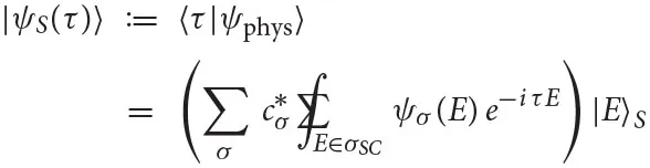^satisfies the same Schrödinger equation (40). However, it is straightforward to check, using Lemma 1, that these new clock states do not give rise to a resolution of the identity, ∫ dτ |τ〉 〈τ| ≠ I_C and so |ψ_phys〉 ≠ ∫ dτ |τ〉 |ψ_S(τ)〉. In fact, if c_σ ≠ 0 for σ = +, −, then |ψ_S(τ)〉 will mix contributions from the positive and negative frequency sectors such that it will become impossible to reconstruct (either of the positive or negative frequency part of) the physical state from it. That is, a reduction map 〈τ| ⊗ I_S, which only conditions on the clock time, would not be invertible. This is another consequence of the superselection rule discussed above which entails that superpositions and mixtures across σ-sectors are indistinguishable through Dirac observables. It is also another reason why we condition also on the frequency sector when defining the reduction map in Equation (38).

17. ^We put projection in quotation marks because it is not a true projection when applied to the physical Hilbert space as it only removes redundancy in the description, i.e., degrees of freedom which are fixed through the constraint. No physical information is lost, which is why this operation will be invertible. It would however be a projection on ${{H}}_{\text{kin}}$.

18. ^This is understood as appending the new clock tensor factor |p_t = −σϵ〉_C to the reduced system state $|{\psi }_S^{\sigma }\rangle$ and then applying the inverse of the trivialization (recall that the conditioning of physical states on clock readings is not a true projection and thus invertible, cf. previous footnote). Note that embedding the reduced system states back into the physical Hilbert space is a priori highly ambiguous since the system state alone no longer carries any information about the clock state which had been projected out. However, here it is the physical interpretation of the reduced state as being the description of the system S relative to the temporal reference system C that singles out the embedding into the clock-neutral (i.e., temporal-reference-system-neutral) ${{H}}_{\text{phys}}$. This physical interpretation is, of course, added information, but it is crucial. For a more detailed discussion of this topic, see Vanrietvelde et al. [71].

19. ^However, note that the quantization of this classical reduced phase space will in some cases, but not in general, coincide with the quantum theory on ${{H}}_{S,\sigma }^{\text{phys}}$ due to the generic inequivalence between Dirac and reduced quantization (see Supplementary Material).

20. ^Note that here we have a doubly degenerate system energy ${Ĥ}_S={\widehat{p}}^2+m^2$ in contrast to the expression in Equation (18) where we ignored degeneracy.

21. ^This also resolves the normalization issue appearing in Diaz et al. [50] where physical states were normalized using the kinematical, rather than physical inner product, thus yielding a divergent normalization (for equal mass states) in contrast to here.

22. ^It is instructive to see how this is linked to the (non-)covariance of the clock observable with respect to Ĉ_H. Let e_C be either the covariant e_C(τ) or non-covariant e_C(t). The denominator of Equation (37) reads

$\langle {\psi }_{\text{phys}}|e_C\otimes I_S{|{\psi }_{\text{phys}}\rangle }_{\text{kin}}=\langle {\psi }_{\text{kin}}|\delta ({\widehat{C}}_H)(e_C\otimes I_S){|{\psi }_{\text{phys}}\rangle }_{\text{kin}}.$

^Equation (44) implies that δ(Ĉ_H)(e_C(τ) ⊗ I_S) ≈ I_phys. This exploits the covariance and immediately shows that the denominator coincides with the physical inner product Equation (18). By contrast, the non-covariance entails δ(Ĉ_H)(e_C(t) ⊗ I_S) ≠ I_phys, so that in this case the denominator differs from the physical inner product.

23. ^The physical inner product for the positive frequency solutions ${\psi }_{\text{phys}}^{+}(t,x)$ to the Klein-Gordon equation takes, of course, the standard Klein-Gordon (and not the Schrödinger) form Equation (61). Nevertheless, the kernel K(x − x′) in the non-local convolution in the first line in Equation (65) decreases quickly as a function of m|x − x′| [90]. Hence, for massive particles, we can interpret even Equation (62) as providing an approximate localization.

24. ^Indeed, the Hamiltonian constraint of the vacuum Bianchi I and II models can be written in the form [116]

$\begin{array}{l}{\widehat{C}}_H=-\frac{{\widehat{\bar{p}}}_0^2}{2}+\frac{{\widehat{\bar{p}}}_{-}^2}{2}+\frac{{\widehat{\bar{p}}}_{+}^2}{2}+k_{+}{e}^{-4\sqrt{3}{\widehat{\bar{\beta }}}^{+}}.\end{array}$

25. ^Recall that the label “phys” highlights that the observable acts on the physical C₂S Hilbert space, i.e., on ${\Pi }_{{\sigma }_{C_{2}S{C}_1}}({{H}}_{C_2}\otimes {{H}}_S)$, where ${\Pi }_{{\sigma }_{C_{2}S{C}_1}}=\theta [-s_1(s_2\frac{{\widehat{p}}_2^2}{2}+{Ĥ}_S)]$ is the projector onto the subspace corresponding to the spectrum ${\sigma }_{C_{2}S{C}_1}≔\mathrm{\text{Spec}}\left(s_2\frac{{\widehat{p}}_2^2}{2}+{Ĥ}_S\right)\cap \mathrm{\text{Spec}}\left(-s_1\frac{{\widehat{p}}_1^2}{2}\right)$ permitted by the constraint Equation (66) (cf. Equation 17). We can thus also understand this observable as a projection ${Ô}_{C_{2}S|C_1}^{\text{phys}}≔{\Pi }_{{\sigma }_{C_{2}S{C}_1}}{Ô}_{C_{2}S|C_1}{\Pi }_{{\sigma }_{C_{2}S{C}_1}}$ of some observable ${Ô}_{C_{2}S|C_1}\in {L}({{H}}_{C_2}\otimes {{H}}_S)$; cf. Equation (36).

References

1. Kuchař KV. Time and interpretations of quantum gravity. Int J Mod Phys D. (2011) 20:3–86. doi: 10.1142/S0218271811019347

CrossRef Full Text | Google Scholar

2. Isham CJ. Canonical quantum gravity and the problem of time. In: Ibort LA, Rodríguez MA, editors. Integrable Systems, Quantum Groups, and Quantum Field Theories. Dordrecht: Springer Netherlands (1993). p. 157–287. doi: 10.1007/978-94-011-1980-1_6

PubMed Abstract | CrossRef Full Text | Google Scholar

3. Anderson E. The Problem of Time. Vol. 190 of Fundamental Theories of Physics. Basel: Springer International Publishing (2017).

Google Scholar

4. Rovelli C. Quantum Gravity. Cambridge: Cambridge University Press (2004).

Google Scholar

5. Smolin L. The Case for Background Independence. Oxford: Oxford University Press (2006).

Google Scholar

6. Smolin L. Temporal relationalism. arXiv. (2018) 180512468.

Google Scholar

7. Höhn PA, Smith ARH, Lock MPE. The trinity of relational quantum dynamics. arXiv. (2019) 191200033.

Google Scholar

8. DeWitt BS. Quantum theory of gravity. I. The canonical theory. Phys Rev. (1967) 160:1113–48. doi: 10.1103/PhysRev.160.1113

PubMed Abstract | CrossRef Full Text | Google Scholar

9. Rovelli C. Is there incompatibility between the ways time is treated in general relativity and in standard quantum mechanics. In: Ashtekar A, Stachel J, editors. Conceptual Problems of Quantum Gravity. Basel: Birkhauser (1991). p. 126–40.

Google Scholar

10. Ashtekar A. Lectures on Non-Perturbative Canonical Gravity. Vol. 6 of Physics and Cosmology. Singapore: World Scientific (1991).

Google Scholar

11. Thiemann T. Modern Canonical Quantum General Relativity. Cambridge: Cambridge University Press (2008).

Google Scholar

12. Rovelli C. Quantum mechanics without time: a model. Phys Rev D. (1990) 42:2638–46. doi: 10.1103/PhysRevD.42.2638

CrossRef Full Text | Google Scholar

13. Rovelli C. Time in quantum gravity: physics beyond the Schrödinger regime. Phys Rev D. (1991) 43:442–56. doi: 10.1103/PhysRevD.43.442

CrossRef Full Text | Google Scholar

14. Rovelli C. What is observable in classical and quantum gravity? Class Quantum Grav. (1991) 8:297–316. doi: 10.1088/0264-9381/8/2/011

CrossRef Full Text | Google Scholar

15. Rovelli C. Quantum reference systems. Class Quantum Grav. (1991) 8:317–32. doi: 10.1088/0264-9381/8/2/012

CrossRef Full Text | Google Scholar

16. Marolf D. Almost ideal clocks in quantum cosmology: a brief derivation of time. Class Quantum Grav. (1995) 12:2469–86. doi: 10.1088/0264-9381/12/10/007

CrossRef Full Text | Google Scholar

17. Marolf D. Quantum observables and recollapsing dynamics. Class Quantum Grav. (1995) 12:1199–220. doi: 10.1088/0264-9381/12/5/011

CrossRef Full Text | Google Scholar

18. Gambini R, Porto RA. Relational time in generally covariant quantum systems: four models. Phys Rev D. (2001) 63:105014. doi: 10.1103/PhysRevD.63.105014

CrossRef Full Text | Google Scholar

19. Tambornino J. Relational observables in gravity: a review. SIGMA. (2012) 8:017. doi: 10.3842/SIGMA.2012.017

CrossRef Full Text | Google Scholar

20. Giddings SB, Marolf D, Hartle JB. Observables in effective gravity. Phys Rev D. (2006) 74:064018. doi: 10.1103/PhysRevD.74.064018

CrossRef Full Text | Google Scholar

21. Dittrich B. Partial and complete observables for Hamiltonian constrained systems. Gen Relativ Gravit. (2007) 39:1891–927. doi: 10.1007/s10714-007-0495-2

CrossRef Full Text | Google Scholar

22. Dittrich B. Partial and complete observables for canonical general relativity. Class Quantum Grav. (2006) 23:6155–84. doi: 10.1088/0264-9381/23/22/006

CrossRef Full Text | Google Scholar

23. Dittrich B, Tambornino J. A perturbative approach to Dirac observables and their space-time algebra. Class Quantum Grav. (2007) 24:757–84. doi: 10.1088/0264-9381/24/4/001

CrossRef Full Text | Google Scholar

24. Dittrich B, Tambornino J. Gauge invariant perturbations around symmetry reduced sectors of general relativity: applications to cosmology. Class Quantum Grav. (2007) 24:4543–86. doi: 10.1088/0264-9381/24/18/001

CrossRef Full Text | Google Scholar

25. Gambini R, Porto RA, Pullin J, Torterolo S. Conditional probabilities with Dirac observables and the problem of time in quantum gravity. Phys Rev D. (2009) 79:041501. doi: 10.1103/PhysRevD.79.041501

CrossRef Full Text | Google Scholar

26. Pons JM, Salisbury DC, Sundermeyer KA. Revisiting observables in generally covariant theories in the light of gauge fixing methods. Phys Rev D. (2009) 80:084015. doi: 10.1103/PhysRevD.80.084015

CrossRef Full Text | Google Scholar

27. Ashtekar A, Pawlowski T, Singh P. Quantum nature of the big bang: an analytical and numerical investigation. I. Phys Rev D. (2006) 73:124038. doi: 10.1103/PhysRevD.73.124038

CrossRef Full Text | Google Scholar

28. Kaminski W, Lewandowski J, Pawlowski T. Physical time and other conceptual issues of QG on the example of LQC. Class Quantum Grav. (2009) 26:035012. doi: 10.1088/0264-9381/26/3/035012

CrossRef Full Text | Google Scholar

29. Kaminski W, Lewandowski J, Pawlowski T. Quantum constraints, Dirac observables and evolution: group averaging versus Schrodinger picture in LQC. Class Quantum Grav. (2009) 26:245016. doi: 10.1088/0264-9381/26/24/245016

CrossRef Full Text | Google Scholar

30. Höhn PA, Vanrietvelde A. How to switch between relational quantum clocks. New J Phys. (2020) 22:123048. doi: 10.1088/1367-2630/abd1ac

CrossRef Full Text | Google Scholar

31. Höhn PA. Switching internal times and a new perspective on the ‘wave function of the universe'. Universe. (2019) 5:116. doi: 10.3390/universe5050116

CrossRef Full Text | Google Scholar

32. Bojowald M, Höhn PA, Tsobanjan A. An effective approach to the problem of time. Class Quantum Grav. (2011) 28:035006. doi: 10.1088/0264-9381/28/3/035006

CrossRef Full Text | Google Scholar

33. Bojowald M, Höhn PA, Tsobanjan A. Effective approach to the problem of time: general features and examples. Phys Rev D. (2011) 83:125023. doi: 10.1103/PhysRevD.83.125023

CrossRef Full Text | Google Scholar

34. Höhn PA, Kubalova E, Tsobanjan A. Effective relational dynamics of a nonintegrable cosmological model. Phys Rev D. (2012) 86:065014. doi: 10.1103/PhysRevD.86.065014

CrossRef Full Text | Google Scholar

35. Dittrich B, Höhn PA, Koslowski TA, Nelson MI. Can chaos be observed in quantum gravity? Phys Lett B. (2017) 769:554–60. doi: 10.1016/j.physletb.2017.02.038

CrossRef Full Text | Google Scholar

36. Dittrich B, Höhn PA, Koslowski TA, Nelson MI. Chaos, Dirac observables and constraint quantization. arXiv. (2015) 150801947.

Google Scholar

37. Chataignier L. On the construction of quantum Dirac observables and the emergence of WKB time. Phys Rev D. (2020) 101:086001. doi: 10.1103/PhysRevD.101.086001

CrossRef Full Text | Google Scholar

38. Chataignier L. Relational observables, reference frames and conditional probabilities. arXiv. (2020) 200605526. doi: 10.1103/PhysRevD.103.026013

CrossRef Full Text | Google Scholar

39. Page DN, Wootters WK. Evolution without evolution: dynamics described by stationary observables. Phys Rev D. (1983) 27:2885. doi: 10.1103/PhysRevD.27.2885

CrossRef Full Text | Google Scholar

40. Wootters WK. “Time” replaced by quantum correlations. Int J Theor Phys. (1984) 23:701. doi: 10.1007/BF02214098

CrossRef Full Text | Google Scholar

41. Gambini R, Pullin J. Relational physics with real rods and clocks and the measurement problem of quantum mechanics. Found Phys. (2007) 37:1074–92. doi: 10.1007/s10701-007-9144-6

CrossRef Full Text | Google Scholar

42. Gambini R, Porto R, Pullin J. Fundamental decoherence from quantum gravity: a pedagogical review. Gen Relativ Gravit. (2007) 39:1143–56. doi: 10.1007/s10714-007-0451-1

CrossRef Full Text | Google Scholar

43. Giovannetti V, Lloyd S, Maccone L. Quantum time. Phys Rev D. (2015) 79:945933. doi: 10.1103/PhysRevD.92.045033

CrossRef Full Text | Google Scholar

44. Smith ARH, Ahmadi M. Quantizing time: interacting clocks and systems. Quantum. (2019) 3:160. doi: 10.22331/q-2019-07-08-160

CrossRef Full Text | Google Scholar

45. Smith ARH, Ahmadi M. Quantum clocks observe classical and quantum time dilation. Nat Commun. (2020) 11:5360. doi: 10.1038/s41467-020-18264-4

PubMed Abstract | CrossRef Full Text | Google Scholar

46. Dolby CE. The conditional probability interpretation of the Hamiltonian constraint. arXiv. (2004) 0406034.

Google Scholar

47. Castro-Ruiz E, Giacomini F, Belenchia A, Brukner Č. Quantum clocks and the temporal localisability of events in the presence of gravitating quantum systems. Nat Commun. (2020) 11:2672. doi: 10.1038/s41467-020-16013-1

PubMed Abstract | CrossRef Full Text | Google Scholar

48. Boette A, Rossignoli R. History states of systems and operators. Phys Rev A. (2018) 98:032108. doi: 10.1103/PhysRevA.98.032108

CrossRef Full Text | Google Scholar

49. Diaz NL, Rossignoli R. History state formalism for Dirac's theory. Phys Rev D. (2019) 99:045008. doi: 10.1103/PhysRevD.99.045008

CrossRef Full Text | Google Scholar

50. Diaz NL, Matera JM, Rossignoli R. History state formalism for scalar particles. Phys Rev D. (2019) 100:125020. doi: 10.1103/PhysRevD.100.125020

CrossRef Full Text | Google Scholar

51. Singh A. Quantum space, quantum time, and relativistic quantum mechanics. arXiv. (2020) 200409139.

Google Scholar

52. Leon J, Maccone L. The Pauli objection. Found Phys. (2017) 47:1597–608. doi: 10.1007/s10701-017-0115-2

CrossRef Full Text | Google Scholar

53. Marletto C, Vedral V. Evolution without evolution and without ambiguities. Phys Rev D. (2017) 95:043510. doi: 10.1103/PhysRevD.95.043510

CrossRef Full Text | Google Scholar

54. Nikolova A, Brennen G, Osborne TJ, Milburn G, Stace TM. Relational time in anyonic systems. Phys Rev A. (2018) 97:030101. doi: 10.1103/PhysRevA.97.030101

CrossRef Full Text | Google Scholar

55. Baumann V, Santo FD, Smith ARH, Giacomini F, Castro-Ruiz E, Brukner C. Generalized probability rules from a timeless formulation of Wigner's friend scenarios. arXiv. (2019) 191109696.

Google Scholar

56. Favalli T, Smerzi A. Hermitian time operator in a timeless universe. arXiv. (2020) 200309042. doi: 10.22331/q-2020-10-29-354

CrossRef Full Text | Google Scholar

57. Foti C, Coppo A, Barni G, Cuccoli A, Verrucchi P. There is only one time. arXiv. (2020) 200612103.

Google Scholar

58. Thiemann T. Reduced phase space quantization and Dirac observables. Class Quantum Grav. (2006) 23:1163–80. doi: 10.1088/0264-9381/23/4/006

CrossRef Full Text | Google Scholar

59. Bojowald M, Tsobanjan A. Quantization of dynamical symplectic reduction. arXiv. (2019) 190604792. doi: 10.1007/s00220-020-03856-4

CrossRef Full Text | Google Scholar

60. Giesel K, Thiemann T. Algebraic quantum gravity (AQG). IV. Reduced phase space quantisation of loop quantum gravity. Class Quantum Grav. (2010) 27:175009. doi: 10.1088/0264-9381/27/17/175009

CrossRef Full Text | Google Scholar

61. Domagala M, Giesel K, Kaminski W, Lewandowski J. Gravity quantized: loop quantum gravity with a scalar field. Phys Rev D. (2010) 82:104038. doi: 10.1103/PhysRevD.82.104038

CrossRef Full Text | Google Scholar

62. Husain V, Pawlowski T. Time and a physical Hamiltonian for quantum gravity. Phys Rev Lett. (2012) 108:141301. doi: 10.1103/PhysRevLett.108.141301

PubMed Abstract | CrossRef Full Text | Google Scholar

63. Giesel K, Vetter A. Reduced loop quantization with four Klein-Gordon scalar fields as reference matter. Class Quantum Grav. (2019) 36:145002. doi: 10.1088/1361-6382/ab26f4

CrossRef Full Text | Google Scholar

64. Giesel K, Herold L, Li BF, Singh P. Mukhanov-Sasaki equation in manifestly gauge-invariant linearized cosmological perturbation theory with dust reference fields. Phys Rev D. (2020) 102:023524. doi: 10.1103/PhysRevD.102.023524

CrossRef Full Text | Google Scholar

65. Giesel K, Li BF, Singh P. Towards a reduced phase space quantization in loop quantum cosmology with an inflationary potential. arXiv. (2020) 200706597. doi: 10.1103/PhysRevD.102.126024

CrossRef Full Text | Google Scholar

66. Albrecht A, Iglesias A. The clock ambiguity and the emergence of physical laws. Phys Rev D. (2008) 77:063506. doi: 10.1103/PhysRevD.77.063506

CrossRef Full Text | Google Scholar

67. Albrecht A, Iglesias A. The clock ambiguity: implications and new developments. In: Mersini-Houghton L, Vaas R, editors. The Arrows of Time. Fundamental Theories of Physics, Vol. 172. Berlin; Heidelberg: Springer (2012). doi: 10.1007/978-3-642-23259-6_4

CrossRef Full Text | Google Scholar

68. Corbin V, Cornish NJ. Semi-classical limit and minimum decoherence in the conditional probability interpretation of quantum mechanics. Found Phys. (2009) 39:474. doi: 10.1007/s10701-009-9298-5

CrossRef Full Text | Google Scholar

69. Bojowald M, Halnon T. Time in quantum cosmology. Phys Rev D. (2018) 98:066001. doi: 10.1103/PhysRevD.98.066001

CrossRef Full Text | Google Scholar

70. Giacomini F, Castro-Ruiz E, Brukner Č. Quantum mechanics and the covariance of physical laws in quantum reference frames. Nat Commun. (2019) 10:494. doi: 10.1038/s41467-018-08155-0

PubMed Abstract | CrossRef Full Text | Google Scholar

71. Vanrietvelde A, Höhn PA, Giacomini F, Castro-Ruiz E. A change of perspective: switching quantum reference frames via a perspective-neutral framework. Quantum. (2020) 4:225. doi: 10.22331/q-2020-01-27-225

CrossRef Full Text | Google Scholar

72. Vanrietvelde A, Höhn PA, Giacomini F. Switching quantum reference frames in the N-body problem and the absence of global relational perspectives. arXiv. (2018) 180905093.

Google Scholar

73. Giacomini F, Castro-Ruiz E, Brukner Č. Relativistic quantum reference frames: the operational meaning of spin. Phys Rev Lett. (2019) 123:090404. doi: 10.1103/PhysRevLett.123.090404

PubMed Abstract | CrossRef Full Text | Google Scholar

74. de la Hamette AC, Galley TD. Quantum reference frames for general symmetry groups. Quantum. (2020) 4:367. doi: 10.22331/q-2020-11-30-367

CrossRef Full Text | Google Scholar

75. Loveridge L, Miyadera T, Busch P. Symmetry, reference frames, and relational quantities in quantum mechanics. Found Phys. (2018) 48:135–98. doi: 10.1007/s10701-018-0138-3

CrossRef Full Text | Google Scholar

76. Yang JM. Switching quantum reference frames for quantum measurement. Quantum. (2020) 4:283. doi: 10.22331/q-2020-06-18-283

CrossRef Full Text | Google Scholar

77. Gielen S, Menéndez-Pidal L. Singularity resolution depends on the clock. arXiv. (2020) 200505357. doi: 10.1088/1361-6382/abb14f

CrossRef Full Text | Google Scholar

78. Savi MF, Angelo RM. Quantum resources covariance. arXiv. (2020) 200509612. doi: 10.1103/PhysRevA.103.022220

CrossRef Full Text | Google Scholar

79. Le TP, Mironowicz P, Horodecki P. Blurred quantum Darwinism across quantum reference frames. arXiv. (2020) 200606364. doi: 10.1103/PhysRevA.102.062420

CrossRef Full Text | Google Scholar

80. Tuziemski J. Decoherence and information encoding in quantum reference frames. arXiv. (2020) 200607298.

Google Scholar

81. Hardy L. The construction interpretation: conceptual roads to quantum gravity. arXiv. (2018) 180710980.

Google Scholar

82. Hardy L. Implementation of the quantum equivalence principle. In: Finster F, Giulini D, Kleiner J, Tolksdorf J, editors. Progress and Visions in Quantum Theory in View of Gravity: Bridging Foundations of Physics and Mathematics. Basel: Birkhäuser (2020). p. 189–220. doi: 10.1007/978-3-030-38941-3_8

CrossRef Full Text | Google Scholar

83. Guérin PA, Brukner Č. Observer-dependent locality of quantum events. New J Phys. (2018) 20:103031. doi: 10.1088/1367-2630/aae742

CrossRef Full Text | Google Scholar

84. Zych M, Costa F, Ralph TC. Relativity of quantum superpositions. arXiv. (2018) 180904999.

Google Scholar

85. Barbado LC, Castro-Ruiz E, Apadula L, Brukner Č. Unruh effect for detectors in superposition of accelerations. arXiv. (2020) 200312603. doi: 10.1103/PhysRevD.102.045002

CrossRef Full Text | Google Scholar

86. Holevo AS. Probabilistic and Statistical Aspects of Quantum Theory. Vol. 1 of Statistics and Probability. Amsterdam: North-Holland Publishing Company (1982).

Google Scholar

87. Busch P, Grabowski M, Lahti PJ. Operational Quantum Physics. Vol. 31 of Lecture Notes in Physics Monographs. Berlin; Heidelberg: Springer-Verlag (1995).

Google Scholar

88. Busch P, Grabowski M, Lahti PJ. Time observables in quantum theory. Phys Lett A. (1994) 191:357–61. doi: 10.1016/0375-9601(94)90785-4

CrossRef Full Text | Google Scholar

89. Braunstein SL, Caves CM, Milburn GJ. Generalized uncertainty relations: theory, examples, and Lorentz invariance. Ann Phys. (1996) 247:135–73. doi: 10.1006/aphy.1996.0040

CrossRef Full Text | Google Scholar

90. Haag R. Local Quantum Physics: Fields, Particles, Algebras. Berlin; Heidelberg: Springer-Verlag (2012).

Google Scholar

91. Newton TD, Wigner EP. Localized states for elementary systems. Rev Mod Phys. (1949) 21:400–6. doi: 10.1103/RevModPhys.21.400

CrossRef Full Text | Google Scholar

92. Fernando Perez J, Wilde IF. Localization and causality in relativistic quantum mechanics. Phys Rev D. (1977) 16:315. doi: 10.1103/PhysRevD.16.315

CrossRef Full Text | Google Scholar

93. Malament DB. In defense of dogma: why there cannot be a relativistic quantum mechanics of (Localizable) particles. In: Clifton R, editor. Perspectives on Quantum Reality. The University of Western Ontario Series in Philosophy of Science (A Series of Books in Philosophy of Science, Methodology, Epistemology, Logic, History of Science, and Related Fields), Vol. 57. Dordrecht: Springer (1996). p. 1–10. doi: 10.1007/978-94-015-8656-6_1

CrossRef Full Text | Google Scholar

94. Yngvason J. Localization and entanglement in relativistic quantum physics. Lect Notes Phys. (2015) 899:325–48. doi: 10.1007/978-3-662-46422-9_15

CrossRef Full Text | Google Scholar

95. Papageorgiou M, Pye J. Impact of relativity on particle localizability and ground state entanglement. J Phys A. (2019) 52:375304. doi: 10.1088/1751-8121/ab3593

CrossRef Full Text | Google Scholar

96. Brunetti R, Fredenhagen K, Hoge M. Time in quantum physics: from an external parameter to an intrinsic observable. Found Phys. (2010) 40:1368–78. doi: 10.1007/s10701-009-9400-z

CrossRef Full Text | Google Scholar

97. Loveridge L, Miyadera T. Relative quantum time. Found Phys. (2019) 49:549–60. doi: 10.1007/s10701-019-00268-w

CrossRef Full Text | Google Scholar

98. Höhn PA. Reflections on the information paradigm in quantum and gravitational physics. J Phys Conf Ser. (2017) 880:012014. doi: 10.1088/1742-6596/880/1/012014

CrossRef Full Text | Google Scholar

99. Dalla Chiara ML. Logical self reference, set theoretical paradoxes and the measurement problem in quantum mechanics. J Philos Logic. (1977) 6:331–47. doi: 10.1007/BF00262066

CrossRef Full Text | Google Scholar

100. Breuer T. The impossibility of accurate state self-measurements. Philos Sci. (1995) 62:197–214. doi: 10.1086/289852

CrossRef Full Text | Google Scholar

101. Dirac PAM. Lectures on Quantum Mechanics. New York, NY: Belfer Graduate School of Sciencem Yeshiva University (1964).

Google Scholar

102. Henneaux M, Teitelboim C. Quantization of Gauge Systems. Princeton, NJ: Princeton University Press (1992).

Google Scholar

103. Marolf D. Refined algebraic quantization: systems with a single constraint. arXiv. (1995) 9508015.

Google Scholar

104. Hartle JB, Marolf D. Comparing formulations of generalized quantum mechanics for reparametrization–invariant systems. Phys Rev D. (1997) 56:6247–57. doi: 10.1103/PhysRevD.56.6247

CrossRef Full Text | Google Scholar

105. Giulini D, Marolf D. On the generality of refined algebraic quantization. Class Quantum Grav. (1999) 16:2479–88. doi: 10.1088/0264-9381/16/7/321

CrossRef Full Text | Google Scholar

106. Giulini D, Marolf D. A Uniqueness theorem for constraint quantization. Class Quantum Grav. (1999) 16:2489–505. doi: 10.1088/0264-9381/16/7/322

CrossRef Full Text | Google Scholar

107. Marolf D. Group averaging and refined algebraic quantization: where are we now? arXiv. (2000) 0011112.

Google Scholar

108. Pailas T. “Time”-covariant Schrödinger equation and the canonical quantization of the Reissner-Nordström black hole. arXiv. (2020). doi: 10.3390/quantum2030029

CrossRef Full Text | Google Scholar

109. Blyth WF, Isham CJ. Quantization of a Friedmann universe filled with a scalar field. Phys Rev D. (1975) 11:768–78. doi: 10.1103/PhysRevD.11.768

CrossRef Full Text | Google Scholar

110. Hawking SW. Quantum cosmology. In: DeWitt BS, Stora R, editors. Relativity, Groups and Topology II, Les Houches Summer School, 1983. Amsterdam: North-Holland Publishing Company (1984). p. 333.

Google Scholar

111. Hájíček P. Origin of nonunitarity in quantum gravity. Phys Rev D. (1986) 34:1040. doi: 10.1103/PhysRevD.34.1040

CrossRef Full Text | Google Scholar

112. Kiefer C. Wave packets in minisuperspace. Phys Rev D. (1988) 38:1761. doi: 10.1103/PhysRevD.38.1761

CrossRef Full Text | Google Scholar

113. Ashtekar A, Singh P. Loop quantum cosmology: a status report. Class Quantum Grav. (2011) 28:213001. doi: 10.1088/0264-9381/28/21/213001

CrossRef Full Text | Google Scholar

114. Ashtekar A, Corichi A, Singh P. Robustness of key features of loop quantum cosmology. Phys Rev D. (2008) 77:024046. doi: 10.1103/PhysRevD.77.024046

CrossRef Full Text | Google Scholar

115. Bojowald M. Canonical Gravity and Applications: Cosmology, Black Holes and Quantum Gravity. Cambridge: Cambridge University Press (2010).

Google Scholar

116. Ashtekar A, Tate R, Uggla C. Minisuperspaces: observables and quantization. Int J Mod Phys D. (1993) 2:15–50. doi: 10.1142/S0218271893000039

CrossRef Full Text | Google Scholar

117. Grot N, Rovelli C, Tate RS. Time-of-arrival in quantum mechanics. Phys Rev A. (1996) 54:4676. doi: 10.1103/PhysRevA.54.4676

CrossRef Full Text | Google Scholar

118. Aharonov Y, Oppenheim J, Popescu S, Reznik B, Unruh W. Measurement of time of arrival in quantum mechanics. Phys Rev A. (1998) 57:4130. doi: 10.1103/PhysRevA.57.4130

CrossRef Full Text | Google Scholar

119. Muga JG, Leavens CR. Arrival time in quantum mechanics. Phys Rep. (2000) 338:353–438. doi: 10.1016/S0370-1573(00)00047-8

CrossRef Full Text | Google Scholar

120. Aharonov Y, Bohm D. Time in the quantum theory and the uncertainty relation for time and energy. Phys Rev. (1961) 122:1649. doi: 10.1103/PhysRev.122.1649

CrossRef Full Text | Google Scholar

121. Peres A. Measurement of time by quantum clocks. Am J Phys. (1980) 48:552–7. doi: 10.1119/1.12061

CrossRef Full Text | Google Scholar

122. Pauli W. Die allgemeinen prinzipien der wellenmechanik. Handbuch der Physik. (1958) 5:1–168. doi: 10.1007/978-3-642-80539-4_1

CrossRef Full Text | Google Scholar

123. Rovelli C. Partial observables. Phys Rev D. (2002) 65:124013. doi: 10.1103/PhysRevD.65.124013

CrossRef Full Text | Google Scholar

124. Ashtekar A, Horowitz G. On the canonical approach to quantum gravity. Phys Rev D. (1982) 26:3342–53. doi: 10.1103/PhysRevD.26.3342

CrossRef Full Text | Google Scholar

125. Kuchař KV. Covariant factor ordering of gauge systems. Phys Rev D. (1986) 34:3044–57. doi: 10.1103/PhysRevD.34.3044

PubMed Abstract | CrossRef Full Text | Google Scholar

126. Schleich K. Is reduced phase space quantization equivalent to Dirac quantization? Class Quantum Grav. (1990) 7:1529–38. doi: 10.1088/0264-9381/7/8/028

CrossRef Full Text | Google Scholar

127. Romano JD, Tate RS. Dirac versus reduced space quantization of simple constrained systems. Class Quantum Grav. (1989) 6:1487. doi: 10.1088/0264-9381/6/10/017

CrossRef Full Text | Google Scholar

128. Loll R. Noncommutativity of constraining and quantizing: a U(1) gauge model. Phys Rev D. (1990) 41:3785–91. doi: 10.1103/PhysRevD.41.3785

PubMed Abstract | CrossRef Full Text | Google Scholar

129. Kunstatter G. Dirac versus reduced quantization: a geometrical approach. Class Quantum Grav. (1992) 9:1469–86. doi: 10.1088/0264-9381/9/6/005

CrossRef Full Text | Google Scholar

130. Bartlett SD, Rudolph T, Spekkens RW. Reference frames, superselection rules, and quantum information. Rev Mod Phys. (2007) 79:555–609. doi: 10.1103/RevModPhys.79.555

CrossRef Full Text | Google Scholar

131. Smith ARH. Communicating without shared reference frames. Phys Rev A. (2019) 99:052315. doi: 10.1103/PhysRevA.99.052315

CrossRef Full Text | Google Scholar

132. Smith ARH, Piani M, Mann RB. Quantum reference frames associated with noncompact groups: the case of translations and boosts and the role of mass. Phys Rev A. (2016) 94:012333. doi: 10.1103/PhysRevA.94.012333

CrossRef Full Text | Google Scholar

133. Banerjee K, Calcagni G, Martín-Benito M. Introduction to loop quantum cosmology. SIGMA. (2012) 8:016. doi: 10.3842/SIGMA.2012.016

CrossRef Full Text | Google Scholar

134. Page DN. Time as an Inaccessible Observable. NSF-ITP-89-18 (1989).

Google Scholar

135. Page DN. Clock time and entropy. In: Halliwell JJ, Pérez-Mercader J, Zurek WH, editors. Physical Origins of Time Asymmetry. Cambridge: Cambridge University Press (1994). p. 287–98.

Google Scholar

136. Smith ARH. Quantum time dilation: a new test of relativistic quantum theory. arXiv. (2020) 200410810.

Google Scholar

137. Grochowski PT, Smith ARH, Dragan A, Dȩbski K. Quantum time dilation in atomic spectra. Physic Rev Res. (2021) 3:023053. doi: 10.1103/PhysRevResearch.3.023053

CrossRef Full Text | Google Scholar

138. Zych M, Costa F, Pikovski I, Brukner Č. Quantum interferometric visibility as a witness of general relativistic proper time. Nat Commun. (2011) 2:505. doi: 10.1038/ncomms1498

PubMed Abstract | CrossRef Full Text | Google Scholar

139. Khandelwal S, Lock MPE, Woods MP. Universal quantum modifications to general relativistic time dilation in delocalised clocks. Quantum. (2020) 4:309. doi: 10.22331/q-2020-08-14-309

CrossRef Full Text | Google Scholar

140. Paige AJ, Plato ADK, Kim MS. Classical and nonclassical time dilation for quantum clocks. Phys Rev Lett. (2020) 124:160602. doi: 10.1103/PhysRevLett.124.160602

PubMed Abstract | CrossRef Full Text | Google Scholar