Training Restricted Boltzmann Machines With a D-Wave Quantum Annealer

1 Introduction

Quantum computing holds promise for a revolution in the field of science, engineering, and industry. Most of the R&D work related to quantum computing is focused on gate based approach [1–3], an alternative to this is the adiabatic quantum computing (AQC) [4–7]. In AQC, a system of qubits starts with a simple Hamiltonian whose ground state is known. Gradually, the initial Hamiltonian evolves into a final Hamiltonian. The final Hamiltonian is designed in such a way that its ground state corresponds to the solution to the problem of interest. According to the quantum adiabatic theorem, a quantum system that begins in the non-degenerate ground state of a time-dependent Hamiltonian will remain in the instantaneous ground state provided the Hamiltonian changes sufficiently slowly [8–11]. It has been shown theoretically that an AQC machine can give solutions that are very difficult to find using classical methods [12].

D-Wave’s quantum annealer has been investigated by several researchers for machine learning and optimization problems. Mott et al. [13] used D-Wave to classify Higgs-boson-decay signals vs. background. They showed that the quantum annealing-based classifiers perform comparably to the state-of-the-art machine learning methods. Das et al. has used a D-Wave for clustering applications [14]. Mniszewski et al. [15] found that the results for graph partitioning using D-Wave systems are comparable to commonly used methods. Alexandrov et al. [16] used a D-Wave for matrix factorization. Lidar et al. [17] used a D-Wave for the classification of DNA sequences according to their binding affinities. Kais et al. have used D-Wave’s quantum annealer for prime factorization and electronic structure calculation of molecular systems [18, 19].

RBM is a widely used machine learning technique for unsupervised and supervised tasks. However, its training is time consuming due to the calculation of model-dependent term in gradient learning. RBMs are usually trained using a method known as Contrastive Divergence (CD). CD uses Markov chain Monte Carlo (MCMC) which requires a long equilibration time. Further, the CD does not follow the gradient of the log-likelihood [20] and is not guaranteed to give correct results. Therefore, better sampling methods can have a positive impact on RBM learning. Among other works related to the topic, Adachi et al. [21] used quantum annealing for training RBMs, which were further used as layers of a two-layered deep neural network and post-trained by the back-propagation algorithm. The authors conclude that the hybrid approach results in faster training, although the relative effectiveness of RBM trained using a quantum-annealer vs. contrastive divergence has not been documented. Benedetti et al. [22] used a D-Wave quantum annealer to train an RBM on a 16-bit bars and stripes dataset. To train the RBM effectively an instance dependent temperature was calculated during each iteration. Caldeira et al. [23] used a QA-trained RBM for galaxy morphology image classification. Principal component analysis was used to compress the original dataset. They also explored the use of temperature estimation and examined the effect of noise by comparing the results from an older machine and a newer lower-noise version. Sleeman et al. [24] investigated a hybrid system that combined a classical deep neural network autoencoder with a QA-based RBM. Two datasets, the MNIST and the MNIST Fashion datasets, were used in this study. Image classification and image reconstruction were investigated. Winci et al. [25] developed a quantum-classical hybrid algorithm for a variational autoencoder (VAE). A D-Wave quantum annealer was used as a Boltzmann sampler for training the VAE. Dymtro et al. [26] performed a benchmarking study, to show that for harder problems Boltzmann machines trained using quantum annealing gives better gradients as compared to CD. Lorenzo et al. [27] used RBM trained with reverse annealing to carry out semantic learning that achieved good scores on reconstruction tasks. Koshka et al. [28] showed D-Wave quantum annealing performed better than classical simulated annealing for RBM training when the number of local valleys on the energy landscape was large. Dumoulin et al. [29] assessed the effect of various parameters like limited connectivity, and noise in weights and biases of RBM on its performance. Koshka et al. explored the energy landscape of an RBM embedded onto a D-Wave machine, which was trained with CD [30–33]. Dixit et al. [34] used a QA-trained RBM to balance the ISCX cybersecurity dataset, and training an intrusion detection classifier. There has been growing interest in quantum machine learning including Boltzmann machines [35–38], however, training quantum machine learning models on a moderate or large dataset is challenging. An RBM with 64 visible and 64 hidden units can be trained using a quantum annealer which is very difficult to do using existing gate based approaches.

In this work, our objective is to train an RBM using quantum annealing (QA) via samples obtained from the D-Wave 2000Q quantum annealer and compare its performance with an RBM trained with CD. The model-dependent term in the gradient of log-likelihood has been estimated by using samples drawn from a quantum annealer. Trained models are compared with respect to classification accuracy, image reconstruction, and log-likelihood values. To carry out this study, the bars and stripes (BAS) dataset has been used.

2 Methods

2.1 Restricted Boltzmann Machine

A Restricted Boltzmann Machine is an energy-based model, inspired by the Boltzmann distribution of energies for the Ising model of spins. An RBM models the underlying probability distribution of a dataset and can be used for machine learning applications. However, an efficient method of RBM training is still not discovered. An RBM is comprised of two layers of binary variables known as visible and hidden layers. The variables or units in the visible and hidden layers are denoted as $\left\{v_1,v_2,\dots .,v_n\right\}$ and $\left\{h_1,h_2,\dots .,h_m\right\}$, respectively. The variables in one layer interact with the variables in the other layer, however, interactions between the variables in the same layer are not permitted. The energy of the model is given by:

$E=-{\displaystyle \sum }_i{b}_i{v}_i-{\displaystyle \sum }_j{c}_j{h}_j-{\displaystyle \sum }_{i,j}{v}_i{w}_{ij}{h}_j,(1)$

where $b_i$ and $c_j$ are bias terms; $w_{ij}$ represents the strength of the interaction between variables $v_i$ and $h_j$. Let us represent the variables in the visible layer collectively by a vector: $v\in {\left\{\mathrm{0,1}\right\}}^n$, similarly for the hidden layer: $h\in {\left\{\mathrm{0,1}\right\}}^m$. Using this representation Eq. 1 can be written as:

$E\left(v,h\right)=-b^{T}v-c^{T}h-h^{T}Wv,(2)$

where b and c are bias vectors at the visible and hidden layer, respectively; W is a weight matrix composed of $w_{ij}$ elements. The probability that the model assigns to the configuration $\left\{v,h\right\}$ is:

$P\left(v,h\right)=\frac{1}{Z}{e}^{-E\left(v,h\right)},Z={\displaystyle \sum }_v{\displaystyle \sum }_h{e}^{-E\left(v,h\right)},(3)$

where Z is the partition function. Substituting value of $E\left(v,h\right)$, from Eq. 2, we get:

$Z={\displaystyle \sum }_v{\displaystyle \sum }_h{e}^{b^{T}v+c^{T}h+h^T\cdot W\cdot v}={\displaystyle \sum }_h{e}^{c^{T}h}{\displaystyle \sum }_v{e}^{b^{T}v+h^T\cdot W\cdot v}(4)$

$Z={\displaystyle \sum }_h{e}^{c^{T}h}{\displaystyle \sum }_v{e}^{\left(b^T+h^T\cdot W\right)v}={\displaystyle \sum }_h{e}^{c^{T}h}{\displaystyle \sum }_v{e}^{s\cdot v},(5)$

where s is:

$s=b^T+h^{T}W=\left[s_1,s_2,\dots ,s_n\right];(6)$

n is the number of variables in the visible layer. Now, Z can be written as:

$Z={\displaystyle \sum }_h{e}^{c^{T}h}{\displaystyle \prod }_{j=1}^n\left(1+e^{s_j}\right)(7)$

From Eq. 7, we notice that the calculation of Z involves summation over $2^m$ configuration, where m is the number of variables in the hidden layer. On the contrary, we need $2^{m+n}$ configurations to evaluate Z using Eq. 3.

2.2 Maximization of the Log-likelihood Cost Function

The partition function, Z, is hard to evaluate. The joint probability, $P\left(v,h\right)$, being a function of Z is also hard. Due to the bipartite graph structure of the RBM, the conditional distributions $P\left(h|v\right)$ and $P\left(v|h\right)$ are simple to compute,

$P\left(h|v\right)=\frac{P\left(v,h\right)}{P\left(v\right)}(8)$

where $P\left(v\right)$ is given by the following expression:

$P\left(v\right)=\frac{{{\displaystyle \sum }}_h{e}^{-E\left(v,h\right)}}{Z}.(9)$

Substituting values from Eq. 3 and Eq. 9 into Eq. 8 gives:

$P\left(h|v\right)=\frac{exp\left\{{{\displaystyle \sum }}_j{c}_j{h}_j+{{\displaystyle \sum }}_j{\left(v^{T}W\right)}_j{h}_j\right\}}{Z\prime },(10)$

where

$Z^{\prime }={\displaystyle \sum }_{h}exp\left(c^{T}h+h^{T}Wv\right).(11)$

$P\left(h|v\right)=\frac{1}{Z^{\prime }}{\displaystyle \prod }_{j}exp\left\{c_j{h}_j+{\left(v^{T}W\right)}_j{h}_j\right\}(12)$

Let’s denote

$\tilde{P}\left(h_j|v\right)=exp\left\{c_j{h}_j+{\left(v^{T}W\right)}_j{h}_j\right\}(13)$

Now, the probability to find an individual variable in the hidden layer $h_j=1$ is:

$P\left(h_j=1|v\right)=\frac{\tilde{P}\left(h_j=1|v\right)}{\tilde{P}\left(h_j=0|v\right)+\tilde{P}\left(h_j=1|v\right)}=\frac{exp\left\{c_j+{\left(v^{T}W\right)}_j\right\}}{1+exp\left\{c_j+{\left(v^{T}W\right)}_j\right\}}(14)$

Thus, the individual hidden activation probability is given by:

$P\left(h_j=1|v\right)=\sigma \left(c_j+{\left(v^{T}W\right)}_j\right),(15)$

Where σ is the logistic function. Similarly, the activation probability of a visible variable conditioned on a hidden vector h is given by:

$P\left(v_i=1|h\right)=\sigma \left(b_i+{\left(h^{T}W\right)}_i\right).(16)$

An RBM is trained by maximizing the likelihood of the training data. The log-likelihood is given by:

$l\left(W,b,c\right)={\displaystyle \sum }_{t=1}^N\text{log}P\left(v^{\left(t\right)}\right)={\displaystyle \sum }_{t=1}^N\text{log}{\displaystyle \sum }_{h}P\left(v^{\left(t\right)},h\right)(17)$

$l\left(W,b,c\right)={\displaystyle \sum }_{t=1}^N\text{log}{\displaystyle \sum }_h{e}^{-E\left(v^{\left(t\right)},h\right)}-N\cdot \text{log}{\displaystyle \sum }_{v,h}{e}^{-E\left(v,h\right)}.(18)$

Where $v^{\left(t\right)}$ is a sample from the training dataset. Denote $\theta =\left\{W,b,c\right\}$. The gradient of the log-likelihood is given by:

${\nabla }_{\theta }l\left(\theta \right)={\displaystyle \sum }_{t=1}^N\frac{{{\displaystyle \sum }}_h{e}^{-E\left(v^{\left(t\right)},h\right)}{\nabla }_{\theta }\left(-E\left(v^{\left(t\right)},h\right)\right)}{{{\displaystyle \sum }}_h{e}^{-E\left(v^{\left(t\right)},h\right)}}-N\cdot \frac{{{\displaystyle \sum }}_{v,h}{e}^{-E\left(v,h\right)}{\nabla }_{\theta }\left(-E\left(v,h\right)\right)}{{{\displaystyle \sum }}_{v,h}{e}^{-E\left(v,h\right)}}(19)$

${\nabla }_{\theta }l\left(\theta \right)={\displaystyle \sum }_{t=1}^N{\langle {\nabla }_{\theta }\left(-E\left(v^{\left(t\right)},h\right)\right)\rangle }_{P\left(h|v^{\left(t\right)}\right)}-N\cdot {\langle {\nabla }_{\theta }\left(-E\left(v,h\right)\right)\rangle }_{P\left(v,h\right)},(20)$

Where ${\langle \cdot \rangle }_{P\left(v,h\right)}$ is the expectation value with respect to the distribution $P\left(v,h\right)$. The gradient with respect to θ can also be expressed in terms of its components:

${\nabla }_{w}l=\frac{1}{N}{\displaystyle \sum }_{t=1}^N{\langle v^{\left(t\right)}\cdot h^{\left(t\right)}\rangle }_{P\left(h|v^{\left(t\right)}\right)}-{\langle v\cdot h\rangle }_{P\left(v,h\right)}(21)$

${\nabla }_{b}l=\frac{1}{N}{\displaystyle \sum }_{t=1}^N{\langle v^{\left(t\right)}\rangle }_{P\left(h|v^{\left(t\right)}\right)}-{\langle v\rangle }_{P\left(v,h\right)}(22)$

${\nabla }_{c}l=\frac{1}{N}{\displaystyle \sum }_{t=1}^N{\langle h^{\left(t\right)}\rangle }_{P\left(h|v^{\left(t\right)}\right)}-{\langle h\rangle }_{P\left(v,h\right)}(23)$

The first term in Eq. 20 is the expectation value of ${\nabla }_{\theta }\left(-E\left(v^{\left(t\right)},h\right)\right)$ with respect to the Boltzmann distribution, $v^{\left(t\right)}$ is a row vector from the training dataset with N records, and h is a hidden vector. Given $v^{\left(t\right)}$, h can be calculated via Eq. 15.

The second term in Eq. 20 is a model-dependent term, the expectation value of ${\nabla }_{\theta }\left(-E\left(v,h\right)\right)$, v and h can be any possible binary vectors. This term is difficult to evaluate as it requires all possible combinations of v and h. Generally, this term is estimated using contrastive divergence, where one uses many cycles of Gibbs sampling to transform the training data into data drawn from the proposed distribution. We used Eq. 15 and Eq. 16 to sample from hidden and visible layers repeatedly. Once we have the gradient of log-likelihood (Eq. 18), weights and biases can be estimated using gradient ascent optimization:

${\theta }_j^{new}={\theta }_j^{old}+\mathit{ϵ}\cdot {\nabla }_{{\theta }_j}l\left({\theta }_j\right)(24)$

where $\mathit{ϵ}$ is the learning rate.

Alternatively, the second term can be calculated using samples drawn from the D-Wave quantum annealer, which is a faster procedure than MCMC.

2.3 D-Wave Hamiltonian and Arrangement of Qubits

The Hamiltonian for a D-Wave system of qubits can be represented as:

$h_{Ising}=-\frac{A\left(s\right)}{2}\left({\displaystyle \sum }_i{\widehat{\sigma }}_x^i\right)+\frac{B\left(s\right)}{2}\left({\displaystyle \sum }_i{h}_i{\widehat{\sigma }}_z^i+{\displaystyle \sum }_{(i>j)}{J}_{ij}{\widehat{\sigma }}_z^i{\widehat{\sigma }}_z^j\right)(25)$

where ${\widehat{\sigma }}_{x,z}^{\left(i\right)}$ are Pauli matrices operating on $i^{th}$ qubit. $h_i$ and $J_{ij}$ are the qubit biases and coupling strengths. s is called the anneal fraction. $A\left(s\right)$ and $B\left(s\right)$ are known as anneal functions. At $s=0$, $A\left(s\right)\gg B\left(s\right)$, while $A\left(s\right)\ll B\left(s\right)$ for $s=1$. As we increase s from 0 to 1, anneal functions change gradually to meet these boundary conditions. In the standard quantum annealing (QA) protocol, s changes from 0 to 1. The network of qubits starts in a global superposition over all possible classical states and after $s=1$, the system is measured in a single classical state.

The arrangement of qubits on the D-Wave 2000Q quantum annealer forms a C16 Chimera graph with $16\times 16$ unit cells (2048 qubits are mapped into $16\times 16$ matrices of unit cells; each unit cell has eight qubits). Figure 1A shows a C3 Chimera graph with $3\times 3$ unit cells. Within each unit cell, there are two sets of four qubits that are connected in a bipartite fashion. As shown in the figure, each qubit in a unit cell is connected to four qubits of the same unit cell and two qubits of other unit cells. Thus, each qubit can be connected to a maximum of six qubits. This connectivity can be enhanced by forming strong ferromagnetic couplings between the qubits, which forces coupled qubits to stay in the same state.

FIGURE 1

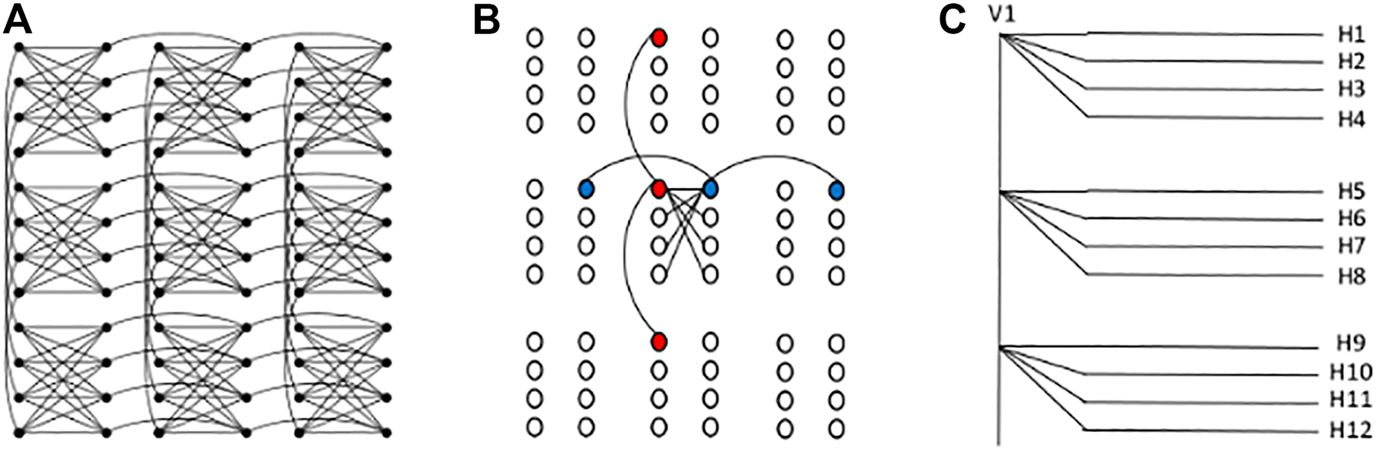
FIGURE 1. (A) C3 Chimera graph of qubits. (B) Three vertical (red) and horizontal (blue) qubits are chained to form a visible and a hidden unit. (C) Connectivity of a visible unit (V1) with 12 hidden units (H1 to H12). Here, each unit is formed by ferromagnetic couplings between three qubits.

2.4 Restricted Boltzmann Machine Embedding Onto the D-Wave QPU

Mapping an AQC algorithm on specific hardware is nontrivial and requires creative mapping. Several algorithms can be used to map a graph to the physical qubits on an adiabatic quantum computer [39, 40]. However, it is nontrivial to find a simple embedding when the graph size is large. Taking into consideration the arrangement of qubits on the 2000Q processor, we found a simple embedding that utilizes most of the working qubits. In the present study, we investigated RBMs in two configurations, one with 64 visible units and 64 hidden units, another with 64 visible units and 20 hidden units. Here, we will discuss the embedding of the RBM with 64 units in both layers. Each unit of the RBM is connected to 64 other units, but in the D-Wave each qubit only connects to six other qubits. To enhance the connectivity, qubits can be coupled together or cloned by setting $J_{i,j}=-1$. This forces the two qubits to stay in the same state. In our embedding, one unit of RBM is formed by connecting 16 qubits. The D-Wave processor has qubits arranged in $16\times 16$ matrices of unit cells. Each unit cell has two sets of four qubits arranged in a bipartite fashion. Each qubit in the left column of the unit cell can be connected to one qubit of the unit cell just above it and one just below it. There are 16 unit cells along one side, so a chain of 16 qubits can be formed. This chain forms one visible unit of the RBM. Figure 1B shows the procedure to couple three qubits to form a chain that represents a visible unit. The qubits that are connected together to form a vertical chain forming a visible unit are shown in red. Since there are four qubits in the left column of the unit cell, four chains can be formed resulting in four visible units of RBM. The four qubits that form the right column of the unit cell can be connected to form horizontal chains as shown in Figure 1B. These horizontal chains form the hidden units. There are 16 unit cells along the horizontal direction in a C16 Chimera graph, therefore each horizontal chain is also composed of 16 qubits. Utilizing the arrangement of qubits of the D-Wave QPU, 64 vertical and 64 horizontal chains can be formed representing the 64 visible and 64 hidden units of RBM. Figure 1C shows the scheme that we used to connect one visible unit (V1) to the hidden units. In this fashion, one can embed an RBM with 64 visible and 64 hidden units on a C16 Chimera graph. Of course, care must be taken for any inaccessible qubits to form a further restricted RBM. In our experiments, we found that the absence of a few qubits does not affect the performance of the resulting network.

2.5 Classification and Image Reconstruction

Each record of the bars and stripes dataset is made up of 64 bits. The last two bits are for labeling the pattern: 01 for a bar and 10 for a stripes pattern–Figure 2A. If the last two bits are 00 or 11, the prediction by RBM is incorrect. Once we obtained the weights and biases of the RBM from the training step, RBM can be used for classification or image reconstruction. To predict the class of a test record we apply its first 62 bits at the visible layer Figure 2B. We randomly input either zero or one for the last two classifying bits (L1 and L2). We then run 50 Gibbs cycles, keeping the 62 visible units clamped at the values of the test record. At the end of 50 Gibbs cycles label units, 63 and 64 are read. $L1=0$ and $L2=1$ indicates a bar pattern, while $L1=1$ and $L2=0$ suggests a stripe pattern. For the problem of image reconstruction, the goal is to predict the missing part of an image. A similar procedure can be applied for image reconstruction where a trained RBM is used to predict the values of the missing units. In this case, we clamp the visible units where values are given, and run 50 Gibbs cycles, at the end, we sample from the units where values have to be predicted.

FIGURE 2

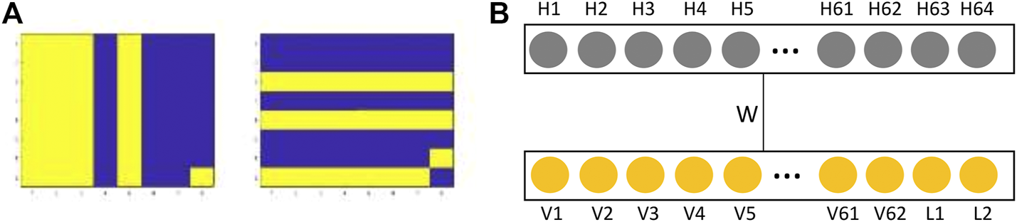
FIGURE 2. (A) Example of the bars (left) and stripes (right) patterns of size $8\times 8$. A blue cell represents a 0 while a yellow cell a 1. Last two bits (bottom right) are labels; bar = 01, stripe = 10. (B) RBM for classification. Box with yellow units is the visible layer. The hidden layer is shown by a box with grey units. $8\times 8$ bits of an image is rearranged into a record of size $1\times 64$ bits which is applied to the visible layer. Units L1 and L2 are the labels.

3 Results and Discussion

In the present work, we have used the bars and stripes (BAS) dataset. An example of a bar and a stripe pattern is shown in Figure 2A. BAS is a popular dataset for RBM training, it has been used by several researchers [22, 41–43]. This is a binary dataset consisting of records of 64 bits in length, with the last 2 bits representing the label of the record: 01 for a bar and 10 for a stripe pattern. Our dataset is comprised of 512 unique records. The number of unique samples used for training is 400, with the remaining 112 samples were held for testing. Classification of bars and stripes, image reconstruction, and the log-likelihood values are used to compare the performances of trained RBMs.

3.1 Restricted Boltzmann Machine Training

Equation 20 has been used to train the RBMs. The first term in this equation is a data-dependent term which can be exactly calculated using the conditional probabilities $P\left(h|v\right)$ and $P\left(v|h\right)$ given by Eq. 15 and Eq. 16. The second term is a model-dependent, which requires expectation value over all possible hidden h and visible v vectors, which is clearly intractable. Typically, the model-dependent term is approximately estimated using a method known as contrastive divergence (CD). In this approach, samples needed to calculate the model-dependent term are obtained by running the Gibbs chain starting from a sample from the training data (Figure 3). If n Gibbs steps are performed, the method is known as CD-n. It is shown by Hinton that $n=1$ could be sufficient for convergence (CD-1) [20]. In CD-1, first, a data sample is applied at the visible layer, then Eq. 15 is used to generate a corresponding hidden vector at the hidden layer. Now, this hidden vector is used to generate a new visible vector using Eq. 16, which is in turn used to generate a new hidden vector. These new visible and hidden vectors are used to calculate the model-dependent term. This process is repeated for each record in the dataset. A detailed description of RBM training using CD is given in a review article by Hinton [44]. The model-dependent term can also be calculated using samples (v and h) obtained from an RBM mapped on the D-Wave. From Eq. 19 we notice that in the second term the expectation value should be calculated with respect to $e^{-E\left(v,h\right)}$ distribution, while samples from the D-Wave follow a distribution of $e^{-\frac{E\left(v,h\right)}{kT}}$. It should be noted as the RBM training starts, the weights and biases are random, and samples from the D-Wave are not expected to have a Boltzmann distribution, however, as the training progresses the underlying probability distribution moves toward the Boltzmann distribution. Following the approach used by Adachi et al. [21], we used a hyperparameter, S, such that for the model-dependent term, we sample from $e^{\frac{-E\left(v,h\right)}{SkT}}$ distribution. Here, S is a hyperparameter, which is determined by the calculation of the classification accuracy for various values of S. The optimal condition corresponds to the case when $SkT=1$. A different approach was taken by Benedetti et al. [22]. They calculated effective temperature during each epoch. Their approach is difficult to apply in the present case of 64 bits record length BAS dataset. The BAS dataset that they used was comprised of just 16-bit records. A complex dataset leads to a complicated distribution, which makes training with a dynamical effective temperature difficult.

FIGURE 3

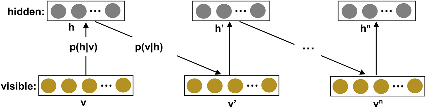
FIGURE 3. Illustration of the contrastive divergence algorithm for training a Restricted Boltzmann Machine (RBM). If sampling stops at $n_{th}$ Gibbs step of the Markov Chain, the procedure is known as CD-n.

In order to train an RBM using D-Wave, model parameters ($w_{ij}$, $b_i$ and $c_j$) were initialized with random values, the first term of Eq. 20 was calculated exactly using these weights and biases, and the training dataset. The weights and biases were then used to embed the RBM onto the D-Wave QPU, and quantum annealing was performed. Once annealing was complete, the D-Wave returned low energy solutions. Based on the mapping of the RBM, visible v and hidden h vectors were obtained from the solutions returned from the D-Wave. These v and h samples were used to calculate the model-dependent expectation value which in turn gives the gradient of log-likelihood. The gradient was further used to calculate new weights and biases (Eq. 24). The whole process was repeated until some convergence criterion was achieved. One of the several ways to monitor the progress of model learning during the RBM training is by estimating the reconstruction error for each training epochs. The reconstruction error is defined as:

$\text{Reconstruction}\text{error}={\displaystyle \sum }_{i=1}^n{\displaystyle \sum }_{t=1}^N{\left(v^{\left(t\right)}-v^{\prime }\right)}^2(26)$

where $v^{\left(t\right)}$ is a data record and $v\text{'}$ is the reconstructed visible vector (Figure 3). N and n are the number of records in the training dataset and the number of units in the visible layer, respectively. The plot of reconstruction error versus epoch is presented in the left panel of Figure 4. An optimal value of the empirical parameter S is important for a correct sampling of v and h vectors. The effect of change in S on the classification accuracy is shown in the right-side panel of Figure 4, a plot between accuracy and epoch. The term epoch means a full cycle of iterations, with each training pattern participating only once. Accuracy is defined as:

$\text{Accuracy}=\frac{\text{Number}\text{of}\text{correct}\text{predictions}}{\text{Total}\text{number}\text{of}\text{predictions}}(27)$

FIGURE 4

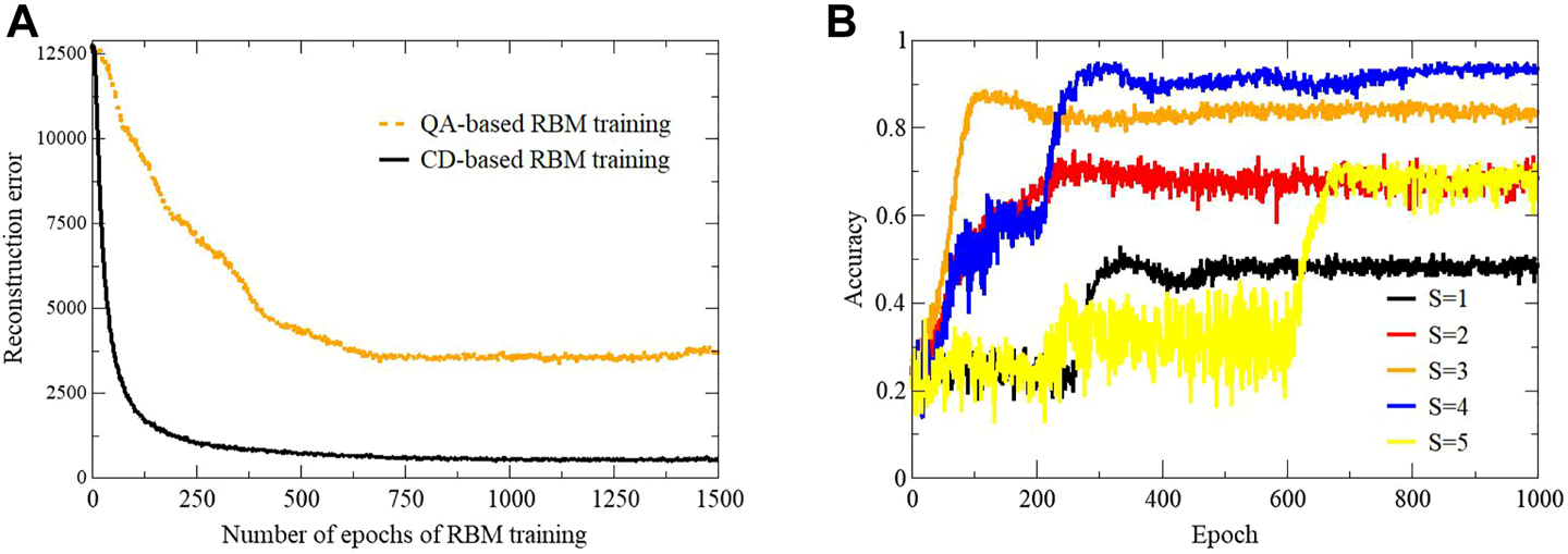
FIGURE 4. (A) Reconstruction error versus epoch of the RBM training. (B) The plot of the classification accuracy versus epoch for different values of the hyperparameter S.

The classification accuracy is maximum for $S=4$. The performance of the model during the training process can be visualized by plotting classification accuracy with epochs. Figure 5 shows the plot of classification accuracy vs. epochs for bars (left) and stripes (right) patterns. This calculation was performed on the test dataset. As the number of epoch increases from 0 to 400, the classification accuracy increases after that it stays constant. Based on these results, we conclude that the performance of QA-trained RBM is similar to CD-trained RBM. However, from Figure 5 we notice that there are higher fluctuations in the classification accuracy with CD-1 based training.

FIGURE 5

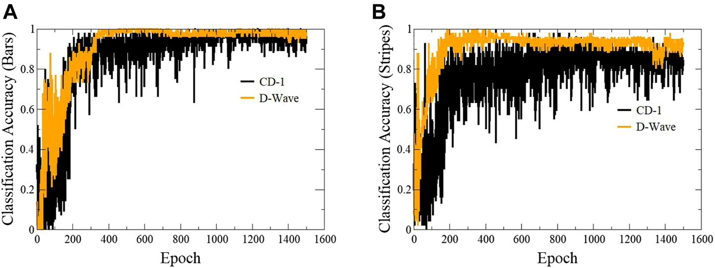
FIGURE 5. Plots showing classification accuracy of individual classes with epoch. The gradient of log-likelihood was calculated using samples generated via contrastive divergence and D-Wave’s quantum annealer. A comparison of classification accuracy for both methods is presented for bars (A) and stripes (B) patterns.

3.2 Image Reconstruction

For classification tasks, both training methods (QA and CD-1) showed similar results. Classification task requires the prediction of target labels (only 2 bits) based on the features in the dataset. An input data record is applied at the visible layer and the target labels are reconstructed. A more difficult task would be the reconstruction of not just the target labels, but also some other bits of the record. We call this task - image reconstruction. Here, we take a 64-bit record from the test dataset, corrupt some of its bits, and then apply this modified test record to the visible layer of a trained RBM. We follow the procedure explained earlier for the image reconstruction. The results of image reconstruction are presented in Figure 6. In Figure 6A, only target labels were corrupted/reconstructed. We notice that both training methods correctly reproduced the classifying labels. In the second case, Figure 6B, 16 bits of the original data record were corrupted. The RBM trained using CD-1 correctly predicted all the bit, while two bits were incorrectly predicted by the RBM trained with QA. In the third case, Figure 6C completely random 64-bit input vector (all bits corrupted) was fed to both RBMs. In the case of CD-1, the output is a bar pattern, whereas QA trained RBM resulted in a stripes pattern with many bits incorrectly predicted. Figure 6B shows a particular case where 16 bits of a record were corrupted and then reconstructed, histograms in the right panel of Figure 6 show the results when 16 bits of all the records of the dataset were corrupted and then reconstructed. These histograms show the plots between the number of instances of the dataset versus the number of incorrectly predicted bits. Figure 6D and Figure 6E show the results where CD-trained RBM was used for image reconstruction. Figure 6D shows the case where the records of the training data were corrupted and fed to a CD-trained RBM for performing the reconstruction. The histogram shows that in over 350 cases all the bits were correctly predicted. In the cases where some bits were not correctly predicted, the number of incorrectly predicted bits was less than or equal to eight. Figure 6E shows a similar histogram for the test dataset which had 112 records. Around 100 records were correctly predicted. Figure 6F and Figure 6G show the histogram for the cases where QA-based trained RBM was used for image reconstruction. In Figure 6F where records from the training dataset were used, for most of the instances around 4 bits were incorrectly predicted. Figure 6G shows the results for the case where the records from the test dataset were used for image reconstruction. In this case, most of the reconstructed images show about 6–7 bits incorrectly predicted. From these plots, it is clear that the CD-trained RBM performed better than the QA-trained RBMs.

FIGURE 6

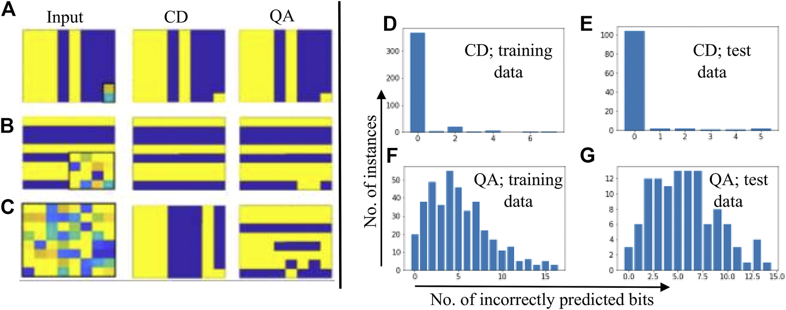
FIGURE 6. Original data was first corrupted, then reconstructed. Left panel: The images in the left column are input data fed to the RBMs; output obtained from the CD and QA-trained RBMs is shown in the middle and right column, respectively. The bits of the input images that were corrupted are enclosed in black boxes. Right panel: Histograms showing the distribution of incorrectly predicted bits versus the number of instances; 16 bits of the records were corrupted and then reconstructed using trained RBMs.

3.3 Log-likelihood Comparison

The classification accuracy results indicated similar performances of both methods (CD-1 and quantum annealing). However, image reconstruction suggests the improved performance of CD-1. In order to further compare and quantify the performances of these two methods, the log-likelihood of training data was calculated. Several researchers have used “log-likelihood” in order to compare different RBM models [45, 46]. The log-likelihood has been computed using Eq. 18. It involves the computation of the partition function Z. If the number of units in the hidden layer is not too large, Z can be exactly calculated using Eq. 7. To calculate the log-likelihood, the number of hidden units was set to 20. The log-likelihood of both models was computed at various epochs. The results are presented in Figure 7. From the figure, we notice that the log-likelihood is higher for RBM trained using CD-1 compared to quantum annealing. A lower value of the log-likelihood for the D-Wave trained model could be attributed to a restricted range of allowed values for the bias field h and the coupling coefficients J. Another reason could be an instance (each set of h and J) dependent temperature variation during the RBM training [22], which disturbs the learning of embedded RBM. Figure 7 also compares the log-likelihood values calculated using the new lower-noise D-Wave 2000Q processor and an earlier 2000Q processor. D-Wave’s lower-noise machine shows slightly improved log-likelihood values over the entire training range.

FIGURE 7

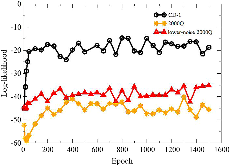
FIGURE 7. Plot showing variation in log-likelihood with training epochs. Label CD-1 represents CD-based RBM training, while label 2000Q indicates QA-based RBM training employing the D-Wave 2000Q.

3.4 Feature Reduction

Next, we compared the performance of a QA and CD-1 trained RBM for features reduction applications. Both RBMs that were used in this experiment had 64 visible and 20 hidden units. The BAS dataset was comprised of 62 binary features and two target labels. The target labels were removed and random 0 and 1s were added before feeding the dataset to an RBM for feature reduction. Input data vector from the training data was applied to the visible layer of the RBM. Equation 15 was then used to obtain the hidden variables. The compressed feature vector was sampled from 20 hidden units of the hidden layer. This procedure was used to extract features corresponding to 400 records of the training data and 112 records of the test data. Several classifiers were used to compare the effectiveness of feature reduction of QA and CD-1 trained RBMs. The results are presented in Table 1. Both feature reduction methods resulted in high classification accuracy, with classifiers trained on data obtained from CD-trained RBM showing slightly improved classification accuracy than the classifiers trained on data from a QA-trained RBM.

TABLE 1

TABLE 1. Comparison of classifiers trained on compressed BAS dataset obtained from CD-1 and QA trained RBMs. The classification accuracy was estimated on the test data comprised of 56 bars and 56 stripes instances. The label “No. of bars” (No. of stripes) indicates the number of correctly predicted bar (stripe) instances. The labels CD-1 and QA indicate that the feature reduction was performed using contrastive divergence and quantum annealing, respectively.

Currently, quantum computers are in their developmental stage. Therefore, the comparison of quantum annealing based RBM training with a mature classical approach like CD is uneven. However, such comparison is important as results from a CD trained RBM provides a reference with respect to which performance of QA based RBM training can be assessed. Though a better performance of CD was expected, QA performed satisfactorily. For classification and feature reduction tasks both QA and CD performed comparably. For the image reconstruction task, CD performed better than QA. The lower performance of QA-based training could be attributed to two main reasons. First, we obtain samples from the D-Wave assuming that it operates at a fixed temperature. However, this is an approximation, and one should calculate an effective temperature during each epoch. This mismatch degrades RBM’s learning during the training. Efforts have been made towards developing methods to estimate this instance-dependent temperature for small datasets [22, 23], none of which have been shown to be efficient for bigger datasets. Another reason for the lower performance of QA-trained RBM could be hardware limitations like limited connectivity, lower coherence time, noise, etc. These limitations will be removed as quantum annealing technology matures. D-Wave’s new machine, advantage, has higher connectivity, qubits and lower noise compared to the older machine. In Figure 7 we have shown that the new 2000Q machine performs better than the older machine. We believe as technology evolves and a new algorithm for calculation of effective temperature is developed QA based RBM training will improve and will be able to deal with larger datasets. Quantum annealing offers a fundamentally different approach to estimate model-dependent term of the gradient of log-likelihood compared to CD and PCD. Depending on the complexity of a dataset, the CD might need hundreds of Gibbs cycles to reach the equilibrium to finally give one sample, while using a QA-based approach one can obtain 10,000 samples almost instantaneously.

4 Conclusion

In this work, we present an embedding that can be used to embed an RBM with 64 visible and 64 hidden units. We trained an RBM by calculating the model-dependent term of the gradient of the log-likelihood using samples obtained from the D-Wave quantum annealer. The trained RBM was embedded onto the D-Wave QPU for classification and image reconstruction. We also showed that a new lower-noise quantum processor gives improved results. The performance of the RBM was compared with an RBM trained with a commonly used method called contrastive divergence (CD-1). Though both methods resulted in comparable classification accuracy, CD-1 training resulted in better image reconstruction and log-likelihood values. RBM training using the samples from a quantum annealer removes the need for time-consuming MCMC steps during training and classification procedures. These computationally expensive MCMC steps are an essential part of training and classification with CD-1. QA-based RBM learning could be improved by the calculation of an instance-dependent temperature and incorporating this temperature in the RBM training procedure though better methods to compute the effective temperature of the D-Wave machine on large datasets is still an open problem.

Data Availability Statement

The raw data supporting the conclusion of this article will be made available by the authors, without undue reservation.

Author Contributions

SK, TH, and MA designed the work, VD and RS performed the calculations. All authors discussed the results and wrote the paper.

Funding

We are grateful for the support from Integrated Data Science Initiative Grants (IDSI F.90000303), Purdue University. SK would like to acknowledges funding by the U.S. Department of Energy (Office of Basic Energy Sciences) under Award No. DE-SC0019215. TH would like to acknowledge funding by the U.S. Department of Energy (Office of Basic Energy Science) under Award No. ERKCG12. This manuscript has been authored by UT-Battelle, LLC under Contract No. DE-AC05-00OR22725 with the U.S. Department of Energy.

Conflict of Interest

The authors declare that the research was conducted in the absence of any commercial or financial relationships that could be construed as a potential conflict of interest.

Acknowledgments

The United States Government retains and the publisher, by accepting the article for publication, acknowledges that the United States Government retains a non-exclusive, paid-up, irrevocable, worldwide license to publish or reproduce the published form of this manuscript, or allow others to do so, for United States Government purposes. The Department of Energy will provide public access to these results of federally sponsored research in accordance with the DOE Public Access Plan. This manuscript has been released as a pre-print at arXiv:2005.03247 (cs.LG) [47].

References

1. Rieffel E, Polak W. Quantum Computing: A Gentle Introduction. Cambridge: MIT Press (2014).

2. Nielsen MA, Chuang IL. Quantum Computation and Quantum Information: 10th Anniversary Edition. Cambridge: Cambridge University Press (2010). doi:10.1017/CBO9780511976667

CrossRef Full Text

3. Kais S. Quantum Information and Computation for Chemistry. Hoboken, New Jersey: John Wiley & Sons (2014).

4. Farhi E, Goldstone J, Gutmann S, Sipser M. Quantum Computation by Adiabatic Evolution. arXiv preprint quant-ph/0001106 (2000).

Google Scholar

5. Aharonov D, van Dam W, Kempe J, Landau Z, Lloyd S, Regev O. Adiabatic Quantum Computation Is Equivalent to Standard Quantum Computation. SIAM J Comput (2007) 37:166–94. doi:10.1137/S0097539705447323

CrossRef Full Text | Google Scholar

6. Kadowaki T, Nishimori H. Quantum Annealing in the Transverse Ising Model. Phys Rev E (1998) 58:5355–63. doi:10.1103/PhysRevE.58.5355

CrossRef Full Text | Google Scholar

7. Finnila AB, Gomez MA, Sebenik C, Stenson C, Doll JD. Quantum Annealing: A New Method for Minimizing Multidimensional Functions. Chem Phys Lett (1994) 219:343–8. doi:10.1016/0009-2614(94)00117-0

CrossRef Full Text | Google Scholar

8. Santoro GE, Tosatti E. Optimization Using Quantum Mechanics: Quantum Annealing through Adiabatic Evolution. J Phys A: Math Gen (2006) 39:R393–R431. doi:10.1088/0305-4470/39/36/r01

CrossRef Full Text | Google Scholar

9. Das A, Chakrabarti BK. Colloquium: Quantum Annealing and Analog Quantum Computation. Rev Mod Phys (2008) 80:1061–81. doi:10.1103/RevModPhys.80.1061

CrossRef Full Text | Google Scholar

10. Albash T, Lidar DA. Adiabatic Quantum Computation. Rev Mod Phys (2018) 90:015002. doi:10.1103/RevModPhys.90.015002

CrossRef Full Text | Google Scholar

11. Boixo S, Rønnow TF, Isakov SV, Wang Z, Wecker D, Lidar DA, et al. Evidence for Quantum Annealing with More Than One Hundred Qubits. Nat Phys (2014) 10:218–24. doi:10.1038/nphys2900

CrossRef Full Text | Google Scholar

12. Biamonte JD, Love PJ. Realizable Hamiltonians for Universal Adiabatic Quantum Computers. Phys Rev A (2008) 78:012352. doi:10.1103/physreva.78.012352

CrossRef Full Text | Google Scholar

13. Mott A, Job J, Vlimant J-R, Lidar D, Spiropulu M. Solving a Higgs Optimization Problem with Quantum Annealing for Machine Learning. Nature (2017) 550:375–9. doi:10.1038/nature24047

PubMed Abstract | CrossRef Full Text | Google Scholar

14. Das S, Wildridge AJ, Vaidya SB, Jung A. Track Clustering with a Quantum Annealer for Primary Vertex Reconstruction at Hadron Colliders. arXiv preprint arXiv:1903.08879 (2019).

Google Scholar

15. Ushijima-Mwesigwa H, Negre CFA, Mniszewski SM. Graph Partitioning Using Quantum Annealing on the D-Wave System. In: Proceedings of the Second International Workshop on Post Moores Era Supercomputing, PMES’17. Denver, CO: ACM (2017). p. 22–9.

Google Scholar

16. O'Malley D, Vesselinov VV, Alexandrov BS, Alexandrov LB. Nonnegative/binary Matrix Factorization with a D-Wave Quantum Annealer. PLOS ONE (2018) 13:1–12. doi:10.1371/journal.pone.0206653

CrossRef Full Text | Google Scholar

17. Li RY, Di Felice R, Rohs R, Lidar DA. Quantum Annealing versus Classical Machine Learning Applied to a Simplified Computational Biology Problem. Npj Quan Inf (2018) 4:14. doi:10.1038/s41534-018-0060-8

CrossRef Full Text | Google Scholar

18. Jiang S, Britt KA, McCaskey AJ, Humble TS, Kais S. Quantum Annealing for Prime Factorization. Sci Rep (2018) 8:17667. doi:10.1038/s41598-018-36058-z

PubMed Abstract | CrossRef Full Text | Google Scholar

19. Xia R, Bian T, Kais S. Electronic Structure Calculations and the Ising Hamiltonian. J Phys Chem B (2018) 122:3384–95. doi:10.1021/acs.jpcb.7b10371

PubMed Abstract | CrossRef Full Text | Google Scholar

20. Hinton GE. Training Products of Experts by Minimizing Contrastive Divergence. Neural Comput (2002) 14:1771–800. doi:10.1162/089976602760128018

PubMed Abstract | CrossRef Full Text | Google Scholar

21. Adachi SH, Henderson MP. Application of Quantum Annealing to Training of Deep Neural Networks. arXiv preprint arXiv:1510.06356 (2015).

Google Scholar

22. Benedetti M, Realpe-Gómez J, Biswas R, Perdomo-Ortiz A. Estimation of Effective Temperatures in Quantum Annealers for Sampling Applications: A Case Study with Possible Applications in Deep Learning. Phys Rev A (2016) 94:022308. doi:10.1103/PhysRevA.94.022308

CrossRef Full Text | Google Scholar

23. Caldeira J, Job J, Adachi SH, Nord B, Perdue GN. Restricted Boltzmann Machines for Galaxy Morphology Classification with a Quantum Annealer. arXiv preprint arXiv:1911.06259 (2019).

Google Scholar

24. Sleeman J, Dorband J, Halem M. A Hybrid Quantum Enabled Rbm Advantage: Convolutional Autoencoders for Quantum Image Compression and Generative Learning (2020), April 27–May 9, 2020, California: Society of Photo-Optical Instrumentation Engineers (SPIE).

25. Winci W, Buffoni L, Sadeghi H, Khoshaman A, Andriyash E, Amin MH. A Path towards Quantum Advantage in Training Deep Generative Models with Quantum Annealers. Mach Learn Sci Technol (2020) 1:045028. doi:10.1088/2632-2153/aba220

CrossRef Full Text | Google Scholar

26. Korenkevych D, Xue Y, Bian Z, Chudak F, Macready WG, Rolfe J. Benchmarking Quantum Hardware for Training of Fully Visible Boltzmann Machines (2016).

27. Rocutto L, Destri C, Prati E. Quantum Semantic Learning by Reverse Annealing of an Adiabatic Quantum Computer. Adv Quan Tech (2021) 4:2000133. doi:10.1002/qute.202000133

CrossRef Full Text | Google Scholar

28. Koshka Y, Novotny MA. Comparison of D-Wave Quantum Annealing and Classical Simulated Annealing for Local Minima Determination. IEEE J Sel Areas Inf Theor (2020) 1:515–25. doi:10.1109/JSAIT.2020.3014192

CrossRef Full Text | Google Scholar

29. Dumoulin V, IanGoodfellow JAC, Bengio Y. On the Challenges of Physical Implementations of Rbms. In: AAAI Publications, Twenty-Eighth AAAI Conference on Artificial Intelligence (2014) Quebec, Canada, July 27–31, 2014.

Google Scholar

30. Koshka Y, Novotny MA. Comparison of Use of a 2000 Qubit D-Wave Quantum Annealer and Mcmc for Sampling, Image Reconstruction, and Classification. IEEE Trans Emerg Top Comput Intell (2021) 5:119–29. doi:10.1109/TETCI.2018.2871466

CrossRef Full Text | Google Scholar

31. Koshka Y, Novotny MA. 2000 Qubit D-Wave Quantum Computer Replacing Mcmc for Rbm Image Reconstruction and Classification. In: 2018 International Joint Conference on Neural Networks (IJCNN); July 8–13, 2018, Rio de Janeiro, Brazil (2018). p. 1–8. doi:10.1109/IJCNN.2018.8489746

CrossRef Full Text | Google Scholar

32. Koshka Y, Perera D, Hall S, Novotny MA. Determination of the Lowest-Energy States for the Model Distribution of Trained Restricted Boltzmann Machines Using a 1000 Qubit D-Wave 2x Quantum Computer. Neural Comput (2017) 29:1815–37. doi:10.1162/neco_a_00974

PubMed Abstract | CrossRef Full Text | Google Scholar

33. Koshka Y, Perera D, Hall S, Novotny MA. Empirical Investigation of the Low Temperature Energy Function of the Restricted Boltzmann Machine Using a 1000 Qubit D-Wave 2X. In: 2016 International Joint Conference on Neural Networks (IJCNN); July 24–29, 2016, Vancouver, BC(2016). p. 1948–54. doi:10.1109/IJCNN.2016.7727438

CrossRef Full Text | Google Scholar

34. Dixit V, Selvarajan R, Aldwairi T, Koshka Y, Novotny MA, Humble TS. Training a Quantum Annealing Based Restricted Boltzmann Machine on Cybersecurity Data. In: IEEE Transactions on Emerging Topics in Computational Intelligence (2021).

Google Scholar

35. Amin MH, Andriyash E, Rolfe J, Kulchytskyy B, Melko R. Quantum Boltzmann Machine. Phys Rev X (2018) 8:021050. doi:10.1103/PhysRevX.8.021050

CrossRef Full Text | Google Scholar

36. Lloyd S, Mohseni M, Rebentrost P. Quantum Algorithms for Supervised and Unsupervised Machine Learning. arXiv preprint arXiv:1307.0411 (2013).

Google Scholar

37. Rebentrost P, Mohseni M, Lloyd S. Quantum Support Vector Machine for Big Data Classification. Phys Rev Lett (2014) 113:130503. doi:10.1103/PhysRevLett.113.130503

PubMed Abstract | CrossRef Full Text | Google Scholar

38. Wiebe N, Kapoor A, Svore KM. Quantum Deep Learning. arXiv preprint arXiv:1412.3489 (2014).

Google Scholar

39. Goodrich TD, Sullivan BD, Humble TS. Optimizing Adiabatic Quantum Program Compilation Using a Graph-Theoretic Framework. Quan Inf Process (2018) 17:1–26. doi:10.1007/s11128-018-1863-4

CrossRef Full Text | Google Scholar

40. Date P, Patton R, Schuman C, Potok T. Efficiently Embedding Qubo Problems on Adiabatic Quantum Computers. Quan Inf Process (2019) 18:117. doi:10.1007/s11128-019-2236-3

CrossRef Full Text | Google Scholar

41. Krause O, Fischer A, Igel C. Population-contrastive-divergence: Does Consistency Help with Rbm Training?. Pattern Recognition Lett (2018) 102:1–7. doi:10.1016/j.patrec.2017.11.022

CrossRef Full Text | Google Scholar

42. Schulz H, Müller A, Behnke S. Investigating Convergence of Restricted Boltzmann Machine Learning. In: NIPS 2010 Workshop on Deep Learning and Unsupervised Feature Learning; December 2010, Whistler, Canada, 1 (2010). p. 6–1.

Google Scholar

43. Upadhya V, Sastry P. Learning Rbm with a Dc Programming Approach. arXiv preprint arXiv:1709.07149 (2017).

Google Scholar

44. Hinton GE. A Practical Guide to Training Restricted Boltzmann Machines. Berlin, Heidelberg: Springer (2012). p. 599–619. doi:10.1007/978-3-642-35289-8_32

CrossRef Full Text

45. Tieleman T. Training Restricted Boltzmann Machines Using Approximations to the Likelihood Gradient. In: Proceedings of the 25th International Conference on Machine Learning, ICML ’08. New York, NY, USA: ACM (2008). p. 1064–71. doi:10.1145/1390156.1390290

CrossRef Full Text | Google Scholar

46. Cho K, Raiko T, Ilin A. Parallel Tempering Is Efficient for Learning Restricted Boltzmann Machines. In: The 2010 International Joint Conference on Neural Networks (IJCNN); July 18–23, 2010, Barcelona, Spain (2010). p. 1–8. doi:10.1109/IJCNN.2010.5596837

CrossRef Full Text | Google Scholar

47. Dixit V, Selvarajan R, Alam MA, Humble TS, Kais S. Training and Classification Using a Restricted Boltzmann Machine on the D-Wave 2000Q. arXiv preprint arXiv:2005.03247 (2020).

Google Scholar