Role of Homoclinic Breathers in the Interpretation of Experimental Measurements, With Emphasis on the Peregrine Breather

Introduction

The nonlinear Schrödinger equation in one-space and one-time dimensions (1+1) has been a useful, but simple model for the study of nonlinear waves in many fields of study, including physical oceanography, ocean engineering and nonlinear optics [1–6]. The general periodic/quasiperiodic solutions of NLS equation consist of ratios of Riemann theta functions that have differing phases [7–9]. The general Riemann (nonlinear) spectrum is described parametrically by the Riemann matrix. The diagonal elements of the Riemann matrix are the Stokes wave solutions of NLS and the off-diagonal elements describe the interactions among Stokes waves. When spectral components have a Benjamin-Feir parameter greater than one, then two Stokes modes will phase lock with one another, thereby creating a breather, i.e., a wave packet that “breathes” up and down during its evolution. The maximum amplitude of a breather during its nonlinear motion has a central enhanced carrier wave that is often referred to as a “rogue” or “freak” wave. The work of Peregrine identified one particular breather of exceptional simplicity: The ratio of two low degree polynomials. Peregrine called such solutions “sudden steep events” although the field of nonlinear waves has chosen the term “breathers” instead, due to the naming convention used in early theoretical work (see for example [10]). The field has grown tremendously in the past 30 years because it has captured the imagination of a large number of investigators interested in freak wave behavior in ocean waves and in nonlinear optics.

There are a large number of “coherent structures” in the nonlinear Schrödinger equation. For example in shallow water there are Stokes waves, dark solitons and “ghost” or “fossil” wave packets. In deep water there are also Stokes waves, bright solitons and breathers. Deep-water breathers are essentially phase-locked Stokes waves or solitons. The general solutions of the Schrödinger equation are determined from the ratio of multidimensional Riemann theta functions and these solutions contain all of the special cases of coherent structures just mentioned. Furthermore, it is known that the multidimensional theta function solutions can be reduced to the so-called N-soliton limit of NLS equation. How then does the Peregrine breather fit into all of this mathematical physics? The answer is that the above multidimensional solutions can be reduced to the so-called general homoclinic solutions, which occur in the soliton limit, by introducing periodic/quasiperiodic boundary conditions. The general homoclinic solutions can then be reduced to the Akhmediev, Peregrine and Kuznetzov-Ma breathers as special cases. Of course there is a continuous range of homoclinic solutions that provide a broad spectrum of breathers. Experimentally, if one is studying a quasiperiodic, multidimensional simulation or space/time series measurement of ocean waves, then it is not easy to pick out by eye from a seemingly random wave train what the actual coherent modes are. This has lead to a guessing game of trying to decide what particular modes are present in a selected time series measurement. This conundrum has led to the implementation of nonlinear Fourier methods for analyzing data [5], [11–13]. While details of this latter topic are treated elsewhere, the main goal of the present paper is to discuss the role that coherent structures play in solutions of the NLS equation and in the analysis of data. In this way one is able to identify their particular spectral signature in the nonlinear Fourier scheme, thus enabling experimentalists to better understand the physics of coherent structures in measured ocean waves.

The goal of this paper is to investigate a large general class of rogue wave breather solutions previously studied by [14, 15] and how they can be derived from Riemann theta functions. Herein I describe a simple breather solution that parametrically depends on a single eigenvalue that lies on the imaginary axis of the Riemann spectrum or so-called lambda plane (the Riemann surface) of the 1+1 NLS equation. Three particular eigenvalues give the most well known breathers used in the field today and due to [16, 17]; and [14, 18].

The results given herein have implications on the modern theoretical and experimental study of coherent structures and breather trains in both one and two dimensions. Recent exciting studies of nonlinear waves and their coherent properties for the ocean and laboratory have been made by a number of authors, including [5], [11], [19–26]. A central goal of this paper is to show how to use generalized homoclinic solutions to analyze space/time series data together with the Zakharov-Shabat eigenvalue problem, as described by Osborne and co-workers [5], [11], [12].

Integrability and Coherent Structures for 1D Water Waves

We consider water wave solutions of the nonlinear Schrödinger (NLS) equation

$i{u}_t+u_{xx}+2\sigma {\left|u\right|}^{2}u=0(1)$

The parameter $\sigma$ sigma can be $\pm 1$. The plus sign ($\sigma =+1$) occurs for deep-water waves such that $kh>1.363$ where the modulational instability exists and the Benjamin-Feir instability governs the nonlinear wave dynamics. In shallow water ($\sigma =-1$, where $kh<1.363$) the wave solutions are always stable. Detailed discussions of the NLS equation in terms of the theory of the inverse scattering method are given elsewhere [27], [9] (applications to ocean waves are given in [5]).

NLS equation has well-known coherent structures including Stokes waves, bright solitons, dark solitons and breathers. From the point of view of the mathematical physics a single Stokes wave or soliton is a genus-1 solution of the nonlinear Schrödinger equation. Cases for bright and dark solitons are shown in Figure 1. The bright soliton solutions are associated with infinite line boundary conditions, while the dark solution solutions are related to a finite condition at infinity (or periodic boundary conditions). Thus Stokes waves are single-degree of freedom solutions and for the increasing nonlinear limit they morph these into soliton solutions (for the periodicity requirement often used in the study of water waves means that soliton trains are a feature of the method). Breathers are formed from the phase locking of two Stokes waves in the genus-2 case, an example of which is shown in Figure 2.

FIGURE 1

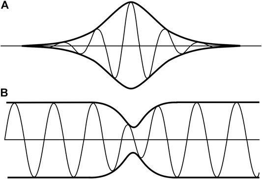
FIGURE 1. (A) A deep water envelope or bright soliton of the NLS equation (the thin line is the surface wave elevation and the thick line is the modulus of the envelope of NLS equation) and (B) a shallow water dark soliton (where the thin line is the surface elevation and the thick line is the modulus of the envelope of NLS equation).

FIGURE 2

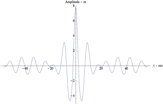
FIGURE 2. Breather solution of the nonlinear Schrödinger equation at the moment when it reaches maximum amplitude.

Of course a great deal of effort has been made to determine if the methods of soliton physics can be useful in the study of coherent structures in ocean waves. This is an important issue because the usual paradigm for nonlinear ocean waves is that for the 4-wave interactions where ocean waves are assumed to be weakly interacting sine waves. Thus a new approach, which is able to determine the behavior of nonlinear ocean waves from the point of view of their coherent structures, is a significant step beyond current understanding of quasilinear methods. Of course one has to extend the approach beyond one dimension to the two-dimensional equations such as NLS and its subsequent orders of approximation [28–31] equations. We are focused here on the 1D case where we attempt to bring together the complete set of ideas with regard to both infinite-line boundary conditions and periodic boundary conditions for the NLS equation. We are interested in the Stokes waves, soliton and breather solutions of the equation. Thus considerations with regard to infinite-line inverse scattering theory and the periodic solutions of inverse scattering theory are addressed. Why study IST? Because it provides one approach to study methods that allow one to nonlinearly Fourier analyze data to understand the role of coherent structures in ocean wave data [5], [11], [12].

Special and General Solutions of the NLS Equation

We discuss the special solution of the NLS equation, which are known to have homoclinic solutions. These include soliton solutions for both the shallow and deep-water NLS equations and for the deep-water theta function solutions.

Dark Soliton Solutions in Shallow Water

Given the nonlinear Schrödinger equation in shallow water, with complex solution $u(x,t)$

$i{u}_t+u_{xx}-2{\left|u\right|}^{2}u=0(2)$

[32] first wrote down the Dark soliton solutions of Eq. 2. This is written as the ratio of two functions:

$u\left(x,t\right)=a\frac{g\left(x,t\right)}{f\left(x,t\right)}{e}^{-2i{a}^{2}t}(3)$

where

$\begin{array}{l}f={\displaystyle \sum _{{\mu }_1=0}^1{\displaystyle \sum _{{\mu }_2=0}^1{e}^{{\displaystyle \sum _{j>k}^N{\mu }_i{\mu }_j{A}_{ij}}+{\displaystyle \sum _{i=1}^N{\mu }_i\left(k_{i}x-{\Omega }_{i}t+{\gamma }_i\right)}}}}\\ g={\displaystyle \sum _{{\mu }_1=0}^1{\displaystyle \sum _{{\mu }_2=0}^1{e}^{{\displaystyle \sum _{j>k}^N{\mu }_i{\mu }_j{A}_{ij}}+{\displaystyle \sum _{i=1}^N{\mu }_i\left(k_{i}x-{\Omega }_{i}t+{\gamma }_i+2i{\varphi }_i\right)}}}}\end{array}(4)$

where

$A_{ij}=\ln {\left[\frac{\sin \left(\frac{1}{2}\left({\varphi }_j-{\varphi }_k\right)\right)}{\sin \left(\frac{1}{2}\left({\varphi }_j+{\varphi }_k\right)\right)}\right]}^2$

$k_j=2a\sin {\varphi }_j$

${\Omega }_j=\pm k_j{\left(4a^2-k_j^2\right)}^{1/2}$

Here ${\gamma }_j$ are arbitrary constants.

A dark, or more correctly a gray, soliton is shown in Figure 1B. These are the single soliton solutions modes of the above multisoliton solution, which individually have the form:

${\left|u\left(x,t\right)\right|}^2={\rho }^2-\frac{k^2/4}{{\cosh }^2\left[\frac{1}{2}\left(kx-\Omega t\right)\right]}$

Bright Soliton Solutions in Deep Water

The nonlinear Schrödinger equation for deep water, with complex solution $\psi (x,t)$

$i{u}_t+u_{xx}+2{\left|u\right|}^{2}u=0(5)$

[33] derived the bright N-soliton packet solutions of Eq. 5. We seek a solution as the ratio of two functions:

$u(x,t)=\frac{G(x,t)}{F(x,t)}(6)$

At this stage we can “separate the variables” and set

$\begin{array}{l}i\left(G_{t}F-G{F}_t\right)+\mu \left(G_{xx}F-2G_x{F}_x+G{F}_{xx}\right)=0\\ 2\left(F{F}_{xx}-F_x^2\right)-{\left|G\right|}^2=0\end{array}(7)$

From the second of Eq. 7 get

${\left|\psi \right|}^2=\frac{G{G}^{\ast }}{F^2}=2{\partial }_{xx}\ln F(8)$

At this point the N-soliton solution arises as before by suitable exponential expansions:

$F={\displaystyle \sum _{{\mu }_1=0}^1{\displaystyle \sum _{{\mu }_2=0}^1\mathrm{...}{\displaystyle \sum _{{\mu }_N=0}^1{D}_1\left({\mu }_1,{\mu }_2\right)e^{{\displaystyle \sum _{1\le i<j}{\mu }_i{\mu }_j{A}_{ij}+{\displaystyle \sum _{i=1}^{2N}{\mu }_i\left(k_{i}x-{\Omega }_{i}t+{\varphi }_i\right)}}}}}}(9)$

$G={\displaystyle \sum _{{\mu }_1=0}^1{\displaystyle \sum _{{\mu }_2=0}^1\mathrm{...}{\displaystyle \sum _{{\mu }_N=0}^1{D}_2\left({\mu }_1,{\mu }_2\right)e^{{\displaystyle \sum _{1\le i<j}{\mu }_i{\mu }_j{A}_{ij}+{\displaystyle \sum _{i=1}^{2N}{\mu }_i\left(k_{i}x-{\Omega }_{i}t+{\varphi }_i\right)}}}}}}$

where

$k_{i+N}=k_i^{\ast }{\Omega }_{i+N}={\Omega }_i^{\ast }{\varphi }_{i+N}={\varphi }_i^{\ast };{\Omega }_i=-i{k}_i^{2}i=\mathrm{1,2...}N$

$A_{ij}=\ln \left[\frac{1}{2}{\left(k_i+k_j\right)}^{-2}\right]\mathrm{for}=\mathrm{1,2}\dots N\mathrm{and}j=N+1,N+2\dots 2N$

$A_{ij}=\ln \left[\frac{1}{2}{\left(k_i-k_j\right)}^{-2}\right]\mathrm{for}=N+1,N+\mathrm{2...2}N\mathrm{and}j=N+1,N+\mathrm{2...2}N$

and

$D_1\left({\mu }_1,{\mu }_2\right)=\{\begin{array}{cc}1& \mathrm{when}{\displaystyle \sum _{i=1}^N{\mu }_i={\displaystyle \sum _{i=1}^N{\mu }_{i+N}}}\\ 0& \mathrm{otherwise}\end{array}$

$D_2({\mu }_1,{\mu }_2)=\{\begin{array}{cc}1& \mathrm{when}1+{\displaystyle \sum _{i=1}^N{\mu }_{i+N}}={\displaystyle \sum _{i=1}^N{\mu }_i}\\ 0& \mathrm{otherwise}\end{array}$

This formulation gives the multisoliton solutions of the NLS equation for bright solitons on the infinite line.

A single bright soliton packet solution that has the form:

$u(x,t)=a\mathrm{sech}\left[a{\left|\frac{\nu }{2\mu }\right|}^{1/2}(x-Vt)\right]e^{i\left(\frac{V}{2\mu }x-\frac{V^2}{4\mu }t+\frac{1}{2}\nu a^{2}t\right)}$

Here V is an arbitrary group speed and a is an arbitrary amplitude. This solution can be seen in Figure 1A above.

Stokes Wave Solutions With Riemann Theta Functions for Periodic Boundary Conditions

The Riemann theta function solution of the NLS equation for deep water Eq. 5 is given by [9], [5]:

$u\left(x,t\right)=A\frac{\theta \left(x,t|\mathbf{\tau },{\delta }^{-}\right)}{\theta \left(x,t|\mathbf{\tau },{\delta }^{+}\right)}{e}^{2i{A}^{2}t}(10)$

The $\theta \left(x,t|\mathbf{\tau },\delta \right)$ are generalized Fourier series known as N-dimensional Riemann theta functions:

$\begin{array}{l}\theta \left(x,t|\tau ,{\delta }^{\pm }\right)=\\ ={\displaystyle \sum _{m_1=-\infty }^{\infty }{\displaystyle \sum _{m_2=-\infty }^{\infty }\dots {\displaystyle \sum _{m_N=-\infty }^{\infty }\exp i\left[{\displaystyle \sum _{n=1}^N{m}_n{K}_{n}x}+{\displaystyle \sum _{n=1}^N{m}_n{\Omega }_{n}t}+{\displaystyle \sum _{n=1}^N{m}_n{\delta }_n^{\pm }}+{\displaystyle \sum _{j=1}^N{\displaystyle \sum _{k=1}^N{m}_j{m}_k{\tau }_{jk}}}\right]}}}\end{array}(11)$

where the $K_n$ are wavenumbers, the ${\Omega }_n$ are frequencies, the ${\delta }_n^{\pm }$ are phases and ${\tau }_{mn}$ is the Riemann matrix, in which the diagonal elements correspond to Stokes waves and the off-diagonal elements refer to nonlinear interactions amongst the Stokes waves.

An important case is for the 2 × 2 period matrix, τ, which implies that $N=2$, a case considered in detail by [8]. For $N=2$ the theta function has the form:

$\theta (x,t|\mathit{\tau },{\mathit{\delta }}^{\pm })={\displaystyle \sum _{m_1=-\infty }^{\infty }{\displaystyle \sum _{m_2=-\infty }^{\infty }\exp i \left[{\displaystyle \sum _{n=1}^2{m}_n{K}_{n}x+{\displaystyle \sum _{n=1}^2{m}_n{\Omega }_{n}t+{\displaystyle \sum _{n=1}^2{m}_n{\delta }_n^{\pm }+{\displaystyle \sum _{j=1}^2{\displaystyle \sum _{k=1}^2{m}_j{m}_k{\tau }_{jk}}}}}}\right]}}(12)$

The parameters in the theta function are given by [5]:

• Expansion Parameters and Riemann Sheet Indices

${\epsilon }_1={\epsilon }_o{e}^{i\theta }{\epsilon }_2={\epsilon }_1^{\ast }$

${\sigma }_1=1{\sigma }_2=-1(13)$

• Spectral Eigenvalue

${\lambda }_1={\lambda }_R+i{\lambda }_I{\lambda }_2={\lambda }_1^{\ast }(14)$

• Spectral Wavenumber

$K_1=-2\sqrt{A^2+{\lambda }_1^2}{K}_2=-2\sqrt{A^2+{\lambda }_2^2}(15)$

• Spectral Frequency

${\Omega }_1=2{\lambda }_1{K}_1{\Omega }_2=2{\lambda }_2{K}_2(16)$

• Period Matrix

${\tau }_{11}=\frac{1}{2}+\frac{i}{\pi }\ln \left(\frac{K_1^2}{{\epsilon }_1}\right){\tau }_{12}=\frac{i}{2\pi }\ln \left(\frac{1+{\lambda }_1{\lambda }_2+\frac{1}{4}{K}_1{K}_2}{1+{\lambda }_1{\lambda }_2-\frac{1}{4}{K}_1{K}_2}\right)(17)$

${\tau }_{21}={\tau }_{12}{\tau }_{22}=\frac{1}{2}+\frac{i}{\pi }\ln \left(\frac{K_2^2}{{\epsilon }_2}\right)(18)$

• Phases

${\delta }_1^{+}=\pi +i\ln \left({\lambda }_1-\frac{1}{2}{K}_1\right)+i\ln \left({\sigma }_1{\lambda }_1+\frac{1}{2}{K}_1\right)$

${\delta }_1^{-}=\pi +i\ln \left({\lambda }_1+\frac{1}{2}{K}_1\right)+i\ln \left({\sigma }_1{\lambda }_1+\frac{1}{2}{K}_1\right)$

${\delta }_2^{+}=\pi +i\ln \left({\lambda }_2-\frac{1}{2}{K}_2\right)+i\ln \left({\sigma }_2{\lambda }_2-\frac{1}{2}{K}_2\right)$

${\delta }_2^{-}=\pi +i\ln \left({\lambda }_2+\frac{1}{2}{K}_2\right)+i\ln \left({\sigma }_2{\lambda }_2-\frac{1}{2}{K}_2\right)(19)$

Use of the above formulas in the theta function provides a simple way to compute the breather trains for the particular case of a modulated plane wave carrier.

Homoclinic Solutions

There are several ways the general homoclinic solutions can be derived. These are listed below:

1) The general methods of [14, 17, 18] and [16]. These are the classical approaches, are well known and will not be discussed further here.

2) From dark 2-soliton solutions (2)–(4). This has been discussed by [34] in considerable detail (see also [15]). The method begins with the dark N-soliton solutions as discuss above (3), (4). This approach provides an important connection between the dark solitons and homoclinic solutions.

3) From Stokes wave solutions with Riemann Theta Functions for periodic boundary conditions. These solutions can be used to determine the homoclinic solutions by letting the parameter $\epsilon \to 0$, as given by [35]. Likewise we can take the theta function solutions in the soliton limit to determine the deep-water N-soliton solution (5)–(9).

4) From bright 2-soliton solutions (5)–(9), by invoking periodic boundary conditions for the deep-water NLS Eq. 5 we can directly compute the homoclinic solution.

All of the above methods provide keen insight into the generalized homoclinic solutions (see Generalized Homoclinic Solution below) and their relationship to the inverse scattering transform. Why however do we care about homoclinic solutions from a physical standpoint?

• (a) For large oceanic wave fields the breathers tend to have spectral components clustered about the peak of the spectrum, and hence are homoclinic. Homoclinicity is a found in Mother Nature for extreme sea states and the homoclinic solutions are good physical approximations for the Fourier components in time series data.

• (b) Homoclinic solutions are simple, i.e., they are written in terms of trigonometric functions, not in terms of theta functions.

• (c) The simple homoclinic formulas are the “nonlinear Fourier modes” that are associated with each of the largest modes in the nonlinear spectrum. Since these modes have parameters that can be determined from time series by solving the Zakharov-Shabat eigenvalue problem for periodic boundary conditions [5], we know that the homoclinic modes uniquely describe each breather train in the measured time series. Therefore one might think of locating each measured breather train and comparing it with the homoclinic solution for the appropriate nonlinear Fourier component.

Let us now look at the generalized homoclinic solution of 1+1 NLS and discuss some of its properties.

Generalized Homoclinic Solution

The nonlinear Schrödinger equation in deep water is given by Eq. 5. Herein, we are interested in spatially periodic boundary conditions $\left(u\left(x,t\right)=u\left(x+L,t\right)\right)$ for which a large class of homoclinic solutions whose derivations are discussed above in Integrability and Coherent Structures for 1D Water Waves, and which are given by [14, 15, 34]:

$u\left(x,t\right)=a\left(\frac{1-2\cos \left(Kx\right)e^{\Omega t-2i\varphi +\gamma }+A{e}^{2\Omega t-4i\varphi +2\gamma }}{1-2\cos \left(Kx\right)e^{\Omega t+\gamma }+A{e}^{2\Omega t+2\gamma }}\right)e^{2i{a}^{2}t}(20)$

where

$\Omega =K\sqrt{4a^2-K^2}\left(\mathrm{Frequency}\right)(21)$

$K=2a\sin \varphi \left(\mathrm{Wavenumber}\right)(22)$

$L=\frac{2\pi }{K}=\frac{\pi }{a\sin \varphi }\left(\mathrm{Wavelength}\right)(23)$

$A={\sec }^2\varphi =\frac{1}{{\cos }^2\varphi }(24)$

Here a is the amplitude of the carrier wave. Notice that the parameter $\gamma$ may be interpreted as just a temporal phase shift and could just as well be omitted. However, I use $\gamma$ to keep the maximum of the waveform at the origin, $u_{\max }=u\left(\mathrm{0,0}\right)$. The presence of the parameter ϕ is the only difference between the numerator and denominator and is fundamental for describing modulational solutions of the NLS equation.

Some observations are in order here with respect to relating the above solution to the inverse scattering transform (IST) that I discuss further in Comments on Data Analysis. Clearly $\varphi$ must be related to the periodic IST eigenvalue¹ in the so-called $\lambda$-plane, where the Floquet problem for the Zakharov-Shabat eigenvalue problem is solved. Recall that the wavenumber is related to $\lambda$ by the following relation (this is just the IST loop integral to leading order in the parameter $\epsilon$ [5]):

$K=2\sqrt{a^2+{\lambda }^2}(25)$

Here the eigenvalue has real and imaginary parts, so that $\lambda ={\lambda }_R+i{\lambda }_I$ where

${\lambda }_I=a\cos \varphi ,{\lambda }_R=0(26)$

Then

$K=2\sqrt{a^2-{\lambda }_I^2}=2a\sqrt{1-{\cos }^2\varphi }=2a\sin \varphi (27)$

So we have the wavenumber in the $\lambda$-plane eigenvalue and the relation ${\lambda }_I=a\cos \varphi$ results. The frequency can be written

$\Omega =K\sqrt{4a^2-K^2}=2a^2\sin \left(2\varphi \right)=2K{\lambda }_I(28)$

Then

$A=\frac{1}{{\cos }^2\varphi }={\left(\frac{a}{{\lambda }_I}\right)}^{2}L=\frac{2\pi }{K}=\frac{\pi }{a\sin \varphi }=\frac{2\pi }{2\sqrt{a^2-{\lambda }_I^2}}(29)$

Also

$\tan \varphi =\frac{K}{2{\lambda }_I}=\frac{2\sqrt{a^2-{\lambda }_I^2}}{2{\lambda }_I}(30)$

A graph of the $\lambda$-plane below the carrier amplitude $ia$ is given in Figure 3.

FIGURE 3

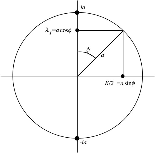
FIGURE 3. The $\lambda$-plane in the inverse scattering transform for solutions of the NLS equation. This is the spectral domain in which homoclinic breathers live. Here the eigenvalue ${\lambda }_i$ lies on the interval between the origin and the carrier (0, ia).

Assume $\Omega t+\gamma =\Omega \left(t+\gamma /\Omega \right)=\Omega \tau$, where $\tau =\left(t+\gamma /\Omega \right)$, we find

$u\left(x,\tau \right)=a\left(\frac{1-2\cos \left(Kx\right)e^{\Omega \tau -2i\varphi }+A{e}^{2\Omega \tau -4i\varphi }}{1-2\cos \left(Kx\right)e^{\Omega \tau }+A{e}^{2\Omega \tau }}\right)e^{2i{a}^{2}t}(31)$

Thus the parameter $\gamma$ introduces only a temporal phase shift that can be removed.

The most general form for the homoclinic solution below the carrier is then given by:

$u\left(x,t\right)=a\left[\frac{1-2e^{\gamma -2i\varphi +2a^2\sin \left(2\varphi \right)t}\cos \left(2a\sin \varphi x\right)+{\sec }^2\varphi e^{2\gamma -4i\varphi +4a^2\sin \left(2\varphi \right)t}}{1-2e^{\gamma +2a^2\sin \left(2\varphi \right)t}\cos \left(2a\sin \varphi x\right)+{\sec }^2\varphi e^{2\gamma +4a^2\sin \left(2\varphi \right)t}}\right]e^{2i{a}^{2}t}(32)$

Note that ϕ is the IST phase and γ is seen in the role of an amplitude-multiplying factor in the initial modulation. Now use

$\theta \left(t\right)=2a^2\sin \left(2\varphi \right)t(33)$

The primordial time is given by the following (set $\epsilon =e^{2a^2\sin 2\varphi t}$, then expand as a Taylor series in ε as $t\to -\infty$):

$u\left(x,t\right)\simeq a\left[1+4\epsilon e^{\gamma }\sin \varphi e^{i\left(\frac{\pi }{2}-\varphi \right)}\cos \left(2a\sin \varphi x\right)\right]e^{2i{a}^{2}t}(34)$

This corresponds to a small-amplitude modulation back at the “initial” time or initial condition where the motion is generated. Equation 34 is useful as an initial condition for the motion of a wave maker in a laboratory experiment. The subsequent wave motion evolves into a breather train as the waves propagate down the wave tank.

The higher genus solutions of the NLS equation found by Matveev and colleagues [36][37] correspond to the case $N=4$, and have a four-by-four Riemann matrix. Similar solutions have been developed by [15]. I will address these “multi component” solutions in detail with relation to the periodic IST in a later paper. These solutions are very important because they constitute homoclinic “superbreathers” in the solutions of the NLS equation.

It is worthwhile noting that the generalized homoclinic solutions of the NLS equation are wonderful in their own right and can be easily applied to problems in the physics of nonlinear wave propagation, to engineering, etc. However, when we analyze complex oceanic time series we are generally faced with hundreds or thousands of nonlinear modes. Thus the methods of Fourier analysis from inverse scattering theory must be applied to obtain the full nonlinear spectrum. In the case where the time series is described by a “rogue sea” then most of the energy in the spectrum will be “clustered” about the peak of the spectrum, and these modes consequently will be homoclinic. This means that we can combine generalized homoclinic solutions with the breather modes from time series analysis using the Zakharov-Shabat eigenvalue problem.

The Akhmediev Breather Solution

To obtain the Akhmediev breather we set ${\lambda }_I=ia/\sqrt{2}$ where

$\varphi =\frac{\pi }{4},\gamma =\frac{1}{2}\ln \left(\frac{1}{2}\right)(35)$

Equation 32 then reduces to the Akhmediev breather [16]:

$u\left(x,t\right)=-ia\left[\frac{\cos \left(\sqrt{2}a x\right) \text{sech}\left(2a^{2}t\right)+\sqrt{2}i \text{tanh}\left(2a^{2}t\right)}{\sqrt{2}-\cos \left(\sqrt{2}a x\right)\text{sech}\left(2a^{2}t\right)}\right]e^{2i{a}^{2}t}(36)$

The primordial form is given by as $t\to -\infty$:

$u\left(x,t\right)\simeq -ia\left[1+\sqrt{2}\epsilon \left(1+i\right)\cos \left(\sqrt{2}ax\right)\right]e^{2i{a}^{2}t}(37)$

This is the small amplitude Cauchy initial condition for a particular solution. The factor $-i$ is an arbitrary, non-physical, phase shift for the NLS equation, give by $-\pi /2$.

The Extreme Freak Wave

The largest wave happens for $\varphi \sim \Delta \varphi <<1$, which occurs at $x=t=0$, hence we compute from Eq. 32:

$\left|u\left(\mathrm{0,0}\right)\right|\left(\varphi ,\gamma \right)=\sqrt{1+\frac{4e^{\gamma }{\sin }^{2}2\varphi }{1+2e^{2\gamma }-4e^{\gamma }{\cos }^2\varphi +\cos 2\varphi }}(38)$

A graph of this function is given in Figure 4: $\left|u\left(\mathrm{0,0}\right)\right|\left(\varphi ,\gamma \right)$ as a function of $\varphi ,\gamma$. The maximum value is found at $\gamma =0$

$\left|\psi \left(\mathrm{0,0}\right)\right|\left(\varphi ,0\right)=\sqrt{5+4\cos 2\varphi }(39)$

FIGURE 4

FIGURE 4. Graph of the rogue wave maximum, $u_{\max }=\left|u\left(\mathrm{0,0}\right)\right|\left(\varphi ,\gamma \right)$, as a function of $\varphi ,\gamma$.

This is shown in Figure 5. Note that the maximum value occurs at the coordinate values $\gamma =\varphi =0$. Furthermore, an important observation is that Eq. 32 is indeterminate for $\varphi =0$. This singularity occurs for the Peregrine breather, where the maximum amplitude is 3 and therefore we hereafter assume $\varphi >0$.

FIGURE 5

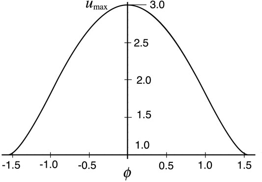
FIGURE 5. Graph of the largest freak waves as a function of the parameter $\varphi$, $u_{\max }=\left|\psi \left(\mathrm{0,0}\right)\right|\left(\varphi ,0\right)$, for $\gamma =0$.

The Peregrine Breather

The Peregrine breather happens in the limit that the spatial periodicity tends to infinity $L\to \infty$, at the same time the wavenumber tends to 0. The infinite period limit occurs for $\varphi \to 0$. We then obtain

$u\left(x,\tau \right)=a\left[\frac{1-2e^{-2i\varphi +2a^2\sin \left(2\varphi \right)\tau }\cos (2a\sin \varphi x)+{\sec }^2\varphi e^{-4i\varphi +4a^2\sin \left(2\varphi \right)\tau }}{1-2e^{2a^2\sin \left(2\varphi \right)\tau }\cos (2a\sin \varphi x)+{\sec }^2\varphi e^{4a^2\sin \left(2\varphi \right)\tau }}\right]e^{2i{a}^{2}t}(40)$

Here we have used

$\tau =\left(t+\frac{\gamma }{\Omega }\right)=\left(t+\frac{\gamma }{2a^2\sin (2\varphi )}\right)=t+{\gamma }_o(41)$

The shift in time occurs on both $\gamma$ and $\varphi$:

${\gamma }_o=\frac{\gamma }{2a^2\sin \left(2\varphi \right)}(42)$

For the limit $\gamma \to 0$ we can expand both the denominator and numerator to second order in $\varphi$. After simplifying we get the standard form for the Peregrine breather:

$u\left(x,t\right)=a\left[1-\frac{4\left(1+4{\mathrm{ia}}^{2}t\right)}{1+16a^4{t}^2+4a^2{x}^2}\right]e^{2i{a}^{2}t}(43)$

The Kuznetsov-Ma Breather

We now look at the plane region which lies above the carrier, as depicted in Figure 6. Therefore Eq. 6 becomes (use $\lambda =i{\lambda }_I$, $ia\le {\lambda }_I<\infty$, and ${\lambda }_I=a\cos \left(i\varphi \right)=a\cosh \varphi$):

$K\to 2\sqrt{a^2+{\lambda }^2}=2i\sqrt{{\lambda }_I^2-a^2}=2ia\sinh \varphi (44)$

This means further:

$\Omega \to K\sqrt{4a^2-K^2}=2i{a}^2\sinh \left(2\varphi \right)(45)$

We make the following transformation $\varphi \to i\varphi$, $K\to iK$ and $\Omega \to i\Omega$ to obtain the solution above the carrier in the lambda plane. This solution corresponds to a large amplitude modulation:

$u\left(x,t\right)=-ia\left(\frac{1-2\cosh \left(Kx\right)e^{i\Omega t+2\varphi +\gamma }+A{e}^{2i\Omega t+4\varphi +2\gamma }}{1-2\cosh \left(Kx\right)e^{i\Omega t+\gamma }+A{e}^{2i\Omega t+2\gamma }}\right)e^{2i{a}^{2}t}(46)$

The Kuznetsov-Ma breather [18], [14] occurs for ${\lambda }_I=ia\sqrt{2}$ and is given by:

$u(x,t)=a\left[1+\frac{2\left(\cos \left[4\sqrt{2}{a}^{2}t\right]+i\sqrt{2}\sin \left[4\sqrt{2}{a}^{2}t\right]\right)}{\cos \left[4\sqrt{2}{a}^{2}t\right]+\sqrt{2}\cosh \left[2ax\right]}\right]e^{2i{a}^{2}t}(47)$

The maximum value of the Kuznetsov-Ma waveform is $u_{\max }\left(0,\pi /\left(4\sqrt{2}{a}^2\right)\right)=1+2\sqrt{2}\cong \mathrm{3.828.}$ The period in time T is given by

$T=\frac{\pi }{2\sqrt{2}{a}^2}(48)$

We now consider the interval $\left(-\pi /\left(2\sqrt{2}{a}^2\right),0\right)$ in time, where the initial waveform occurs, leading to a:

$u\left(x,t\right)=a\left[1+\frac{2}{1+\sqrt{2}\cosh \left[2ax\right]}\right]e^{2i{a}^{2}t}(49)$

For $a=1,x=0$ we see that this large amplitude initial condition has amplitude 1.828. In a wave tank experiment we thus have a large amplitude initial condition for all waves with spectral parameters above the carrier. This contrasts to the cases below the carrier, which have small amplitude initial conditions.

FIGURE 6

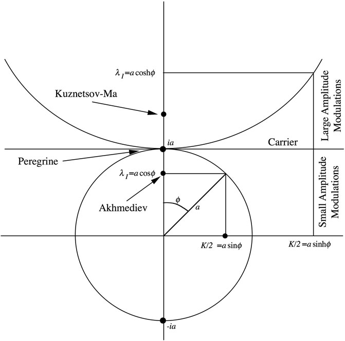
FIGURE 6. Parameters for the homoclinic solution of the NLS equation above the carrier in the lambda plane, i.e., where ${\lambda }_I$ can be seen to lie on the interval $\left(ia,i\infty \right)$. This diagram makes clear the regions of small-amplitude modulations below the carrier and the region of large-amplitude modulations above the carrier.

Comments on Data Analysis

We have seen how the homoclinic solutions of the NLS equation are constructed and further how these reduce to the particular forms for the Akhmediev, Peregrine and Kuznetsov-Ma breathers. The general formula for the homoclinic solution Eqs 20–24 describes a single nonlinear Fourier component of the inverse scattering method for some complete “potential” of the NLS equation. This statement means: Given a space or time series that describes an energetic sea state in which there are many large breather packets, each packet is then approximately homoclinic and is therefore given in the space/time domain by Eqs 20–24. This provides a simple alternative to Riemann theta functions to describe, in an experimental context, the actual space/time dynamics of each breather train in the nonlinear spectrum in the absence of the other breathers. Consequently one can think of the homoclinic breather Eqs 20–24 as a simple road to an approximate filtering algorithm in which single breathers can be extracted from a measured wave train and then subsequently graphed as a single component. We now give an experimental overview of how one then interprets the spectrum for a particular time series.

Structure of the Nonlinear Spectrum

One strong point of the nonlinear Fourier analysis approach is that the solutions of the nonlinear wave equations are given very generally by Riemann theta functions. This means that one can “least squares fit” theta functions to measured time series to determine the Riemann spectral parameters, essentially in a fashion similar to that for ordinary periodic Fourier analysis. In the present case however one solves the Floquet problem for the Zakharov-Shabat eigenvalue problem to determine the spectral parameters [5]. The nonlinear parameters to be determined include the Riemann matrix, frequencies and phases of the nonlinear spectral components. Nonlinear Fourier analysis has coherent structures, so that the data can be analyzed in terms of Stokes waves, solitons, breathers and superbreathers. The Stokes waves constitute the diagonal elements of the Riemann matrix and the off-diagonal elements are the nonlinear interactions. The Stokes waves may be small enough that they are essentially sine waves, or they may be so large that they form solitons. If the Stokes waves are large enough (such that the Benjamin-Feir parameter is greater than 1), they nonlinearly couple or phase lock to each other to become breathers. This perspective contrasts with the usual assumption that ocean waves consist of weakly interacting sine waves, which we now know is valid only for very small ocean waves [5]. In modern times, however, we have the option of using nonlinear Fourier analysis to describe ocean waves as they really are, i.e., as huge numbers of nonlinearly interacting coherent structures.

Understanding the full physical behavior of coherent structures on the many aspects of ocean wave dynamics therefore plays an important role in modern research. The influence of coherency on wind wave modeling, data analysis, and computation of wave forces on ships and offshore structures are some of the reasons for improving our knowledge of the nonlinear dynamics of ocean waves with coherent structures.

It is worthwhile discussing briefly the structure of the spectrum of the NLS equation in deep-water ocean waves, primarily because deep water constitutes most (over 99%) of the ocean. In deep water the NLS equation coherent structure solutions consist of Stokes waves, (bright) soliton wave packets, breather wave trains and superbreathers. A typical ocean wave train in terms of these structures is given in Figure 7. This simple representation of a nonlinear spectrum has arisen from a large number of time series measurements and subsequent analysis by nonlinear Fourier methods [5], [11], [12]. Thus we see in Figure 7 a nonlinear spectrum that is generated by wind on waves in a generic fashion: The shape of the spectrum consists of nonlinear wave components that are solutions of the NLS equation that are generated by Mother Nature in the real world environment. To interpret the spectrum it is worthwhile noting that the larger the spectral components are the more nonlinear they are. The larger components generally occur about the peak of the spectrum. The continuous black line in Figure 7 is a typical ocean wave spectrum such as that described by the Pierson-Moskowitz or JONSWAP power spectra. The points (black and red dots) are the components of the nonlinear ocean wave spectrum. The dots are “points of simple spectrum” from the Zakharov-Shabat eigenvalue problem [38]. The larger the components are, the greater is the nonlinearity.

FIGURE 7

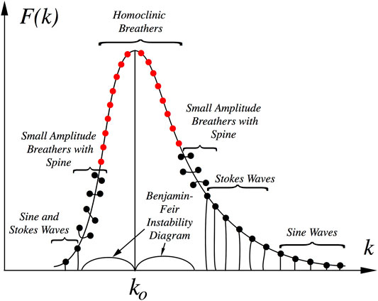
FIGURE 7. Schematic of typical nonlinear wavenumber spectrum for deep-water ocean waves. For a large amplitude sea state the spectral energy is dominated by the largest breathers, which are essentially homoclinic (red dots).

Referring to Figure 7 the character of the nonlinear components is given by a mathematical object called a spine, which is a line of spectrum that either descends to the frequency axis from a point of spectrum, or connects two points of simple spectrum above the frequency axis. The components with spines that descend to the frequency axis are sine or Stokes waves. The low amplitude tails of the spectrum typically contains small-amplitude sine waves while slightly larger components (slightly nearer the peak of the spectrum) are Stokes waves. The frequency band about the peak of the spectrum has the components that are most nonlinear: Here the spines are seen to connect two points of simple spectrum, corresponding to small or medium amplitude breathers. The red dots are “double points”, i.e., two points of simple spectrum that nearly coincide and thus the spines are too short to be visible: These are the homoclinic breathers in the spectrum. In a large sea state these homoclinic breathers are clustered about the spectral peak and energetically dominate the nonlinear wave motion [39], [12]. Sea states of densely packed breathers are referred to as “breather turbulence” and consequently characterize a “rogue sea” condition.

The double lobed curves, shown at the bottom of the graph on the frequency axis, are centered about the peak of the spectrum at the carrier wavenumber $k_o$. This double lobe constitutes the “instability diagram” of the Benjamin-Feir instability region: Spectral points within this band of spectrum are breathers. Once again the red dots are the homoclinic breathers. They are the biggest and baddest of the breather packets and are sources of rogue waves in the sea state. When the largest breather packets reach their maximum amplitudes during their breathing cycles the central wave is often viewed as a rogue wave. The wave trains that characterize the nonlinear waves for each red dot are the homoclinic solutions of Eqs 20–24 discussed above in this paper. Therefore, for anyone wanting to study nonlinear waves these homoclinic solutions can be very important for a full understanding of the most energetic coherent structures in the spectrum, i.e., those that are sources of rogue waves in a “rogue sea.” Breathers consist of two phase locked Stokes waves with a 2 × 2 Riemann spectrum and we see they have a homoclinic limit, Eqs 20–24. Superbreathers consist of three or four (or more) phase locked Stokes waves and they too have a homoclinic limit. Up to now breathers are ubiquitous spectral components in measured ocean wave time series [40], [11], [12]. Superbreathers have yet to be found in ocean wave measurements up to now.

How can a spectrum of wind waves of the type shown in Figure 7 be generated by wind in the ocean? Beginning with a calm sea state the wind starts to blow and the initial small amplitude waves have the form of a random sea state that has a rough spectral shape similar to the solid curve in Figure 7. At this stage it is found that the nonlinear wave components are essentially sine waves. After the wind brings up the sea state slightly more we find the spectrum consists of sine waves that interact weakly with one another. Further injection of wind energy into the sea state we find that the nonlinear components near the peak of the spectrum become Stokes waves. Further energy input forces couples of Stokes waves near the peak to phase lock with each other creating breather trains. For a fully “nonlinearly saturated” sea state most of the energy near the peak of the spectrum is dominated by breather trains. We have found that in Currituck Sound the breathers are quite dense and 30-min time series have over 200 breathers, suggesting that “breather turbulence” might be a proper way to describe these types of energetic sea states which might also be called “rogue seas.”

It might be tempting to try and describe ocean waves in terms of a few simple breather trains and it would seem reasonable to think of large breathers as rare events. However, for ocean waves it has been found that for extreme sea states the breathers are highly dense and each breather has its own shape and dynamical properties. For example their maximum heights are random statistical variables, and so to are their rise times. Thus breathers as nonlinear Fourier modes are drastically different from simple weakly interacting sine waves. It is also worthwhile noting that while the nonlinear Schrödinger equation has many complex types of nonlinear Fourier modes, it is unclear how those modes might be distributed in a particular physical situation. Only through experimental measurements and their subsequent analysis by nonlinear Fourier analysis, can we begin to understand the true physical behavior of nonlinear ocean waves and what their nonlinear spectra are. We now understand that the old paradigm of weakly interacting sine waves is no longer tenable. However, the full consequences of large sea states dominated by coherent structures are still to be fully understood. The implications of such a new scenario on all aspects of living and working in the ocean will only slowly become better understood as the new paradigm is exploited to better understand nonlinear stochastic wave motion with coherent structures.

Fossil Breathers and Ghost Packets in Shallow Water

We would like to briefly discuss the possible existence of “fossil” breathers in shallow water. What are these special solutions of the shallow water NLS equation? Suppose that one has a deep-water breather that is propagating toward shore over decreasing water depth. At some point it will pass the depth where $Kh=1.363$ and the breather train will no longer be Benjamin-Feir unstable. What happens physically to the breather packet if it is placed in shallow water, where the sign of the nonlinear terms of NLS equation changes? One still, momentarily, has a wave packet that has essentially the same shape as the precursor deep-water breather. However, in shallow water the packet now has a real frequency, not the imaginary frequency for BF unstable dynamics in deep water. This new shallow water packet, still phase locked as in the deep-water case, will therefore propagate shoreward with a fixed shape, i.e., it no longer breathes. The packet will undergo wave transformation (changes in shape) as it propagates into even shallower water. Under the right conditions each of the large waves in the packet will roll over and break and possibly create good conditions for surfing. We call this shallow water packet (before roll over and breaking) a “fossil” breather because it contains in its nonlinear Fourier parameters all the information necessary to compute the properties of the original breather back in “primordial” time far offshore, perhaps even in terms of a far away storm. Thus shallow water measurements of fossil breathers should provide understanding of the incoming flux of breathers from deep water. The fossil breathers are “ghosts” of the past breathers, which are now dead and gone once the BF instability no longer dominates their dynamics. Figuratively speaking their breathing has been switched off at the transition from deep to shallow water, at $Kh=1.363$, where they effectively die and propagate shoreward as ghost breathers out of the past. Theoretically the simplest way to understand how this happens is to study the theta function solution of the NLS equation for the case $N=2$, the topic of a future paper.

Conclusion

A discussion of the general homoclinic solutions of the 1+1 NLS equation is given and a several ways to derive them are discussed. This work sets the stage for using the homoclinic solution to help analyze and understand experimental data from laboratory and oceanic measurements of nonlinear waves. Analysis of space/time series data using the Zakharov-Shabat eigenvalue problem are given elsewhere. What has been found in these data analyses is that for high amplitude sea states the spectrum is energetically dominated by breather states that are very nearly in the homoclinic limit. This experimentally determined idea then provides motivation for this paper in which we treat the homoclinic spectral components as being represented by Eqs 20–24, expressions which are valid for any mode anywhere in the lambda plane. This provides a heuristic interpretation of experimental data for energetic sea states as being a linear superposition of homoclinic breathers plus interactions amongst these breathers. Such an interpretation suggests that new filtering procedures could be used to extract individual breather modes from time series. Details of the application of this procedure to data will be given in future papers.

Data Availability Statement

The original contributions presented in the study are included in the article/supplementary material, further inquiries can be directed to the corresponding author.

Author Contributions

The author confirms being the sole contributor of this work and has approved it for publication.

Funding

This work has been supported by Tom Drake of the Office of Naval Research of the United States.

Conflict of Interest

Author AO was employed by the company Nonlinear Waves Research Corporation.

Publisher’s Note

All claims expressed in this article are solely those of the authors and do not necessarily represent those of their affiliated organizations, or those of the publisher, the editors and the reviewers. Any product that may be evaluated in this article, or claim that may be made by its manufacturer, is not guaranteed or endorsed by the publisher.

Acknowledgments

The author thanks the referees for their positive comments.

Footnotes

¹Associated with the Floquet problem for the Zakharov-Shabat eigenvalue problem.

References

1. Akhmediev N, Pelinovsky E. Discussion and Debate: Rogue Waves – towards a Unifying Concept?. Eur Phys J Spec Top (2010) 185(Issue 1). doi:10.1140/epjst/e2010-01233-0

CrossRef Full Text | Google Scholar

2. Kharif C, Pelinovsky E, Slunyaev A. Rogue Waves in the Ocean. Berlin: Springer-Verlag (2009).

Google Scholar

3. Olagnon M, Athanassoulis GA. Rogue Waves 2000. Brest: Ifremer (2000).

Google Scholar

4. Olagnon M, Prevost M. Rogue Waves 2008. Brest: Ifremer (2008).

Google Scholar

5. Osborne AR. Rogue Waves: Classification, Measurement and Data Analysis, and Hyperfast Numerical Modeling. Eur Phys J Spec Top (2010) 185:225–45. doi:10.1140/epjst/e2010-01251-x

CrossRef Full Text | Google Scholar

6. Pelinovsky E, Kharif C. Extreme Ocean Waves. Berlin: Springer-Verlag (2008).

Google Scholar

7. Kotljarov VP, Its AR. Dopovidi Akad Nauk UkRSR., Ser A (1976) 11:965–8.

8. Tracy ER, Chen HH. Nonlinear Self-Modulation: An Exactly Solvable Model. Phys Rev A (1988) 37:815–39. doi:10.1103/physreva.37.815

CrossRef Full Text | Google Scholar

9. Belokolos ED, Bobenko AI, Enolskii VZ, Its AR, Matveev VB. Algebro- Geometric Approach to Nonlinear Integrable Equations. Berlin: Springer-Verlag (1994).

Google Scholar

10. Lamb GL. Elements of Soliton Theory. New York: John Wiley & Sons (1980).

Google Scholar

11. Costa A, Osborne AR, Resio DT, Alessio S, Chirivì E, Saggese E, et al. Soliton Turbulence in Shallow Water Ocean Surface Waves. PRL (2014) 113:108501. doi:10.1103/physrevlett.113.108501

CrossRef Full Text | Google Scholar

12. Osborne AR, Resio DT, Costa A, Ponce de León S, Chirivì E. Highly Nonlinear Wind Waves in Currituck Sound: Dense Breather Turbulence in Random Ocean Waves. Ocean Dyn (2018) 69:187–219. doi:10.1007/s10236-018-1232-y

CrossRef Full Text | Google Scholar

13. Osborne AR. Nonlinear Fourier Analysis: Rogue Waves in Numerical Modeling and Data Analysis. J Mar Sci Eng (2020). in press. doi:10.1115/omae2020-18850

CrossRef Full Text | Google Scholar

14. Ma Y-C. The Perturbed Plane-Wave Solutions of the Cubic Schrödinger Equation. Stud Appl Math (1979) 60:43–58. doi:10.1002/sapm197960143

CrossRef Full Text | Google Scholar

15. Ablowitz MJ, Clarkson PA. Solitons, Nonlinear Evolution Equations and Inverse Scattering. Cambridge: Cambridge University Press (1991). doi:10.1017/cbo9780511623998

CrossRef Full Text | Google Scholar

16. Akhmediev N. Teoreticheskaya I Matematicheskaya Fizika (1986) 69(2):189–94.

17. Peregrine DH. Water Waves, Nonlinear Schrödinger Equations and Their Solutions. J Aust Math Soc Ser B, Appl. Math (1983) 25:16–43. doi:10.1017/s0334270000003891

CrossRef Full Text | Google Scholar

18. Kuznetsov E. Solitons in a Parametrically Unstable Plasma. Sov Phys Dokl (1977) 22:507–8.

Google Scholar

19. Toffoli A, Onorato M, Bitner-Gregersen EM, Monbaliu J. Development of a bimodal structure in ocean wave spectra. J Geophys Res Oceans (2010) 115:C03006.

CrossRef Full Text | Google Scholar

20. Toffoli A, Bitner-Gregersen EM, Osborne AR, Serio M, Monbaliu J, Onorato M. Extreme Waves in Random Crossing Seas: Laboratory Experiments and Numerical Simulations. Geophys Res Lett (2011) 38:L06605.

CrossRef Full Text | Google Scholar

21. Chabchoub A, Hoffmann NP, Akhmediev N. Rogue Wave Observation in a Water Wave Tank. Phys Rev Lett (2011) 106:204502. doi:10.1103/physrevlett.106.204502

PubMed Abstract | CrossRef Full Text | Google Scholar

22. Islas AL, Schober CM. Predicting Rogue Waves in Random Oceanic Sea States. Phys Fluids (2005) 17:031701. doi:10.1063/1.1872093

CrossRef Full Text | Google Scholar

23. Pinho UF, Babanin AV. Emergence of Short Crestedness in Originally Unidirectional Nonlinear Waves. Geophys Res Lett (2015) 42:4110–5.

CrossRef Full Text | Google Scholar

24. Mozumi K, Waseda T, Chabchoub A. 3D Stereo Imaging of Abnormal Waves in a Wave basin. In ASME 2015 34th International Conference on Ocean, Offshore and Arctic Engineering. New York: Am Soc Mechanical Engineers (2015) (Accessed May 31, 2015). doi:10.1115/omae2015-42318

CrossRef Full Text | Google Scholar

25. Sanina EV, Suslov SA, Chalikov D, Babanin AV. Detection and Analysis of Coherent Groups in Three-Dimensional Fully-Nonlinear Potential Wave fields. Ocean Model (2016) 103:73–86. doi:10.1016/j.ocemod.2015.09.012

CrossRef Full Text | Google Scholar

26. Chabchoub A, Mozumi K, Hoffmann N, Babanin AV, Toffoli A, Steer JN, et al. Directional Soliton and Breather Beams. Proc Natl Acad Sci U S A (2019) 116(20):9759–63. doi:10.1073/pnas.1821970116

PubMed Abstract | CrossRef Full Text | Google Scholar

27. Abramowitz M, Stegun IA, 55. United States: National Bureau of Standards, Applied Mathematics Series, U.S. Dept. of Commerce (1964). Handbook of Mathematical Functions

Google Scholar

28. Dysthe KB. Note on a Modification to the Nonlinear Schrödinger Equation for Application to Deep Water Waves. Proc R Soc Lond A (1979) 369(–114).

Google Scholar

29. Trulsen K, Dysthe KB. A Modified Nonlinear Schrödinger Equation for Broader Bandwidth Gravity Waves on Deep Water. Wave Motion (1996) 24:281–9. doi:10.1016/s0165-2125(96)00020-0

CrossRef Full Text | Google Scholar

30. Zakharov VE. Stability of Periodic Waves of Finite Amplitude on the Surface of a Deep Fluid. J Appl Mech Tech Phys USSR (1968) 2:190.

Google Scholar

31. Yuen HC, Lake BM. Nonlinear Dynamics of Deep-Water Gravity Waves. Adv Appl Mech (1982) 22:67–229. doi:10.1016/s0065-2156(08)70066-8

CrossRef Full Text | Google Scholar

32. Hirota R. “Direct Methods in Soliton Theory,” in Solitons RK Bullough, and PJ Caudry, editors, 17. Berlin-Heidelberg-New York: Springer-Verlag (1980). p. 157–176. doi:10.1007/978-3-642-81448-8_5

CrossRef Full Text | Google Scholar

33. Hirota R. Exact Envelope‐soliton Solutions of a Nonlinear Wave Equation. J Math Phys (1973) 14:805–9. doi:10.1063/1.1666399

CrossRef Full Text | Google Scholar

34. Herbst BM, Ablowitz MJ. Numerically Induced Chaos in the Nonlinear Schrödinger Equation. Phys Rev Lett (1989) 62:2065–8. doi:10.1103/physrevlett.62.2065

PubMed Abstract | CrossRef Full Text | Google Scholar

35 Osborne AR. Classification of Homoclinic Rogue Wave Solutions of the Nonlinear Schrödinger Equation. Nat Hazards Earth Syst Sci Discuss 2 (2014). 897–933.

Google Scholar

36. Dubard P, Gaillard P, Klein C, Matveev VB. On Multi-Rogue Wave Solutions of the NLS Equation and Positon Solutions of the KdV Equation. Eur Phys J Spec Top (2010) 185:247–58. doi:10.1140/epjst/e2010-01252-9

CrossRef Full Text | Google Scholar

37. Dubard P, Matveev VB. Multi-rogue Waves Solutions to the Focusing NLS Equation and the KP-I Equation. Nat Hazards Earth Syst Sci (2011) 11:667–72. doi:10.5194/nhess-11-667-2011

CrossRef Full Text | Google Scholar

38. Osborne AR. Deterministic and Wind/Wave Modeling: A Comprehensive Approach to Deterministic and Probabilistic Descriptions of Ocean Waves. In Proceedings of the 31st International Conference on Ocean, Offshore and Arctic Engineering OMAE2012 June 10-15. Rio de Janeiro, Brazil (2012).

CrossRef Full Text | Google Scholar

39. Osborne AR. Advances in Nonlinear Waves with Emphasis on Aspects for Ship Design and Wave Forensics. In Proceedings of the ASME 2013 32nd International Conference on Ocean, Offshore and Arctic Engineering OMAE2013 June 9-14. France: Nantes (2013). doi:10.1115/omae2013-10873

CrossRef Full Text | Google Scholar

40. Osborne AR, Nonlinear Ocean Waves and the Inverse Scattering Transform. Acad Press, Int Geophys Ser 97 (2010). p. 944.

Google Scholar