A Stochastic Model Based on Fiber Breakage and Matrix Creep for the Stress-Rupture Failure of Unidirectional Continuous Fiber Composites 2. Non-linear Matrix Creep Effects

Introduction

From a materials engineering perspective, stress rupture (sometimes called creep-rupture) is a time-dependent failure mode in unidirectional, continuous fiber composites that are primarily loaded in tension over long time periods and whose failure is typically catastrophic. Such composites, often consisting of carbon fibers in an epoxy matrix, operate at either ambient temperatures, or temperatures well below the matrix glass transition temperature. Examples of such structures include composite overwrapped pressure vessels (COPVs), tension members in infrastructure applications such as cables in suspended roofs, post-tensioned bridge platform cables, and rotors spinning at high angular velocity such flywheels, centrifuges and propellers, where hoop and radial stresses become very large. In such cases, stress rupture failure is explosive resulting in sudden release of potential and/or kinetic energy and in the case of COPVs the stored contents can also be combustible. Typically, stress-rupture occurs with little or no warning, and its unpredictable nature necessitates large safety factors even when a considerable experimental data base exists to support various life prediction methodologies.

In engineering applications, which are often subject to life-safety requirements, much of the concern stems from the fact that reliabilities in such structures must be extremely high (e.g., probability of failure <10⁻⁸) over a specified lifetime (typically many years) under a specified service load. No amount of brute-force testing can directly demonstrate such reliabilities, especially when test objects in the laboratory necessarily differ from actual service components in key respects, such as being much smaller in overall material volume under load. Thus, size effects are a key issue, and predicting stress-rupture lifetime, and particularly the lower tail of the lifetime distribution for a given load, inevitably requires sophisticated modeling in light of any previous, or simultaneously generated, test data.

The general experimental approach to characterizing the stress-rupture behavior of such a carbon fiber/epoxy structures in applications is to first determine the strength distribution of subscale artifacts, such as epoxy-impregnated strands, or small laboratory scale pressure vessels, which have been filament wound using the same materials. Typically, a Weibull strength distribution is observed, and the Weibull scale and shape parameter values are estimated. Then several fixed stress levels are selected, and for each level multiple test artifacts are placed under test and failures recorded over time, which in many cases requires many months and sometime years to gather sufficient lifetime data for prediction purposes. Typically, the lifetime data is also found to be of Weibull form, but with extremely high variability (low Weibull shape parameter value typically less than unity). Furthermore, statistical estimation techniques, such as maximum likelihood, must be used to deal with censored test samples, since at lower stress levels, only a few of the test samples may have failed.

While methods vary for analyzing and presenting such strength and stress-rupture data, the general approach is often to plot the mean lifetime (or Weibull lifetime scale parameter) vs. fixed stress level on log-stress vs. log-lifetime coordinates, and to fit a power law, i.e., lifetime varies as stress level to a negative power, which is often of the order of 100 in magnitude. Some effort may also be made to estimate the shape parameter for Weibull lifetime at each stress level, hopefully the same for each, and from the results, to determine a stress level that results in the desired high reliability, i.e., low probability of failure over the chosen structural component lifetime.

The previously mentioned approaches to modeling stress-rupture lifetime are discussed in detail in [1–4] where it is shown that such a lifetime estimation approach is fraught with many serious difficulties some of which are as follows: First, there are serious practical limitations in sample sizes that can be tested at each stress level. Second, since the variability in lifetime is very high, the uncertainty in any reliability estimate is also very high to the point of resulting in unusable reliability bounds (much less providing the ability to select between competing models, which are typically phenomenological). Third, the typically used “proof test” approach to screen out weaker, and presumably, lower reliability specimens is fraught with difficulties, such as what proof stress level to use, and whether damage is caused to the structure in the act of proof testing that cancels any potential benefit, perhaps even making the structure even less reliable. Thus there is a need for the development of sophisticated models that consider the micromechanics and statistics of fiber load-sharing and failure, and which are reasonably tractable and whose predictions can be defended. Since we are most interested in the high reliability (low probability of failure) region of various distributions, we are able to take advantage of various power-law approximations to the lower tails of various Weibull distributions to construct reliability estimates. This is seen throughout the derivations.

Before developing the model, and in view of the broad audience, we provide some context regarding the breadth of fiber bundle models that have played a key role in the study of failure processes in a heterogeneous materials, as conducted in statistical physics, materials, and mechanics communities. Some excellent reviews from various perspectives are provided in [5–10]. The simplest versions focus on material strength in response to an applied load, and where individual fibers are assumed to have variability in their strengths following some probability distribution, such as uniform or Weibull, the latter being common to engineering applications [9, 10]. Under a tensile bundle load some fibers fail, and their loads are transferred to their survivors, some of which may also fail due to their increased loads, leading to more load redistribution, and so on. Depending on applied bundle load, the bundle may either reach a stable state where some smaller group of surviving fibers are strong enough to support the bundle load, or, all survivors are exhausted and the bundle collapses. As discussed below, details on the evolution of this failure process depend on the bundle load magnitude, the fiber strength distribution, the bundle size (number of fibers), and critically on the mechanism by which fibers share and redistribute load.

In the simplest bundle models, load-sharing mechanisms fall between two extremes: (i) equal load-sharing (ELS) where the loads of failed fibers are redistributed equally onto all survivors, and (ii) local load sharing (LLS), where the loads of failed fibers are transferred onto their closest surviving neighbors, as expanded upon in [5–10]. Under ELS fiber failure patterns tend to be diffuse and percolation-like, whereas under LLS, clusters of breaks nucleate and grow reminiscent of catastrophic cracks. The contrast in the two pattern types depends on the variability in fiber strength. Larger variability results in increasingly similar failure patterns across the load redistribution range from ELS and LLS, however, that the bundle strength statistics ultimately differ as bundle size grows indefinitely, as shown in [9, 10].

In statistical physics, various aspects are of interest, such as critical behavior, recursive failure dynamics, universality classes, burst distributions and avalanches, precursors (warnings) of global failure, cross-over behavior, and localization in terms of forming of critical clusters vs. mean field analysis [5–8]. In both the physics and engineering communities size effects are a key issue [9–13] because the size scales of multiple laboratory test samples are necessarily orders of magnitude smaller than their monolithic structural counterparts in applications. Approaches to the study of such models vary from being purely analytical (requiring various simplifying assumptions but yielding profound insight) to numerical Monte Carlo methods where fiber strengths and load redistribution for evolving failure configurations are directly calculated. Numerical simulation has limitations, however, because bundle structures of interest can have more than 10⁸ fiber elements (e.g., carbon fiber/epoxy composite overwrapped pressure vessels) whereas eventual scaling behavior may be inconclusive in bundles of 10⁴ to 10⁵fiber elements, and require 10³replications to obtain accurate statistics. Additionally, while some researchers use mean field approaches, attempting to calculate the limiting strength of bundles approaching infinite size, others focus on obtaining distributions for strength of finite-size bundles especially deep into their lower tails particularly when high reliability is of concern. For instance finding a particular bundle load for which the failure probability is <10^−ℵ may be of interest, where ℵ ≥ 8 (sometimes referred to as the “number of nines” of the reliability, 1 − 10^−ℵ) would require at least 10^ℵ+1 = 10⁹ replications, currently a computationally prohibitive number. How to extend to such low probability levels for large-scale structures such as carbon-fiber/epoxy pressure vessels is a key challenge and is where theoretical modeling and scaling arguments become powerful tools, as is addressed in this paper.

Generalizations of simple fiber bundle models for material strength, particularly for longer structures, typically assume fiber flaw occurrence along an individual fiber following a compound Poisson point process in distance and flaw strength (local failure stress). When the flaw strength follows a power law, the result is a Weibull distribution for fiber strength vs. length that satisfies weakest link statistics. We call this a Weibull-Poisson (WP) fiber strength model. For long bundles with fibers bonded together in a flexible matrix, or in a stiff matrix but where the matrix has a low yield strength or the fiber-matrix interface is weak and slip occurs, ELS generalizes to global load-sharing (GLS). Under GLS a fiber can fail at multiple locations along its length, however, at any cross-sectional composite plane, a locally failed fiber may still carry some load depending on the distance from the plane to its closest break. In cases where LLS still applies at a cross-section, behavior also depends on whether the bundle is planar (i.e., each fiber has only two flanking neighbors) or the fibers are packed in a square, hexagonal or random array in which case failing fibers have many neighbors onto which to redistribute their loads. Thus, milder versions of LLS emerge at a plane where some load is transferred to next-nearest and even further neighbors following some power-law decay in lateral distance. In both GLS and LLS failure tends to concentrate in transverse planes whereby material failure is well-described using a chain-of-bundles approach [9, 13], which means that size effects become important [11–13].

The failure of heterogeneous materials typically involves time-dependence of some form, and in accommodating such features, fiber bundle models become more complex, but also richer in features, as can be seen in [14–55]. Time dependence can enter into the bundle failure process in various ways: First, the fiber breakdown process may be thermally activated as for instance in [14–29], or may involve time-dependent kinetics of flaw growth in the fiber as in [30, 31]. On the other hand, the matrix may creep, or the fiber/matrix interface may slip over time, thus causing relaxation in broken fibers and overloading of others [32–55], thus altering the length scale of fiber-to-fiber load transfer.

In the case of the former where fiber load-sharing, ranging from ELS to LLS, is by itself time independent, many models for time-dependent fiber failure involve a breakdown rule with the fiber failure rate depending on fiber stress level raised to a power, or as an exponential in fiber stress level. These rules are often tied to activation energy ideas of molecular bond failure, depending on the absolute temperature. In such cases, the fiber lifetime distribution under fixed load may be taken as exponential (constant hazard rate over time) and in others, a memory integral of past stress history is involved. This integral then becomes the argument of a second function controlling the shape of the lifetime distribution, and when of power form and the fiber is under a constant stress, Weibull fiber lifetime results. Several works specifically focus on such time-dependent fiber bundles as well as more elaborate network and lattice extensions, a sampling of which are discussed in [14–29]. In papers involving varying ranges of lateral load transfer somewhere between the ELS and LLS extremes, crossovers from mean-field to short range behavior are seen where break clusters form and instability is seen. To span ELS to LLS, the degree of localization also depends on the magnitude of the power-law breakdown exponent. Even in LLS bundles, one may see ELS-like diffuse fiber failure when the power-paw exponent approaches two and especially below 1 as shown in [24–27].

The works [14–29], which span the last 25 years of research, reveal surprising consistency in the overall behavior observed, in terms of size effects, localization in cluster growth and the types of lifetime distributions obtained, especially in the lower tails. Numerical Monte Carlo methods have become more efficient and computational power has increased, for a bundle with a given geometric and load-sharing complexity, by two to three orders of magnitude in size, which has been critical to providing insight into ultimate convergent (or divergent) behavior as the size scale increases. Fortunately, analytical models with various idealizations based on LLS and GLS modeling approaches have proven very effective in uncovering characteristics of bundle lifetime distributions deep into their lower tails. In cases where a clear choice between an LLS vs. a GLS modeling approach is ambiguous, it often happens that the two approaches result in surprisingly similar lifetime distribution shapes.

Other bundle models with time-dependent fibers (or analogs at the molecular scale) involve unique approaches [32–34] to specialized circumstances. For instance [32], which models a metal-matrix composite, involves a creeping, elasto-plastic matrix, and fibers that have some mix of strength behavior and time dependent degradation, all treated in a finite-element framework. Another approaches fiber behavior using a kinetic Monte-Carlo algorithm based directly on thermal fluctuations [33]. In another, fibers constitute a molecular network and a molecular dynamics approach is used [34].

Yet another group of models [35–37], involve fibers that are essentially elastic but upon failure undergo slow relaxation behaving as Maxwell elements. In [35], the fiber strength follows a uniform distribution and the modeling is purely GLS with broken fibers slowly shedding load to their survivors. In [36] fiber strengths are assumed Weibull a with shape parameter of two, whereupon bundle lifetime was found to be lognormal. In [37] the load-sharing ranged between GLS and LLS using a power-law, variable range of interaction rule, and again Weibull fiber strength. The two universality classes associated with GLS vs. LLS extremes appeared robust.

The focus in the current paper is on time-dependent bundle models where the fibers are brittle, initially continuous, time-independent, and that are aligned in a polymer matrix that itself supports negligible tensile load. The fibers have WP strength properties and time dependence enters through matrix shear creep around fiber breaks, which over time increases the length-scale of fiber load transfer at breaks. Examples of models in an ELS-GLS framework are described in [38–41], where in [38–40] plots of stress level vs. the logarithm of the mean lifetime is of interest, whereas in [41] the interest is on the residual composite strength after considerable time spent under constant load. These models do not focus on the nature of the lifetime distribution over time given the applied stress level. Of particular interest are such bundle models under LLS, several of which are discussed in [42–55]. The first two models [42, 43] are predecessors to the model we develop later and involve both theory and experiments on the strength and creep-rupture of seven-fiber, micro-composites of carbon fibers in an epoxy. They demonstrate various features of interest in the current paper, including Weibull fiber strength, distributions for micro-composite strength with Weibull “envelopes” having segments predicted by LLS theory, Weibull lifetime distributions also having Weibull envelope segments, and lastly, plots of log-load vs. log-lifetime behavior whose slopes depend on the shape parameter for fiber strength and the power-law creep exponent in time. Also, [44] contains a supporting analytical/numerical model for composite creep-rupture involving Weibull fibers with planar and hexagonal fiber packing in a linearly viscoelastic matrix.

Two related works [45, 46], present both theory and experimental results on the strength and lifetime of epoxy-impregnated carbon fiber strands. The models, however, are largely phenomenological and do not directly build on micromechanical LLS behavior with matrix creep. Nonetheless, such microstructural behavior arguably underlies the behavior observed. Time-dependence is reflected in the epoxy creep compliance, including time-temperature shift factors. This framework provides coherence to both the strength and the lifetime distributions obtained, respectively, at various strain rates and fixed stress levels, and at temperatures from 298°K to 443°K. Strand strength followed a Weibull distribution, and lifetime distributions were shown where the scale parameter had log-log dependence through a function of normalized time based on the matrix creep response. Overall, the experimental behavior seen is consistent with the model results we develop later.

In a sequence of papers by Bunsell et al. [47–55], a model has been developed that considers the lifetime of unidirectional carbon fiber-epoxy composites under sustained loads, and where the main application is filament wound pressure vessels. In [47] the work begins with numerical modeling of the micro-mechanisms of fiber-to-fiber load transfer resulting from WP fiber failures. In [48], the load-transfer mechanism over time is altered by relaxation due to the viscoelastic and plastic behavior of the matrix, also causing locally increasing loads on neighboring fibers. In larger scale structures, these processes are used in [49] to model fiber break progression in a multi-scale framework, involving representative volume elements (RVEs) applicable to both strength and lifetime testing. In the latter, delayed fiber failures occur as new flaws are exposed thus leading to growing fiber break clusters and their coalescence into a critical damage state causing composite failure. Their model is applied in [50] to carbon fiber-epoxy matrix pressure vessels where the issue of proof testing is raised, and where the authors comment as follows:

“At present, there are no proof testing techniques or in-service reliability assessments techniques, which are mentioned in standards that are suitable or based on the failure processes known to control lifetimes of composite structures.”

Later in the same paragraph, the authors say:

“A hydraulic [proof] test on a composite pressure vessel has only one clear outcome, which is that fibers, which ordinarily would not have broken, fail during the test and the vessel is closer to failure than it was before the test, as is illustrated in Figure 2.”

Much of their work in [50] is directed at determining an appropriate proof test level, for both new pressure vessels and pressure vessels that have seen pressurized service over long time periods. Investigating the issue of proof-testing is also a primary focus in the model we develop later.

In later works [51–55], these authors extend their RVE modeling in terms of the formation and evolution of small clusters of breaks called of i-plets of various sizes (e.g., two-plets, four-plets, eight-plets, 16-plets, 32-plets, …). The focus is on critical damage states in tension testing [51], sustained loading over time [52], and laminated structures [53]. The work in [54, 55] looks deeper into critical damage states in terms of i-plets as precursors to imminent failure and on the possibility of determining a lower threshold for applied composite stress below which the lifetime becomes infinite [55]. Overall, the impressive multi-scale model developed in [47–55] is computationally intensive so that Monte Carlo replications beyond a few 100 samples are currently impractical. Except in [55] where 100 replications were performed, the focus was largely on mean lifetime behavior, rather than the form of lifetime distributions, particularly in their lower tails. Nonetheless the overall failure process is qualitatively very similar to that which we develop later, and thus, some of our results may be of use in extending their models in [47–55].

As with many models described previously, a key assumption in the model we develop later is that individual carbon fibers are time independent, that is, essentially immune from creep rupture at typical temperatures of interest. This has been established in the work of Farquhar et al. [56]. A second assumption is that the mechanics of fiber stress-relaxation and load transfer around fiber breaks is accurately described by a non-linear matrix creep law, including a matrix plastic-like yielding effect. Over the past two decades there have been many papers [57–62], that have used micro-Raman spectroscopy and other techniques to measure time-dependent stress-relaxation and load transfer around fiber breaks in arrays of carbon fibers in an epoxy matrix. These experiments have been interpreted using sophisticated shear-lag modeling in [59–62] assuming elastic fibers and a linearly viscoelastic matrix, and which reveal the occurrence of varying degrees of shear yielding and debonding at the fiber-matrix interface, particularly at fiber strains approaching fiber failure. Thus, the assumption of a linearly elastic-perfectly bonded matrix requires revision, as will be key in our modeling approach in later sections. Indeed, there are several theoretical works [63–67] that allow us to make such revisions.

Our model involves the growth of clusters of fiber breaks to critical size. The concept of critical cluster formation under LLS has been a feature of various models discussed earlier. In this work we draw heavily on the mechanics of fiber load transfer around breaks as pioneered in the work of Hedgepeth and NASA associates [68–70]. The clusters in our model are idealized as growing in a planar fashion, whereas one might expect fiber breaks to be staggered out of plane. However, near planar cluster growth is often seen [71], and in effect clusters act as though they are increasingly planar as the length scale of load transfer increases over time [44]. We especially note a body of work [9, 10, 44, 72–76] specifically devoted to growth of clusters of fiber breaks to critical size, and the associated probability calculations through analysis and Monte Carlo simulation. Actual clusters seen in Monte Carlo simulations over time often have a far more random shape than the idealized clusters we consider. However, despite their differing appearance, upon reaching catastrophic instability the resulting failure distributions are remarkably similar to the point where only a small scaling adjustment is necessary to create congruence deep into the lower distribution tails. This behavior holds up even for Weibull shape parameters in the range of 2 or 3, which is below those for carbon fibers of interest in this paper. A group of recent papers [74–76] is very insightful regarding the nature of the critical cluster concept in LLS, and the limited role played by local ELS behavior within small groups of fiber failures but embedded within an overall LLS framework, and resulting distributions shapes and size scaling. These findings are remarkable and when experiment does not match theory, one may better focus more broadly on variability introduced in fabrication of a structure, rather than just on shortcomings in modeling assumptions. For instance, in [77] various fiber packings were considered including square, hexagonal and random, and yet the results proved surprisingly robust. Similar robust behavior was noted in [26, 27] working with distorted triangular lattices. Such details are less important that might first be suspected, which perhaps explains why fiber bundle models, with all their idealizations, work so well in the first place.

The focus of this paper, therefore, is to revisit and further develop our previous model [78] that took into account not only the statistical failure of individual fiber elements in the composite, but also linearly viscoelastic matrix behavior in shear as the matrix locally transfers loads from broken fibers elements to neighboring intact fiber elements over a length-scale that increases over time.

As was described above in the context of a wide range of fiber bundle models, stress rupture is caused by fiber breakage occurring over time, where individual fiber breaks ultimately form clusters that increase in size until one becomes unstable and the composite fails catastrophically. A key aspect is that the load once carried by a broken fiber is locally transferred to its neighboring fibers through shear in the matrix, thus creating stress concentrations in these neighbors, which then grow in time especially as fiber breaks form in clusters that grow. A key driver of the failure process is that the local length-scale of these overloads increases over time as the matrix creeps in shear so that, over time, more and more fiber flaws are exposed to stresses that cause them to fail, despite having survived the applied service load absent any stress-concentrations, or even loads from a proof test. Thus, a critical aspect of this stress-rupture process occurring in the composite over time, is that it occurs even if the fibers themselves are immune to stress-rupture, which is essentially the case for carbon fibers.

The stress rupture failure process described above is the basis for the stochastic fiber breakage (SFB) model [78], which accounts for the relevant micromechanics of fiber-to-fiber load transfer in the presence of matrix creep, and the statistics of fiber strength and flaw occurrence in determining the overall lifetime distribution. Several other models have been applied to describe stress-rupture composite lifetimes; however, these models have largely been phenomenologically based on single fibers, as described in [14–19, 79], some of which are compared in [1]. In developing the micro-mechanically based SFB model in [78], many simplifying assumptions were necessary.

One key assumption was that the matrix is linearly viscoelastic, and creeps in shear following a power-law in time. This assumption has been used in shear-lag modeling [63–65] and mathematically builds on models assuming elastic fibers and an elastic matrix. Associated with this assumption, however, is that the matrix and the fiber/matrix interface are immune to failure in shear, which may be an unrealistic assumption when fiber breaks first occur, or clusters become large. Of course, over time, matrix creep relaxes these initially high shear stresses, however, it is known that in many circumstances of high fiber volume fraction and fiber strength the initial shear stresses around fiber breaks exceed the matrix yield strength or interfacial shear strength for fiber-matrix debonding. The SFB model in [78] does not accommodate such non-linear matrix phenomena, although qualitatively and using rough approximations, their consequences can be appreciated as significant when they occur. Thus, to accommodate such non-linear matrix behavior in shear, Mason et al. [66] investigated the case where the matrix undergoes non-linear creep in shear, both in stress and time. The current paper extends the SFB by incorporating the non-linear results in [66] into our previous model in [78].

Lastly, we discuss the effect of proof testing on composite lifetime in this revised version of the SFB model with non-linear matrix behavior, and how the additional parameters that arise allow us to accommodate non-linear matrix behavior such as plastic-like matrix yielding, yet preserve the overall character of the results.

Section Overview of Context of the Stochastic Fiber Breakage Model and Forms of Key Results provides a brief overview of the context of the SFB model in applications as well as various distribution forms that will expanded upon in subsequent sections. Section Modeling the Instantaneous Composite Strength and Determining its Distribution provides a derivation of the distribution for “short-term” composite strength, in circumstances where the timescale for matrix creep is assumed too short to affect the strength behavior, as was the case in [78]. However, certain parameters will be defined in anticipation of non-linear matrix effects that will require revisions to the model of [78].

Section Modeling Composite Lifetime in Stress Rupture and Determining its Distribution derives the distribution for composite lifetime, building on the methods used in Section Modeling the Instantaneous Composite Strength and Determining its Distribution and previously in [78], but also incorporating non-linear viscoelastic behavior to the matrix, using a variation of the load transfer length explored in [66] and expanded upon in Appendices A–D (All Appendices are provided in the Supplementary Material linked to the paper). In Appendix A, context is provided for how various parameters arise and the roles they play, particularly with respect to the growth in time of the characteristic load-transfer length. Appendices B,C derive results accommodating shear-driven increases in the length scale of load-transfer on surviving fibers around a growing cluster of fiber breaks. In Appendix D we discuss a simpler version of the non-linear creep model in [66], which is analytically solvable for all the 3-fiber cases in Appendix A, including those where the exponent on time is not unity. The behavior of crucial quantities, such as the length scale of fiber load transfer over time, turn out to be virtually identical.

Section Lifetime Distribution of a Composite Component that has Survived a Proof Test derives the distribution for lifetime of a composite component that has survived an initial proof-test up to some fraction of its initial strength (or has been overloaded by some multiplier of its ultimate service stress). Section Results and Discussion summarizes the influence of non-linear matrix creep on various parameters governing the distributions for composite strength and lifetime, and illustrates various results and non-linear effects in graphical form where the effects of varying certain key parameters are discussed, paying special attention to more subtle volume effects.

Section Conclusions concludes with some comments on key distinguishing features of the model that result from extending into the non-linear range the viscoelastic matrix creep behavior in our previous work [78]. We also provide some additional context on the overall stress-rupture problem in unidirectional composite structures that goes beyond the task of developing a model, as was done in this paper.

Overview of Context of the Stochastic Fiber Breakage Model and Forms of Key Results

Load Profiles Applied to the Composite and Desired Strength and Lifetime Distributions

Ramp Loading to Determine Composite Strength

The first load history of interest is the ramp loading for determining the composite strength. This is given by:

$\begin{array}{ll}\sigma (t)=Rt,t\ge 0& (1)\end{array}$

where t is time and the parameter, R > 0, is the loading rate or stress rate. Typically, R is sufficiently fast to cause failure in 20–200 s, and where such failure times are shorter than a particular characteristic time, t_c, for matrix creep in shear, especially the fraction of time spent closer the failure load where most fiber breakage occurs. As such, the time-dependence of the matrix is typically ignored when modeling composite strength behavior, and we can treat the matrix as though it is purely elastic (though there will be exceptions and subtleties worthy of discussion).

In this case, the goal is to calculate the distribution function, H_V(σ), for the strength of the composite, in terms of applied stress level, σ > 0, which will turn out to be approximately of Weibull form with scale and shape parameters, ${\widehat{\sigma }}_V$ and $\widehat{\alpha }$, respectively, that are to be determined from the model and where V is the composite volume expressed as the total number of fiber elements it contains, each with characteristic length, δ_c. Note that applied stress is to be interpreted as applied force divided by some overall fiber material cross-sectional area of the structure, and will not the same as the elevated local stress on a particular fiber element that happens to be next to a newly broken fiber element, and thus, is also supporting part of that fiber element's original load.

Constant Load in the Study of Composite Stress-Rupture Lifetime

The second load history of interest is that used in modeling composite lifetime in stress rupture. In this case, applied stress is assumed to be constant over all time, i.e.,

$\begin{array}{ll}\sigma (t)=\bar{\sigma },t\ge 0& (2)\end{array}$

where $\bar{\sigma }>0$ is the applied stress level (fiber force over overall fiber material cross-sectional area of the loaded structure), and in practice, is typically only a fraction of the Weibull scale parameter for composite strength measured using the ramp loading (1), that is, $\bar{\sigma }<{\widehat{\sigma }}_V$. In reality, the initial loading of the composite up to stress level, $\bar{\sigma }$, cannot be performed instantaneously and typically requires an initial ramp loading following load-history (1), where R is sufficiently rapid. However, time-dependence of the matrix under such initial loading rates, typically has a negligible effect on the resulting lifetime distribution at times of interest well-beyond the characteristic time, t_c, mentioned above. Note that this applied stress can only be supported as long as the elevated local fiber stresses near some growing cluster of fiber breaks in the material, have not reached the point where cluster growth becomes unstable and catastrophic.

In this case, the goal is to calculate the distribution function, $H_V(t;\bar{\sigma })$, for the lifetime of the composite, for times, t ≫ t_c, which will also be of the Weibull form with scale and shape parameters, ${\widehat{t}}_V$ and $\widehat{\beta }$, respectively, and where V is the previously defined composite volume. We will find that ${\widehat{t}}_V=t_{\mathrm{\text{c}}}{\left(\bar{\sigma }/{\widehat{\sigma }}_V\right)}^{-\widehat{\rho }}$ where $\widehat{\rho }$ is a power-law exponent that will characterize the dependence of the lifetime on the inverse of the applied stress level, $\bar{\sigma }$.

Stress-Rupture Lifetime of a Composite Following a Brief Proof Test at Higher Load

Typically manufactured composite structural components, prior to being put into service, are subjected to a “proof test” where a ramp loading (1), is applied up to proof stress level, σ_p, which may be significantly higher than the ultimate service stress, $\bar{\sigma }$, and which is maintained for some proof hold time, t_p, typically several minutes, after which the applied stress is lowered to the service stress level, $\bar{\sigma }\le {\sigma }_{\mathrm{\text{p}}}$, which is kept constant thereafter (Here we admit the possibility that the proof test is minimal, i.e., the stress level is simply the ultimate service stress). There can be variations to this loading profile whereby after time, t_p, the applied stress is lowered from σ_p to near zero and the component is stored for some time before later being put into service at constant stress $\bar{\sigma }$. For the purposes of this paper, however, it suffices to use the simplified load profile:

$\begin{array}{ll}\sigma (t)=\{\begin{array}{ll}{\sigma }_{\text{p}},& 0\le t<t_{\text{p}}\\ \bar{\sigma },& t\ge t_{\text{p}}\end{array}& (3)\end{array}$

The rationale for this practice is that applying a proof test to stress level, ${\sigma }_{\mathrm{\text{p}}}\ge \bar{\sigma }$, will “weed out” inferior composite structural components, thus improving the overall reliability of components that pass the proof test and are put in service. As is discussed later, classic models used for composite lifetime in stress rupture typically support this strategy, and the higher the proof stress, the better. We shall show, however, that the more detailed model developed in this paper does not universally support such a strategy, since proof-testing inflicts damage in the form of broken fibers that otherwise would have remained intact. This can negatively influence composite reliability at much longer times. This is a critical issue raised by Bunsell and Thionnet [50], as previously mentioned.

In this case we are interested in the conditional distribution for lifetime, $H_V\left(t|t\ge t_{\mathrm{\text{p}}},{\sigma }_{\mathrm{\text{p}}},\bar{\sigma }\right)$, given t ≥ t_p, that is, given the component survived the proof test loading under stress σ_p up to time t = t_p, which means $H_V\left(t|t\ge t_{\mathrm{\text{p}}},{\sigma }_{\mathrm{\text{p}}},\bar{\sigma }\right)=0$ when t = t_p. The resulting lifetime distribution has a complex but insightful structure, though it does not neatly collapse to a Weibull form, even when ${\sigma }_{\mathrm{\text{p}}}=\bar{\sigma }$.

Modeling the Instantaneous Composite Strength and Determining Its Distribution

Distribution for Fiber Strength in Tension and Size (Length) Effect

Fibers in the composite are initially continuous having diameter, d, and Young's modulus, E. We assume the WP fiber strength model applies, such that a fiber element of length, δ, follows a Weibull distribution for tensile strength, σ, of the form:

$\begin{array}{ll}{F}_{\delta }(\sigma )=1-exp\left(-\frac{\delta }{{\delta }_{\text{c}}}{\left(\frac{\sigma }{{\sigma }_{{\delta }_{\text{c}}}}\right)}^{\zeta }\right),\sigma \ge 0& (4)\end{array}$

where δ_c is a characteristic length mentioned earlier and described in more detail below, and σ_δc and ζ are the fiber Weibull scale and shape parameters, respectively, corresponding to length δ_c. A critical feature of (4) is that increasing the element length, δ, increases the probability of element failure at stress level, σ, since more strength limiting and randomly occurring flaws are exposed. Note also that the Weibull scale parameter for fiber strength at length, δ, is simply:

$\begin{array}{ll}{\sigma }_{\delta }={\sigma }_{{\delta }_{\text{c}}}{({\delta }_{\text{c}}/\delta )}^{1/\zeta }& (5)\end{array}$

which reveals the inverse dependence of fiber strength on length, δ, and its sensitivity to ζ. This becomes a key component of the stress-rupture model for lifetime since matrix creep in shear has the effect of increasing over time, t, the effective overload lengths on fiber segments adjacent growing clusters of fiber breaks. However, the fibers and their randomly occurring flaws are themselves time independent, and segments of fixed length and under a fixed load do not undergo stress rupture.

A Taylor series expansion of (4) results in a convenient lower tail approximation, namely:

$\begin{array}{ll}{F}_{\delta }(\sigma )\approx \frac{\delta }{{\delta }_{\text{c}}}{\left(\frac{\sigma }{{\sigma }_{{\delta }_{\text{c}}}}\right)}^{\zeta },0\le \sigma <{\sigma }_{\delta },& (6)\end{array}$

which is of power-law form. This approximation happens to be extremely accurate for typical values of ζ, since fiber stress levels, σ, in the composite failure model typically satisfy 0 ≤ σ ≪ σ_δc. Later the composite stress-rupture model will involve the formation and growth of clusters of fiber breaks that have formed under an applied composite stress level, σ. Intact neighbors next to a cluster of i fiber breaks will thus be subject to stress K_iσ > 1, where K_i is the fiber stress concentration induced by the cluster (as will be described in more detail in sub-section Stress Concentrations and Break Cluster Growth Parameters for Failing Fiber Elements below). If the cluster grows in size such that [[Mathtype-mtef1-eqn-77.mtf]], then under (6), F_δ(K_iσ) → 1, whereas under (4), F_δ(K_iσ) → 0.632 > 1/2. Either way, the fiber break cluster has reached instability and catastrophic failure results. However, (6) greatly simplifies the calculations.

Characteristic Elastic and Statistical Length Scales for Fiber Load Redistribution Near Breaks

Using the classic shear-lag model [68, 69], Hedgepeth et al. described the load transfer process from broken to intact fibers in a composite where fibers are arranged in either a planar, square or hexagonal array within a flexible matrix. Fundamentally, a characteristic elastic length, δ_e, emerges that depends on various mechanical and geometric parameters of the fiber and matrix and their spacing, these being the fiber Young's modulus, E, fiber cross-sectional area, A, fiber diameter, d, matrix instantaneous elastic shear modulus, G_e, effective width, w, of matrix between two fiber surfaces, and the effective matrix thickness, which is also taken as d.

For fully elastic behavior, δ_e is typically expressed in terms of these parameters as [9, 63–65]:

$\begin{array}{ll}{\delta }_{\text{e}}=d\sqrt{\frac{E}{G_{\text{e}}}\frac{A}{d^2}\frac{w}{d}}\approx d\sqrt{\frac{E}{G_{\text{e}}}\frac{w}{d}}& (7)\end{array}$

the latter assuming the approximation A ≈ d², The dominating influences on δ_e are the fiber diameter, d, the square root of the fiber to matrix stiffness ratio, $\sqrt{E/G_{\mathrm{\text{e}}}}$, and the square root of the matrix width between the fibers divided by its thickness $\sqrt{w/d}$. In simple terms, the ratio w/d is related to the fiber volume fraction, V_f, and whether the fibers are arranged as a planar tape (planar fiber array) or as a hexagonal array, whereby V_f ≈ 1/(1 + κw/d) where κ ≈ 2 for a planar fiber array and κ ≈ 3 for a hexagonal array. Thus, for a given fiber volume fraction, the ratio w/d will be smaller for a hexagonal vs. a planar array, however, the effect is mitigated by the square-root since $\sqrt{2/3}=0.816$, and thus, for a given V_f the effect on δ_e is no more than 20%.

Along a neighboring fiber close to a fiber break, its overload profile in terms of fiber stress is roughly triangular with the peak stress occurring adjacent to the break. However, the effect of the triangular stress profile, in terms of determining its probability of failure can be modeled using an “effective, rectangular overload profile” at peak stress, but over some shorter length depending on the Weibull shape parameter, ζ, for fiber strength. This calculation requires accounting for the statistical rate of occurrence along the fiber of flaws of varying strength, as characterized by the WP fiber strength model [9, 10]. In our earlier work [78], this characteristic length, called δ_c in (4) through (6), was chosen as ${\widehat{\delta }}_{\mathrm{\text{c}}}$, which in our current notation and under linear viscoelastic behavior in [78] is:

$\begin{array}{ll}{\widehat{\delta }}_{\text{c}}\equiv \frac{4}{\zeta +1}{\delta }_{\text{e}}.& (8)\end{array}$

One factor of “2” arises because the overload profile extends over length 2δ_e spanning the break. The other factor, 2/(ζ + 1), arises from triangular nature of the over-stress profile and its integration within the WP fiber model over length 2δ_e [For more details see Equations (85–88) in [9] and associated discussion there]. The scaling factor, which is inversely proportional to ζ + 1, results from the fact that the higher the value of ζ, the lower the variability in fiber strength, which means there is a sparser distribution of weaker flaws along the fiber. Thus, only the higher stresses near the peak of the triangular overload region are likely to cause fiber failure. Overall, the overloaded region is shortened for larger values of ζ [We caution that the notation used here is different from that in [78], since 2δ_e here is ${\widehat{\delta }}_{\mathrm{\text{e}}}$ in the previous paper where both sides of the break were included. The definition of δ_e in (7) is more in line with that in the literature, [9, 10, 68, 69], and will simplify later comparisons].

In the current work the introduction of non-linear creep, and in particular, effects associated with the applied composite stress level, will require modification of δ_c, and we will find that taking ${\delta }_{\mathrm{\text{c}}}={\widehat{\delta }}_{\mathrm{\text{c}}}\equiv 4{\delta }_{\mathrm{\text{e}}}/(\zeta +1)$, as in [78], does not account for the matrix yielding effect that will need to be incorporated. A new form of δ_c will be developed in Section Modeling Composite Lifetime in Stress Rupture and Determining its Distribution Fiber-to-Fiber Load Transfer at Fiber Breaks Under Linear and Non-linear Matrix Creep in Shear and in Appendix A in the Supplementary Material once the non-linear matrix creep model has been introduced, and a scale parameter for composite strength has been formulated; however, in this section δ_c needs no further characterization.

Stress Concentrations and Break Cluster Growth Parameters for Failing Fiber Elements

In the absence of time dependence of the matrix, the failure process in the composite involves the growth of clusters of fiber breaks resulting from local stress local concentrations on intact neighbors that are candidates for the next fibers to fail. Thus, in accordance with the definitions in both [10] and [78], we let:

$\begin{array}{cc}{K}_i=\{\begin{array}{c}\sqrt{1+i\pi /4},\text{ planar fiber array,}\\ \sqrt{1+\sqrt{4i/\pi }/\pi },\text{ hexagonal fiber array,}\end{array}i=0,1,2,\dots & (9)\end{array}$

be the stress concentration on a fiber next to a cluster of i broken fibers, where we note that $\sqrt{4i/\pi }=D$, is the diameter (dimensionless) of an approximately disc-shaped cluster containing i tightly-packed fiber breaks (That is, the actual cluster diameter is of order Dd). Also,

$\begin{array}{ll}{c}_k={\displaystyle \prod _{j=0}^{k-1}}{N}_j,k=1,2,3,\dots & (10)\end{array}$

is approximately the number of ways a cluster of k breaks can grow one break at a time from a single triggering break, where N₀ ≡ 1 and N_j is the effective number of overloaded neighbors next to a cluster of size j, one of which becomes the next fiber failure. The number, N_j, is given in [10, 44, 78] as approximately,

$\begin{array}{ll}{N}_j=\{\begin{array}{l}2,\text{ planar fiber array}\\ \varphi j^{\gamma },\text{ hexagonal fiber array }\end{array},j=1,2,3,\dots & (11)\end{array}$

where in a hexagonal array, ϕ and γ are parameters having the respective ranges, 2.5 ≤ ϕ ≤ 6 and 0 ≤ γ ≤ 0.5 depending on subtleties of the fiber packing geometry and other factors. These all apply to the case of a linearly viscoelastic matrix.

In Appendix C in the Supplementary Material we consider the effects of non-linear matrix creep behavior of the matrix in shear on the overload lengths of fibers next to a cluster of breaks of size j, and find that the definitions of N_j change in both cases, and in a hexagonal array γ can increase by as much as 1/2 depending on the degree of non-linearity in shear stress level. These aspects will be explored in terms of determining N_j in (11) and calculating c_k in (10) when applying the model in Section Results and Discussion.

Distribution Function for Composite Strength

In determining the probability of composite failure as a function of stress level, σ, under a ramp loading as described in (1), we first focus on a quantity W_k(σ), which is the probability of a cluster of k fiber breaks forming at a particular location in the composite under arbitrary stress, σ, starting with a single fiber break, and where k ≥ 1 is an arbitrary integer. These results are used later in connection with a specific value of $k=\widehat{k}$, called the critical cluster size for instability. Any group of k adjacent fiber elements has the potential to become a cluster of k breaks, despite being a rare event for a given group of k fibers. However, the probability of obtaining at least one cluster of size k somewhere in the composite is much larger, and the overall probability of occurrence takes the weakest link form:

$\begin{array}{ll}{H}_{V,k}(\sigma )=1-{\left[1-W_k(\sigma )\right]}^V,\sigma \ge 0,k=1,2,3,\dots & (12)\end{array}$

where V is the dimensionless volume of the composite in terms of number of fiber elements of length δ_c, That is, V, is the total length of fiber in the composite, Λ, divided by δ_c. Note that (12) holds even though two nearby groups of k fiber elements can overlap each other and might ostensibly be viewed as statistically dependent. In reality, they satisfy the concept of k-dependence and essentially act independently (see Smith et al. for theorems on the concept of k-dependence associated with rare events [72]].

Since V is large (12), is well-approximated by the exponential form:

$\begin{array}{ll}{H}_{V,k}(\sigma )\approx 1-exp\left[-V{W}_k(\sigma )\right],\sigma \ge 0,& (13)\end{array}$

reminiscent of the Weibull form, as described by Smith et al. [72]. The general expression for the strength of a cluster of k fibers, W_k(σ), as described in [9, 10, 78], is well-approximated by:

$\begin{array}{ll}{W}_k(\sigma )\approx c_k\left[{\displaystyle \prod _{i=0}^{k-1}}{F}_{{\delta }_{\text{c}}}(K_i\sigma )\right],k=1,2,3,\dots ,\sigma \ge 0.& (14)\end{array}$

where F_δc(σ), K_i and c_k were given previously by (6) and (9–11), respectively.

Using the lower tail approximation in (6), we can rewrite (14) as:

$\begin{array}{ll}{W}_k(\sigma )\approx c_k{\left(K_0{K}_1{K}_2\cdots K_{k-1}\right)}^{\zeta }{\left(\frac{\sigma }{{\sigma }_{{\delta }_{\text{c}}}}\right)}^{k\zeta },k=1,2,3,4,\dots .& (15)\end{array}$

Combining Equations (13) and (15), and taking $k=\widehat{k}$, which is the critical cluster size whose value is determined below, we obtain an approximation for the failure probability of the composite, H_V(σ), at a stress level σ, where:

$\begin{array}{ll}{H}_V(\sigma )\equiv {H_{V,k}(\sigma )|}_{k=\widehat{k}}& (16)\end{array}$

This can be rearranged into the Weibull form:

$\begin{array}{ll}{H}_V(\sigma )\approx 1-exp\left(-{\left(\frac{\sigma }{{\widehat{\sigma }}_V}\right)}^{\widehat{\alpha }}\right),\sigma \ge 0,& (17)\end{array}$

Where,

$\begin{array}{ll}{\widehat{\sigma }}_V={\sigma }_{{\delta }_{\text{c}}}{\left(V{c}_{\widehat{k}}\right)}^{-1/\left(\widehat{k}\zeta \right)}{\left({\displaystyle \prod _{i=0}^{\widehat{k}-1}}{K}_i\right)}^{-1/\widehat{k}},\widehat{k}\ge 1,& (18)\end{array}$

is the effective Weibull scale parameter for strength and

$\begin{array}{ll}\widehat{\alpha }=\widehat{k}\zeta ,\widehat{k}\ge 1,& (19)\end{array}$

is the corresponding effective Weibull shape parameter.

In [78], we defined the critical cluster size, $\widehat{k}$, as the value $\bar{k}$ satisfying $K_{\bar{k}-1}{\widehat{\sigma }}_V<{\sigma }_{{\delta }_{\mathrm{\text{c}}}}\le K_{\bar{k}}{\widehat{\sigma }}_V$. The idea there is that at such composite stress level $\sigma ={\widehat{\sigma }}_V$, the probability of failure of an adjacent element to a cluster of size, of size $\bar{k}-1$ is approaching 1−e⁻¹ = 0.632 and adding one more break to increase the cluster to size $\bar{k}$ pushes the failure probability to the point of instability, and thus, catastrophic cluster growth with any further breaks.

For typical values of ζ, this choice works well in the case of a planar array, since there only two neighboring fibers to a growing cluster. However, in the case of a hexagonal array, the number of overloaded neighbors, N_j, to a cluster of size, j, grows large, especially for smaller ζ values. Thus, a point of instability for a given stress value σ, will likely occur at a smaller cluster size, $\widehat{k}$, than the $\bar{k}$ value above, that is, the true $\widehat{k}$ would be overestimated by the definition given in [78].

To address this issue, a more refined approach to determining the $\widehat{k}$ associated with the onset of cluster instability is to first seek stress values, σ = σ_k, for integer values, k ≥ 1, where W_k−1(σ) happens to intersect with W_k(σ) when σ is locally varied; that is, where W_k(σ_k) = W_k+1(σ_k). These intersections result in a set of stress values satisfying ··· < σ_k < σ_k−1 < ··· < σ₂ < σ₁ < σ_δc, thus placing the focus on the probabilities of instability and failure associated with a given stress level, σ, that happens to fall between two successive values, say, σ_k ≤ σ < σ_k−1. Thus, using (15) in the equality W_k(σ_k) = W_k+1(σ_k) and canceling common factors leads simply to $K_k{\sigma }_k={\sigma }_{{\delta }_{\mathrm{\text{c}}}}/N_k^{1/\zeta }$. Then for ${\widehat{\sigma }}_V$ satisfying ${\sigma }_k<{\widehat{\sigma }}_V\le {\sigma }_{k-1}$ for a particular k value that we call critical cluster size, $\widehat{k}$, we find that:

$\begin{array}{ll}{K}_{\widehat{k}-1}{\widehat{\sigma }}_V<\frac{{\sigma }_{{\delta }_{\text{c}}}}{N_{\widehat{k}}^{1/\zeta }}\le K_{\widehat{k}}{\widehat{\sigma }}_V.& (20)\end{array}$

Thus, this result adjusts for the increased probability of instability and failure resulting from a growing number, $N_{\widehat{k}}$, of overloaded neighbors to a cluster, any one of which could break and trigger unstable cluster growth before the stress on such neighbors has reached σ_δc (The exponent, 1/ζ arises from an equiprobability tradeoff of increasing N_k vs. decreasing stress level, σ, so that N_kσ^ζ remains fixed).

From (9), (18), and (20) we find that solving for the correct value of $\widehat{k}$ requires satisfying:

$\begin{array}{ll}\widehat{k}=\{\begin{array}{cc}\lceil \frac{4}{\pi }\left\{{\left(2^{-1/\zeta }{\sigma }_{{\delta }_{\text{c}}}/{\widehat{\sigma }}_V\right)}^2-1\right\}\rceil ,& \text{planar fiber array}\\ \lceil \frac{{\pi }^3}{4}{\left\{{\left(N_{\widehat{k}}^{-1/\zeta }{\sigma }_{{\delta }_{\text{c}}}/{\widehat{\sigma }}_V\right)}^2-1\right\}}^2\rceil ,& \text{hexagonal fiber array}\end{array}& (21)\end{array}$

where “⌈▪⌉” corresponds to the ceiling function, i.e., rounding up the value of the argument to the next integer, since instability requires growing to the next highest cluster size. While this change in definition decreases $\widehat{k}$ as compared to that calculated in [78], it has a negligible effect in the planar case for typical values of ζ. However, it results in a major improvement in the hexagonal case for smaller values of ζ, particularly since $N_{\widehat{k}}$ also rapidly decreases with decreasing $\widehat{k}$.

Note that the approach in the current paper results in a single Weibull distribution for strength for all stress levels and associated probabilities of failure, whereas a more refined analysis, as in [9, 10], leads to a strength distribution with a more concave shape in stress level noticeable over probability levels decreasing by many orders of magnitude (Later on, the same will be true of the distribution for lifetime given the applied load level). However, apart from greatly complicating the analysis, such refinements make little if any practical difference to the predictions for the material volumes and range of failure probabilities of interest.

Modeling Composite Lifetime in Stress Rupture and Determining Its Distribution

The fiber breakage model for stress-rupture of a unidirectional composite relies not only on the elastic stiffness properties of the fibers in tension, but also on the elastic stiffness and creep properties of the matrix in shear. The fiber and matrix viscoelastic or viscoplastic properties and their dimensions with respect to their local packing geometry (e.g., 2D hexagonal, or 1D planar) determine the length scale, generally called δ(t), t ≥ 0 (of with subscripts as appropriate), over which load is transferred from a broken fiber to its adjacent intact neighbors. It is the matrix creep behavior in shear, scaled by its elastic behavior, that determines how this length-scale of fiber load transfer grows over time, the consequence of which is the occurrence of additional fiber failures over time at newly exposed flaws. Thus, over time clusters of fiber breaks emerge and grow in both size and length of overloading until a point of instability is reached, and catastrophic failure is triggered. Below we explain how is determined in both the linear and non-linear matrix creep.

Length-Scales for Fiber Load Transfer Under Linear Viscoelastic Matrix Creep

Previously in [78] we considered the case where the matrix is linearly viscoelastic and that the matrix creeps in shear according to a creep compliance with the power-law form:

$\begin{array}{ll}J(t)=J_{\text{e}}\left(1+{\left(\frac{t}{t_{\text{c}}}\right)}^{\theta }\right),t\ge 0,& (22)\end{array}$

where J_e ≡ 1/G_e is the instantaneous elastic creep compliance (being the inverse of, G_e, the instantaneous elastic shear modulus), t_c, is a characteristic time for creep, and θ is a power-law exponent, all being positive in value. Generally, under a time varying shear stress, τ(s), t ≥ 0, the shear strain follows the convolution integral.

$\begin{array}{l}\gamma (t;\tau (\blacksquare ))={\displaystyle \underset{0}{\overset{t}{\int }}}J(t-s)\frac{d\tau (s)}{ds}ds\\ =\frac{1}{G_{\text{e}}}{\displaystyle \underset{0}{\overset{t}{\int }}}\left(1+{\left(\frac{t-s}{t_{\text{c}}}\right)}^{\theta }\right)\frac{d\tau (s)}{ds}ds& (23)\end{array}$

Under a given fixed shear stress, $\bar{\tau }$, the matrix shear strain is $\gamma (t,\bar{\tau })=\bar{\tau }J(t)$, and from (23) is,

$\begin{array}{l}\gamma (t,\bar{\tau })=\frac{\bar{\tau }}{G_{\text{e}}}\left(1+{\left(\frac{t}{t_{\text{c}}}\right)}^{\theta }\right)\\ \approx \frac{\bar{\tau }}{G_{\text{e}}}{\left(\frac{t}{t_{\text{c}}}\right)}^{\theta },t\gg t_{\text{c}}.& (24)\end{array}$

Typically t_c is of the order seconds to minutes, whereas the ultimate failure time of the composite in stress-rupture applications is of the order of months to years, and even many decades. Also, a typical value for a polymer matrix is θ ~ 0.25. In the case of a unidirectional composite with a large number of fibers, the stress redistribution from a broken fiber to its closest intact neighbors can be calculated using well-known shear-lag models, which assume the fibers primarily support tension and the much more flexible matrix primarily supports shear. In the case of the linear viscoelastic creep function for the matrix, and using the convolution (23), in an extensive analysis using Laplace transforms, Lagoudas et al. [63] showed that the length scale grows beyond the elastic length scale according to ${\delta }_{\mathrm{\text{e}}}\sqrt{1+{(t/t_{\mathrm{\text{c}}})}^{\theta }},t>0$, and thus the characteristic length scale is accurately described by:

$\begin{array}{ll}\delta (t)={\delta }_{\text{c}}\sqrt{1+{\left(\frac{t}{t_{\text{c}}}\right)}^{\theta }},t>0& (25)\end{array}$

where δ_c is the characteristic statistical-elastic length scale for instantaneous fiber load transfer given previously by (8), that is, in this special case of linear viscoelasticity, ${\delta }_{\mathrm{\text{c}}}={\widehat{\delta }}_{\mathrm{\text{c}}}$. Furthermore, the fiber stress concentrations, K_i, near clusters of i fiber breaks still follow (9), and as time passes, transversely somewhat misaligned breaks in a cluster act as though they are increasingly aligned [58].

At much longer times, t, relative to the characteristic time for creep, t = t_c, and in keeping with the approximation in (23) we simplify (24) to,

$\begin{array}{ll}\delta (t)\approx {\delta }_{\text{c}}{\left(\frac{t}{t_{\text{c}}}\right)}^{\theta /2},t_{\text{c}}\ll t,0<\theta \le 1& (26)\end{array}$

where we note that the exponent on normalized time has now become θ/2. This reduction by one-half of the effect of the matrix creep exponent on time, i.e., from θ to θ/2, occurs because matrix creep causes growth over time of the length-scale along a fiber over which stress-redistribution occurs as the fiber stress drops from the nominal far-field value, say σ, to zero at the break. Consequently, to maintain force balance in the fiber, the magnitude of the matrix shear stress necessarily diminishes with time, effectively slowing down the growth of matrix creep in shear compared to what one might deduce from (5).

Despite the reduction of the exponent, θ, in (24), to θ/2 in (26), this approximation accurately describes the behavior of (25) for longer times, t ≫ t_c, and at t = t_c gives the same value, δ_c, as (25) does at t = 0. Thus, when considering probabilities of failure associated very short times, or even when measuring strength at times, 0 < t ≪ t_c, accurate predictions are obtained from lifetime probability calculations based on using the simpler (26), and taking t = t_c, as we discuss again later.

A key feature of matrix creep is ignored in simply using (25) and (26), but is potentially important when a composite has an isolated break or a small break cluster, and the applied composite tensile stress suddenly increases or decreases at certain times, or, when the composite stress is constant but a small break cluster induces additional neighboring breaks at times t ≫ t_c, and grows in size, or some combination of the two. In such cases, the shear stress near fiber breaks can change substantially over time, and the amount of stress redistributed from broken to intact fibers, and the length scale over which it is applied, also changes over time in ways we model using (26) but not accounting for behavior implied by the stress history convolution (23). That said, the key elastic length-scale of load transfer, δ_e, for a single break or its counterpart for a small break cluster does not change (other than increasing slightly in a stepwise fashion as more breaks are added).

It turns out, however, that these result are surprisingly accurate even for the case of a viscous matrix where (26) applies exactly with θ = 1, and where the matrix viscosity is interpreted as t_cG_e [44, 64, 65]. Thus, despite these potential complications we are still able to use the forms (25) and (26) as well as the instantaneous load-redistribution factors, K_i, around fiber breaks obtained from elastic shear-lag analysis, as given in (9). That is, in the case of elastic fibers and a linearly viscoelastic matrix, these K_i happen to be determined from the elastic problem, via the so-called “correspondence principle.”

Thus, for all breaks, we assume (25) and (26) apply irrespective of when new breaks occurred; that is, the time of occurrence for any new break is retroactively set to zero. Since θ is typically small (and θ/2 smaller still), the effect of retroactively assigning all break times to zero, once they occur, makes little practical difference to the model predictions, which if anything are slightly conservative. Such a simplification yields surprisingly accurate predictions in a stress-rupture setting, as was shown in [54] for the more demanding case of a viscous matrix, θ = 1, especially when a composite is loaded under constant stress that is well below its breaking strength. Much of the reason for this is that the fiber breaking process, while rapid initially, becomes slower and slower as time progresses, and the spacing of breaks over time tends to become logarithmic, until catastrophic instability is reached. Consequently, log-scales in both time and stress level are typically used to describe the composite stress rupture process up to final failure.

Length Scales for Fiber Load Transfer Under Non-linear Matrix Creep of Mason et al. (1992)

In the case of non-linear matrix creep in shear, Mason et al. [66], formulated and solved certain shear lag problems involving a single broken fiber in the center of a planar composite under tension, and having three fibers and five fibers, respectively. The matrix creep law for shear strain, γ, was assumed to take the following power-law form in both time and shear stress, which we parameterize as:

$\begin{array}{ll}\gamma (t;\tau (\blacksquare ))=\frac{{\tau }_{\text{y}}}{G_{\text{e}}}{\left(\frac{1}{t_{\text{c}}}{\displaystyle \underset{0}{\overset{t}{\int }}}{\left(\frac{\tau (s)}{{\tau }_{\text{y}}}\right)}^{\phi /\theta }ds\right)}^{\theta },\tau \ge 0& (27)\end{array}$

where τ(t), t ≥ 0 is the applied shear stress that may vary with time, 0 < θ ≤ 1 is again a fixed exponent reflecting the sensitivity of creep strain growth with time, the new parameter, 1 ≤ φ < ∞ is a fixed exponent reflecting the sensitivity of creep strain growth to shear stress level, and G_e is a reference stress reminiscent of the matrix elastic shear modulus. Also the other new parameter, τ_y, is a reference shear stress that in the limit of large φ → ∞ will play the role of a perfectly plastic matrix yield stress in shear, but in the “linear” limit, φ → 1⁺, has no effect in (27) (Typically such creep laws are described in terms of creep rate, ∂γ(t; τ(▪))/∂t, which is how they are used in the shear-lag model, however, this is easily calculated from 27).

Under constant shear stress, $\tau (s)=\bar{\tau }$, (27) reduces to,

$\begin{array}{ll}\gamma (t,\bar{\tau })=\frac{\bar{\tau }}{G_{\text{e}}}{\left(\frac{\bar{\tau }}{{\tau }_{\text{y}}}\right)}^{\phi -1}{\left(\frac{t}{t_{\text{c}}}\right)}^{\theta },\bar{\tau }>0,t\ge 0& (28)\end{array}$

and when φ → 1⁺ we recover the approximation given in (24) for the case of a linearly viscoelastic matrix [As discussed in Appendix D in the Supplementary Material, there is a simpler version of (27) that leads to a creep-rate ∂γ(t; τ(▪))/∂t, which avoids a memory integral inherited form (27) but otherwise results in (28). Fortunately, this simpler version yields results that are virtually identical to those developed in Appendix C in the Supplementary Material and used below].

While we have used an effective shear modulus, G_e, to normalize the shear stress, $\bar{\tau }$, the model in [66] does not explicitly reflect the initial instantaneous elastic shear behavior one might expect for a polymer matrix at time, t = 0, focusing instead on matrix creep over longer times, t > 0. However, initial elastic behavior may be important for determining the characteristic elastic length scale, δ_e, of (7) for elastic load transfer around a fiber break when determining the composite strength distribution, (17), using (4).

In Appendix A in the Supplementary Material we discuss solutions, based on (27), where we derive a characteristic length scale for load transfer, ${\widehat{\delta }}_{\phi }(t)$, given by (A41) through (A43) which covers both viscoelastic and viscoplastic cases. Recalling (8), whereby ${\widehat{\delta }}_{\mathrm{\text{c}}}\equiv 4{\delta }_{\mathrm{\text{e}}}/(\zeta +1)$, reflecting both the elastic length scale δ_e and statistical effects through the Weibull shape parameter, we use ${\widehat{\delta }}_{\phi }(t)$ to obtain the key length scale, $\delta (t,\bar{\sigma })=4{\widehat{\delta }}_{\phi }(t)/(\zeta +1)$, i.e.,

$\begin{array}{ll}\delta (t,\bar{\sigma })=\frac{4}{\zeta +1}{\delta }_{\text{e}}{\left(\frac{\bar{\sigma }}{{\sigma }_{\text{y}}}\right)}^{(\phi -1)/(\phi +1)}{\left(\frac{t}{t_{\text{c}}}\right)}^{\theta /(\phi +1)}& (29)\end{array}$

This can be written as,

$\begin{array}{ll}\delta (t,\bar{\sigma })={\delta }_{\text{c}}{\left(\frac{\bar{\sigma }}{{\widehat{\sigma }}_V}\right)}^{(\phi -1)/(\phi +1)}{\left(\frac{t}{t_{\text{c}}}\right)}^{\theta /(\phi +1)}& (30)\end{array}$

where we have used the definition,

$\begin{array}{ll}{\delta }_{\text{c}}\equiv {\widehat{\delta }}_{\text{c}}{\left(\frac{{\widehat{\sigma }}_V}{{\sigma }_{\text{y}}}\right)}^{(\phi -1)/(\phi +1)}& (31)\end{array}$

Where,

$\begin{array}{ll}{\sigma }_{\text{y}}=2{\tau }_{\text{y}}{\delta }_{\text{e}}\frac{d}{A}\approx 2{\tau }_{\text{y}}\frac{{\delta }_{\text{e}}}{d}& (32)\end{array}$

is a critical “yield” stress [see Appendix A in the Supplementary Material, and specifically, the discussion surrounding (A42), motivating the emergence of the length scale, δ_e in (32)].

This result is consistent with (26) in the case of viscoelastic creep at longer times. However, the length scale $\delta (t,\bar{\sigma })$ of (30) reveals interesting effects in the case of non-linear creep: When φ → 1⁺, we see that $\delta (t,\bar{\sigma })$ of (30) and (31) is consistent with δ(t) derived from (26) in the case of linear viscoelasticity. However, when φ → ∞, time dependence disappears, and $\delta (t,\bar{\sigma })={\widehat{\delta }}_{\mathrm{\text{c}}}{\widehat{\sigma }}_V/{\sigma }_{\mathrm{\text{y}}}$ for all t ≥ 0 reminiscent of plastic behavior. In general, ${\widehat{\sigma }}_V>{\sigma }_{\mathrm{\text{y}}}$ and thus, δ_c will be larger than ${\widehat{\delta }}_{\mathrm{\text{c}}}$ when φ > 1.

When deriving the distribution function (17), for composite strength where effectively the loading time is of order t_c or less, the appropriate length-scale for fiber-to-fiber load transfer is, δ_c. However, from (30) to (32), we see that when t = t_c, we obtain the length $\delta (t_{\mathrm{\text{c}}},\bar{\sigma })$ which differs from δ_c when φ > 1 as reflected by the factor, ${\left(\bar{\sigma }/{\widehat{\sigma }}_V\right)}^{(\phi -1)/(\phi +1)}$, whereas no such effect arose in the case of a linear viscoelasticity, since φ = 1. This leads to changes in (17) through (20) that must be accommodated.

As was done with the extension of (28) to (29) for non-linear matrix shear strain behavior to accommodate initial elastic effects, we also extend (30) to the form:

$\begin{array}{ll}\delta (t,\bar{\sigma })={\delta }_{\text{c}}{\left(1+{\left(\frac{\bar{\sigma }}{{\widehat{\sigma }}_V}\right)}^{\phi -1}{\left(\frac{t}{t_{\text{c}}}\right)}^{\theta }\right)}^{1/(\phi +1)}.& (33)\end{array}$

This has the correct asymptotic behavior of (30) as t/t_c grows large, and is consistent with the behavior of δ(t) derived from (25) when φ = 1, as well as producing a fixed value, δ_c, when t = 0, which also accommodates a yielding effect in (31).

As mentioned in the introduction, there are several experimental works that demonstrate the effects of non-linear matrix creep [57–62] on fiber stress relaxation and fiber-to-fiber load transfer around breaks. These include observations of matrix yielding and interface debonding and slip. The above results are consistent with the behavior seen, and in large part, were the motivation for revising this aspect of the previous model [78].

Distribution Function for Composite Lifetime in Stress Rupture

Next we model the occurrence of stress rupture in a composite structure that has been loaded according to (2) for some time period, and where the fixed applied stress level satisfies $\bar{\sigma }<{\widehat{\sigma }}_V$. The lifetime distribution function, $H_V(t;\bar{\sigma }),t>0$, which gives the probability of stress-rupture failure occurring by time, t, can be derived in a manner similar to that used to derive the strength distribution (17), above. Using similar arguments, the distribution function for composite lifetime also follows:

$\begin{array}{ll}{H}_V(t;\bar{\sigma })\approx 1-exp\left[-V{W}_{\widehat{k}}(t;\bar{\sigma })\right],t>0& (34)\end{array}$

analogous to (13), where $W_{\widehat{k}}(t;\bar{\sigma })$ is a characteristic distribution function analogous to (14), but with an added time component:

$\begin{array}{ll}{W}_{\widehat{k}}(t;\bar{\sigma })\approx c_{\widehat{k}}{F}_{{\delta }_{\text{c}}}(\bar{\sigma })\left[{\displaystyle \prod _{i=1}^{\widehat{k}-1}}{F}_{{\delta }_{\text{c}}}(K_i\bar{\sigma },t)\right]& (35)\end{array}$

where $\widehat{k}$ is again defined by (21) (where the actual values of N_j are later called N_{j, φ} and specified in more detail). Also $F_{{\delta }_{\mathrm{\text{c}}}}(\bar{\sigma })$ is as in (4), i.e., using (33) with t = 0, and $F_{{\delta }_{\mathrm{\text{c}}}}(\bar{\sigma },t)$ in [78] is modified to give:

$\begin{array}{l}{F}_{{\delta }_{\text{c}}}(\bar{\sigma },t)=1-exp\left(-\frac{\delta (t,\bar{\sigma })}{{\delta }_{\text{c}}}{\left(\frac{\bar{\sigma }}{{\sigma }_{{\delta }_{\text{c}}}}\right)}^{\zeta }\right)\approx \frac{\delta (t,\bar{\sigma })}{{\delta }_{\text{c}}}{\left(\frac{\bar{\sigma }}{{\sigma }_{{\delta }_{\text{c}}}}\right)}^{\zeta }\\ \approx {\left(\frac{\bar{\sigma }}{{\widehat{\sigma }}_V}\right)}^{(\phi -1)/(\phi +1)}{\left(\frac{\bar{\sigma }}{{\sigma }_{{\delta }_{\text{c}}}}\right)}^{\zeta }{\left(\frac{t}{t_{\text{c}}}\right)}^{\theta /(\phi +1)}\\ \approx {\left(\frac{{\sigma }_{{\delta }_{\text{c}}}}{{\widehat{\sigma }}_V}\right)}^{(\phi -1)/(\phi +1)}{\left(\frac{\bar{\sigma }}{{\sigma }_{{\delta }_{\text{c}}}}\right)}^{\zeta +(\phi -1)/(\phi +1)}\\ {\left(\frac{t}{t_{\text{c}}}\right)}^{\theta /(\phi +1)},t\gg t_{\text{c}}& (36)\end{array}$

where $\delta (t,\bar{\sigma })$ is given by (30), and the lower-tail approximation, using (6), is always sufficiently accurate in this setting, since $0<\bar{\sigma }\ll {\sigma }_{{\delta }_{\mathrm{\text{c}}}}$. Note that $F_{{\delta }_{\mathrm{\text{c}}}}(\bar{\sigma })$, corresponding to t = 0, is also given by (6). Thus, this added time component is based on the assumptions of linear or non-linear matrix creep and shear lag in a power law framework, as discussed below.

The key result used here for $\delta (t,\bar{\sigma })$as derived from results in [66] was given earlier by (30) and (31). Upon substituting this into the lower-tail approximation for $F_{{\delta }_{\mathrm{\text{c}}}}(\bar{\sigma },t)$, given in (36), and then substituting the result into (35), we obtain after some rearrangement and factoring:

$\begin{array}{l}{W}_{\widehat{k}}(t;\bar{\sigma })\approx c_{\widehat{k}}{\left(\frac{{\sigma }_{{\delta }_{\text{c}}}}{{\widehat{\sigma }}_V}\right)}^{\left(\widehat{k}-1\right)\frac{\phi -1}{\phi +1}}{\left({\displaystyle \prod _{i=0}^{\widehat{k}-1}}{K}_i\right)}^{\zeta +\frac{\phi -1}{\phi +1}}{\left(\frac{\bar{\sigma }}{{\sigma }_{{\delta }_{\text{c}}}}\right)}^{\zeta }\\ {\left({\left(\frac{\bar{\sigma }}{{\sigma }_{{\delta }_{\text{c}}}}\right)}^{\zeta +\frac{\phi -1}{\phi +1}}{\left(\frac{t}{t_{\text{c}}}\right)}^{\frac{\theta }{\phi +1}}\right)}^{\widehat{k}-1}\\ \approx c_{\widehat{k}}{\left(\frac{{\sigma }_{{\delta }_{\text{c}}}}{{\widehat{\sigma }}_V}\right)}^{\left(\widehat{k}-1\right)\frac{\phi -1}{\phi +1}}{\left({\displaystyle \prod _{i=0}^{\widehat{k}-1}}{K}_i\right)}^{{\zeta }_{\phi }}{\left(\frac{\bar{\sigma }}{{\sigma }_{{\delta }_{\text{c}}}}\right)}^{\widehat{k}{\zeta }_{\phi }-\frac{\phi -1}{\phi +1}}\\ {\left(\frac{t}{t_{\text{c}}}\right)}^{\left(\widehat{k}-1\right)\frac{{\theta }_{\phi }}{2}},t\gg t_{\text{c}}& (37)\end{array}$

where

$\begin{array}{ll}{\zeta }_{\phi }=\zeta +\frac{\phi -1}{\phi +1}.& (38)\end{array}$

and

$\begin{array}{ll}{\theta }_{\phi }=\frac{2\theta }{\phi +1}& (39)\end{array}$

Substituting (37) into (34), we can write an expression for the composite lifetime in the form:

$\begin{array}{r}{H}_V(t;\overline{\sigma })\approx 1-\exp \{-V{c}_{\widehat{k}}{\left(\frac{{\sigma }_{{\delta }_{\text{c}}}}{{\widehat{\sigma }}_V}\right)}^{\left(\widehat{k}-1\right)\frac{\phi -1}{\phi +1}}{\left[{\displaystyle \prod _{i=0}^{\widehat{k}-1}{K}_i}\right]}^{{\zeta }_{\phi }}\\ {\left(\frac{\overline{\sigma }}{{\sigma }_{{\delta }_{\text{c}}}}\right)}^{\widehat{k}{\zeta }_{\phi }-\frac{\phi -1}{\phi +1}}{\left(\frac{t}{t_{\text{c}}}\right)}^{\left(\widehat{k}-1\right)\frac{{\theta }_{\phi }}{2}}\}& (40)\end{array}$

This can also be written as:

$\begin{array}{ll}{H}_V(t;\bar{\sigma })\approx 1-exp\left\{-{\left({\left(\frac{\bar{\sigma }}{{\widehat{\sigma }}_{V,\phi }}\right)}^{{\widehat{\rho }}_{\phi }}\frac{t}{t_{\text{c}}}\right)}^{{\widehat{\beta }}_{\phi }}\right\},t\gg t_{\text{c}}& (41)\end{array}$

where the lifetime shape parameter, ${\widehat{\beta }}_{\phi }$, is given by:

$\begin{array}{ll}{\widehat{\beta }}_{\phi }=\left(\widehat{k}-1\right){\theta }_{\phi }/2,& (42)\end{array}$

and the power-law exponent, ${\widehat{\rho }}_{\phi }$, is given by:

$\begin{array}{ll}{\widehat{\rho }}_{\phi }=\left(\frac{\widehat{k}}{\widehat{k}-1}\right)\frac{2}{{\theta }_{\phi }}\left({\zeta }_{\phi }-\frac{1}{\widehat{k}}\frac{\phi -1}{\phi +1}\right),& (43)\end{array}$

and where the lifetime scale parameter, ${\widehat{\sigma }}_{V,\phi }$, is given by:

$\begin{array}{l}{\widehat{\sigma }}_{V,\phi }={\sigma }_{{\delta }_{\text{c}}}{\left(V{c}_{\widehat{k}}{\left(\frac{{\sigma }_{{\delta }_{\text{c}}}}{{\widehat{\sigma }}_V}\right)}^{\left(\widehat{k}-1\right)(\phi -1)/(\phi +1)}{\left({\displaystyle \prod _{i=0}^{\widehat{k}-1}}{K}_i\right)}^{{\zeta }_{\phi }}\right)}^{\frac{-1}{\widehat{k}{\zeta }_{\phi }-(\phi -1)/(\phi +1)}}\\ ={\sigma }_{{\delta }_{\text{c}}}{{\left(V{c}_{\widehat{k}}\right)}^{\frac{-1}{\widehat{k}{\zeta }_{\phi }}}}^{\left(\frac{1}{1-(\phi -1)/(\phi +1)/\left(\widehat{k}{\zeta }_{\phi }\right)}\right)}\\ {\left({\displaystyle \prod _{i=0}^{\widehat{k}-1}}{K}_i\right)}^{\left(\frac{-1}{\widehat{k}}\right)\left(\frac{1}{1-(\phi -1)/(\phi +1)/\left(\widehat{k}{\zeta }_{\phi }\right)}\right)}{\Xi }_{\phi }& (44)\end{array}$

This scale parameter can be reduced to:

$\begin{array}{ll}{\widehat{\sigma }}_{V,\phi }={\sigma }_{{\delta }_{\text{c}}}{\left({\left(V{c}_{\widehat{k}}\right)}^{-1/\left(\widehat{k}{\zeta }_{\phi }\right)}{\left({\displaystyle \prod _{i=0}^{\widehat{k}-1}}{K}_i\right)}^{-1/\widehat{k}}\right)}^{\frac{1}{1-(\phi -1)/(\phi +1)/\left(\widehat{k}{\zeta }_{\phi }\right)}}{\Xi }_{\phi }& (45)\end{array}$

Where,

$\begin{array}{ll}{\Xi }_{\phi }={\left(\frac{{\widehat{\sigma }}_V}{{\sigma }_{{\delta }_{\text{c}}}}\right)}^{1/\left(\left(\frac{\widehat{k}}{\widehat{k}-1}\right)\left(\frac{\phi +1}{\phi -1}\right)\zeta +1\right)}& (46)\end{array}$

and we note that since $\widehat{k}\gg 1$ we have approximately that:

$\begin{array}{ll}{\Xi }_{\phi }\to \{\begin{array}{ll}1,& \text{ as }\phi \to 1\\ {\left({\widehat{\sigma }}_V/{\sigma }_{{\delta }_{\text{c}}}\right)}^{1/(\zeta +1)},& \text{as }\phi \to \infty \end{array}& (47)\end{array}$

Also, the exponent $1/\left(1-(\phi -1)/(\phi +1)/\left(\widehat{k}{\zeta }_{\phi }\right)\right)$ in the first term of the right-hand side of (45) is typically very close to unity.

Thus, the difference between ${\widehat{\sigma }}_{V,\phi }$ of (45) and ${\widehat{\sigma }}_V$ of (18) for the strength distribution is almost completely dominated by the factor, Ξ_φ, and the effect of φ on the first factor on the right-hand side of (45) is relatively small, since, ζ_φ typically differs little from ζ, which is the Weibull shape parameter for the fiber strength distribution.

Retrieving Results for Linear Matrix Viscoelasticity From the Non-linear Matrix Creep Results

The linear viscoelastic version of the lifetime distribution given in [78] is retrieved from the results above, simply by setting φ = 1, in which case:

$\begin{array}{ll}{\zeta }_{\phi }=\zeta ,& (48)\end{array}$

$\begin{array}{ll}{\widehat{\beta }}_{\phi }=\widehat{\beta }\equiv \left(\widehat{k}-1\right)\theta /2,& (49)\end{array}$

$\begin{array}{ll}{\widehat{\rho }}_{\phi }=\widehat{\rho }\equiv \left(\frac{\widehat{k}}{\widehat{k}-1}\right)\frac{2\zeta }{\theta },& (50)\end{array}$

and

$\begin{array}{ll}{\widehat{\sigma }}_V={\sigma }_{{\delta }_{\text{c}}}{\left(V{c}_{\widehat{k}}{\left({\displaystyle \prod _{i=0}^{\widehat{k}-1}}{K}_i\right)}^{\zeta }\right)}^{-\frac{1}{\widehat{k}\zeta }}& (51)\end{array}$

since Ξ_φ → 1 as φ → 1⁺ in (47). Thus, when φ = 1, the scale parameter, ${\widehat{\sigma }}_V$, for stress level is identical to that given by (18) for the strength distribution and the shape parameter, $\widehat{\alpha }$ of (19) is simply $\widehat{\rho }\widehat{\beta }$ from (49) to (50), which does not involve φ.

Interpreting the Strength Distribution in the Case of Non-linear Matrix Viscoelasticity

The assumption of non-linear viscoelastic behavior of the matrix does mean, however, that the strength distribution (17), and associated parameters require reinterpretation. In this case we use ${\widehat{\sigma }}_{V,\phi }$ of (45) in place of ${\widehat{\sigma }}_V$ in (17) and replace $\widehat{\alpha }$ by:

$\begin{array}{ll}{\widehat{\alpha }}_{\phi }={\widehat{\rho }}_{\phi }{\widehat{\beta }}_{\phi }& (52)\end{array}$

based on (49) and (50), which both involve φ. Furthermore, a practically meaningful strength distribution can be extracted from (41) by setting t = t_c.

While both parameters ${\widehat{\beta }}_{\phi }$ and ${\widehat{\rho }}_{\phi }$ see effects from φ ≫ 1, the product ${\widehat{\rho }}_{\phi }{\widehat{\beta }}_{\phi }$, and thus the effective ${\widehat{\alpha }}_{\phi }$ on the strength distribution is little affected. Also, if we use (41) to calculate the probability of failure by a fixed time, t ≈ t_c, associated with various stress levels, $\bar{\sigma }$, we see that the probability of failure vs. stress level, $\bar{\sigma }$, also follows a Weibull distribution, with scale parameter ${\widehat{\sigma }}_{V,\phi }$ of (55), but reduced in magnitude in comparison to ${\widehat{\sigma }}_V$ of (18), because Ξ_φ < 1 since typically ${\widehat{\sigma }}_V/{\sigma }_{{\delta }_{\mathrm{\text{c}}}}<1$. Also, the Weibull shape parameter now becomes:

$\begin{array}{ll}{\widehat{\alpha }}_{\phi }={\widehat{\rho }}_{\phi }{\widehat{\beta }}_{\phi }=\widehat{k}{\zeta }_{\phi }-\frac{\phi -1}{\phi +1}& (53)\end{array}$

By comparison, the Weibull distribution for composite strength (17), has scale parameter, ${\widehat{\sigma }}_V$, given by (18), and shape parameter, $\widehat{\alpha }=\widehat{k}\zeta$, given by (19), where implicit to the derivation is that the timescale for the strength test is 0 < t ≪ t_c whereby non-linear matrix creep effects do not have time not come into play, other than instantaneous plastic-like effects reflected in N_j in (20) used to calculate $\widehat{k}$ (see later discussion where N_j becomes N_{j, φ}). Such a derivation requires thinking in terms of (33) rather than (30), the latter being the basis for the derivation of the lifetime distribution (41) and the extracted Weibull scale and shape parameters (45) and (53) for strength.

One effect on Weibull strength behavior, is a slight shift in the Weibull shape parameter for strength changing from $\widehat{\alpha }$ at short times t ≪ t_c, to ${\widehat{\alpha }}_{\phi }$ at times t ≈ t_c. However, this shift is relatively small since from (53) and (19) we have:

$\begin{array}{ll}\widehat{k}\zeta =\widehat{\alpha }<{\widehat{\alpha }}_{\phi }<\widehat{\alpha }+\left(\widehat{k}-1\right)=\widehat{k}(\zeta +1)-1& (54)\end{array}$

where the upper bound occurs when φ → ∞. Thus, the difference in the Weibull shape parameter for composite strength is less than would occur by increasing the Weibull shape parameter for fiber strength from ζ to ζ + 1.

In summary, the most important effect on Weibull strength is seen in comparing the scale parameter, ${\widehat{\sigma }}_V$, in (18), which is also the scale parameter for stress level when modeling lifetime under linear viscoelasticity, to ${\widehat{\sigma }}_{V,\phi }$ of (45).

Effects of Non-linear Matrix Behavior of Determining the Effective Number of Overloaded Fiber Elements Surrounding a Break Cluster and Calculating the Critical Cluster Size

The key results in the paper, especially the calculation of ${\widehat{\sigma }}_V$ in (18) and ${\widehat{\sigma }}_{V,\phi }$ in (45) and $\widehat{k}$ itself in (20) require calculation of $c_{\widehat{k}}$ in (10), which in turn requires calculating $N_j,j=1,2,···,\widehat{k}-1$ of (11). In Appendix A in the Supplementary Material we have shown that in the case of non-linear matrix creep, the N_j values for under a linear viscoelastic matrix or in the absence of time dependence must be modified to

$\begin{array}{ll}{N}_{j,\phi }=\{\begin{array}{l}{2}^{2/(\phi +1)}{j}^{(\phi -1)/(\phi +1)},\\ \text{\hspace{1em} \hspace{1em} planar fiber array}\\ \varphi {\pi }^{(\phi -1)/(\phi +1)/2}{j}^{\gamma +(\phi -1)/(\phi +1)/2},\\ \text{\hspace{1em} \hspace{1em} hexagonal fiber array}\end{array},j=1,2,3,\dots & (55)\end{array}$

and these values are used in (10) to calculate, $c_{\widehat{k}}$. Clearly the resulting effect depends on the value of φ, and as φ → ∞ results in proportionality to the number of breaks, j, in the planar case, and in the hexagonal case to $\sqrt{j}$ together with a change in ϕ to $\varphi \sqrt{\pi }$. However, when φ → 1⁺ there is no effect compared to linear viscoelasticity.

For fiber Weibull shape parameter values, ζ ~ 5, and using Monte Carlo failure simulations as a basis for comparison, Mahesh and Phoenix [44]. suggest the values ϕ = 2.5 and γ ≈ 0.27 using (55) with φ → 1⁺, i.e., for N_j = N_{j, 1}. On the other hand, taking $\varphi =\sqrt{4\pi }\approx 3.54$ and γ = 1/2 as in [5] has the interpretation that N_j is the number of neighbors surrounding a circular cluster of diameterD and containing approximately j ≈ πD²/4 fiber breaks, as just noted. This results in:

$\begin{array}{l}{N}_{j,\phi }=2{\left(\sqrt{\pi j}\right)}^{1+(\phi -1)/(\phi +1)},\text{hexagonal fiber array},\\ j=1,2,3,\dots & (56)\end{array}$

However, this assumption effectively overcounts the number of severely overloaded neighbors to growing approximately hexagonal cluster that has incomplete rings, as some of the actual neighbors tend to be shielded and loaded significantly less than others, as discussed in [10, 72]. Nevertheless, non-linear matrix effects have a considerable effect when φ is larger by substantially increasing the effect of overloading of neighboring fibers to a break cluster.

Regarding (11), (55), and (56) we mention interesting analyses and Monte Carlo simulations in Mahesh and colleagues [74–76] on bundles up to size 10⁶, and which show why values for γ and ϕ are difficult to establish, especially as the Weibull shape parameter, ζ, decreases below 5. They show that the fiber load-sharing during break cluster formation begins to have ELS-like behavior in terms of the failure of small ELS bundles as the cluster grows large. However, the eventual size effect and distribution shape into the lower tail robustly retains LLS features and weakest-volume scaling that is the basis for the model we develop in this paper, especially for ζ values of interest.

Lifetime Distribution of a Composite Component That Has Survived a Proof Test

Proof testing consists of loading a composite structure to some proofing stress, ${\sigma }_{\mathrm{\text{p}}}>\bar{\sigma }$, and holding that stress for at most a few minutes, and then lowering the stress to, $\bar{\sigma }$, which is the stress used in service. The idea is that applying a proof test will weed out inferior structural components thus improving the overall reliability of passing components put in service. Classic models used for composite stress rupture support this strategy. We shall determine whether this is true for the models considered in this paper.

We assume the simplified load profile given by (3) where we recall that ${\sigma }_{\mathrm{\text{p}}}>\bar{\sigma }$ was the proof stress held for time 0 ≤ t < t_p, where t_p was the proof hold time, after which the stress is reduced to $\bar{\sigma }$ for the life of the component. In studying the effects of a proof test a special fiber break cluster size becomes relevant, called $k_{\mathrm{\text{p}}}=k_{\mathrm{\text{p}}}(\bar{\sigma }/{\sigma }_{\mathrm{\text{p}}})$, and which satisfies $K_{k_{\mathrm{\text{p}}}-1}\bar{\sigma }<{\sigma }_{\mathrm{\text{p}}}\le K_{k_{\mathrm{\text{p}}}}\bar{\sigma }$. From (19) we obtain:

$\begin{array}{cc}{k}_{\text{p}}=\{\begin{array}{c}\lceil \frac{4}{\pi }\left\{{\left({\sigma }_{\text{p}}/\bar{\sigma }\right)}^2-1\right\}\rceil ,\text{ planar fiber array}\\ \lceil \frac{{\pi }^3}{4}{\left\{{\left({\sigma }_{\text{p}}/\bar{\sigma }\right)}^2-1\right\}}^2\rceil ,\text{ hexagonal fiber array}\end{array}& (57)\end{array}$

And typically, $k_{\mathrm{\text{p}}}\ll \widehat{k}$. Clusters that form in the proof test that are smaller than size k_p will lead to overloads existing after time t_p, under stress $\bar{\sigma }$, that are smaller than the proof load itself, i.e., $K_{k_{\mathrm{\text{p}}}-1}\bar{\sigma }<{\sigma }_{\mathrm{\text{p}}}$. In contrast, clusters that form in the proof test that are larger than k_p will produce overloads, under stress $\bar{\sigma }$, after time t_p that are larger than the proof load itself, i.e., ${\sigma }_{\mathrm{\text{p}}}\le K_{k_{\mathrm{\text{p}}}}\bar{\sigma }$. These two conditions give rise to much of the complication in describing the probability of failure following a proof test, as given in [78] [Note that special circumstances arise where ${\sigma }_{\mathrm{\text{p}}}<{\widehat{\sigma }}_V$ but $\bar{\sigma }$ is so small that ${\sigma }_{\mathrm{\text{p}}}/\bar{\sigma }>{\sigma }_{{\delta }_{\mathrm{\text{c}}}}/{\widehat{\sigma }}_V$, and thus, $k_{\mathrm{\text{p}}}>\widehat{k}$. This does not mean that a cluster of size k_p actually occurs, but rather it is one possible cluster size that was originally considered in the theory in [78]].

From Equation (72) in [78], the characteristic distribution function following a proof test is:

$\begin{array}{l}{W}_{\widehat{k},k_{\text{p}}}\left(t;{\sigma }_{\text{p}},\overline{\sigma }\right)\approx c_{\widehat{k}}{F}_{{\delta }_{\text{c}}}\left({\sigma }_{\text{p}}\right)\left[{\displaystyle \prod _{i=1}^{\widehat{k}-1}{F}_{{\delta }_{\text{c}}}\left(K_i{\sigma }_{\text{p}},t_{\text{p}}\right)}\right]\\ +{\displaystyle \sum _{k=1}^{\widehat{k}-1}{c}_k{F}_{{\delta }_{\text{c}}}\left({\sigma }_{\text{p}}\right)N_{k,\phi }\left[\text{}\left[{\displaystyle \prod _{i=1}^{k-1}{F}_{{\delta }_{\text{c}}}\left(K_i{\sigma }_{\text{p}},t_{\text{p}}\right)}\right]\text{}\right]{\left(1-F_{{\delta }_{\text{c}}}\left(K_k{\sigma }_{\text{p}},t_{\text{p}}\right)\right)}^{N_{k,\phi }}}\\ \{\text{H}\left(k-k_{\text{p}}+1\right)\left(F_{{\delta }_{\text{c}}}\left(K_k\overline{\sigma },t\right)-F_{{\delta }_{\text{c}}}\left(K_k\overline{\sigma },t_{\text{p}}\right)\right)\\ \left[\text{}\left[{\displaystyle \prod _{i=k+1}^{\widehat{k}-1}{N}_{i,\phi }{F}_{{\delta }_{\text{c}}}\left(K_i\overline{\sigma },t-t_{\text{p}}\right)}\right]\text{}\right]+\text{H}\left(k_{\text{p}}-k\right)\left(F_{{\delta }_{\text{c}}}\left({\sigma }_{\text{p}},t\right)-F_{{\delta }_{\text{c}}}\left({\sigma }_{\text{p}},t_{\text{p}}\right)\right)\\ \left[\text{}\left[{\displaystyle \prod _{i=k+1}^{\left(\widehat{k}\vee k_{\text{p}}\right)-1}{N}_{i\phi }{F}_{{\delta }_{\text{c}}}\left({\sigma }_{\text{p}},t-t_{\text{p}}\right)}\right]\text{}\right]\left[\text{}\left[{\displaystyle \prod _{i=k_{\text{p}}}^{\widehat{k}-1}{N}_{i,\phi }{F}_{{\delta }_{\text{c}}}\left(K_i\overline{\sigma },t-t_{\text{p}}\right)}\right]\text{}\right]\}\text{,}\\ t\ge t_{\text{p}}\text{, }t\gg t_{\text{c}},\text{ and }\widehat{k}\ge 2& (58)\end{array}$

where $F_{{\delta }_{\mathrm{\text{c}}}}(\bar{\sigma })$ is as in (6), and $F_{{\delta }_{\mathrm{\text{c}}}}(\bar{\sigma },t)$ is as in (36), where (30) describes the change in overload length as a function of time, t, and stress, $\bar{\sigma }$, and where $c_{\widehat{k}}$ is given by (10), and N_{i, φ} by (55). Furthermore, for any function g_i, and any non-negative integers q, r and i we define:

$\begin{array}{ll}\left[\left[{\displaystyle \prod _{i=r}^q}{g}_i\right]\right]\equiv \{\begin{array}{ll}{\displaystyle \prod _{i=r}^q}{g}_i,& 1\le r\le q\\ 1,& 0\le q<r\end{array}& (59)\end{array}$

where the quantity in double-square parentheses is the usual product unless q < r where it is unity. We also define a left-continuous version of the “Heaviside function,” (i.e., H(0) ≡ 0, instead of equaling “1”):

$\begin{array}{ll}\text{H}(\kappa )\equiv \{\begin{array}{c}0,\kappa \le 0\\ 1,\kappa >0\end{array}& (60)\end{array}$

and define:

$\begin{array}{ll}{k}_1\vee k_2\equiv min\left(k_1,k_2\right)& (61)\end{array}$

as the minimum of k₁ and k₂.

Substituting these into (58) and simplifying gives:

$\begin{array}{l}\text{}{W}_{\widehat{k},k_{\text{p}}}\left(t;{\sigma }_{\text{p}},\overline{\sigma }\right)\approx c_{\widehat{k}}{\left(\frac{{\sigma }_{{\delta }_{\text{c}}}}{{\widehat{\sigma }}_V}\right)}^{\left(\widehat{k}-1\right)\frac{\phi -1}{\phi +1}}{\left[{\displaystyle \prod _{i=1}^{\widehat{k}-1}{K}_i}\right]}^{{\zeta }_{\phi }}{\left(\frac{{\sigma }_{\text{p}}}{{\sigma }_{{\delta }_{\text{c}}}}\right)}^{\widehat{k}{\zeta }_{\phi }-\frac{\phi -1}{\phi +1}}\\ {\left(\frac{t_{\text{p}}}{t_{\text{c}}}\right)}^{\left(\widehat{k}-1\right){\theta }_{\phi }/2}[1+{\displaystyle \sum _{k=1}^{\widehat{k}-1}{\left(\frac{t_{\text{p}}}{t_{\text{c}}}\right)}^{\left(k-\widehat{k}\right){\theta }_{\phi }/2}}\left({\left(\frac{t}{t_{\text{c}}}\right)}^{{\theta }_{\phi }/2}-{\left(\frac{t_{\text{p}}}{t_{\text{c}}}\right)}^{{\theta }_{\phi }/2}\right)\\ {\left(\frac{t-t_{\text{p}}}{t_{\text{c}}}\right)}^{\left(\widehat{k}-k-1\right){\theta }_{\phi }/2}{\left(1-{\left(\frac{{\sigma }_{{\delta }_{\text{c}}}}{{\widehat{\sigma }}_V}\right)}^{\frac{\phi -1}{\phi +1}}{\left(\frac{K_k{\sigma }_{\text{p}}}{{\sigma }_{{\delta }_{\text{c}}}}\right)}^{{\zeta }_{\phi }}{\left(\frac{t_{\text{p}}}{t_{\text{c}}}\right)}^{{\theta }_{\phi }/2}\right)}^{N_{k,\phi }}\\ \{\text{H}\left(k-k_{\text{p}}+1\right){\left(\frac{\overline{\sigma }}{{\sigma }_{\text{p}}}\right)}^{\left(\widehat{k}-k\right){\zeta }_{\phi }}+\text{H}\left(k_{\text{p}}-k\right)\\ {\left[\text{}\left[{\displaystyle \prod _{i=k}^{\left(\widehat{k}\vee k_{\text{p}}\right)-1}\frac{1}{K_i}}\right]\text{}\right]}^{{\zeta }_{\phi }}{\left(\frac{\overline{\sigma }}{{\sigma }_{\text{p}}}\right)}^{\left(\widehat{k}-\left(\widehat{k}\vee k_{\text{p}}\right)\right){\zeta }_{\phi }}\}]& (62)\end{array}$

In the case where φ = 1 this reduces to Equation (75) from [78]. Using (62) we can then write an expression for the composite lifetime, following (34) and using (51) as:

$\begin{array}{l}{H}_V\left(t;{\sigma }_{\text{p}},\overline{\sigma }\right)\approx 1-\exp \{-{\left({\left(\frac{{\sigma }_{\text{p}}}{{\widehat{\sigma }}_{V,\phi }}\right)}^{{\widehat{\rho }}_{\phi }}\frac{t_{\text{p}}}{t_{\text{c}}}\right)}^{{\widehat{\beta }}_{\phi }}\\ [1+{\displaystyle \sum _{k=1}^{\widehat{k}-1}{q}_{k,\widehat{k}}\left(t,{\sigma }_{\text{p}}\right){\left(\frac{t_{\text{p}}}{t_{\text{c}}}\right)}^{\left(k-\widehat{k}\right){\theta }_{\phi }/2}\{\text{H}\left(k-k_{\text{p}}+1\right){\left(\frac{\overline{\sigma }}{{\sigma }_{\text{p}}}\right)}^{\left(\widehat{k}-k\right){\zeta }_{\phi }}}\text{}\\ +\text{H}\left(k_{\text{p}}-k\right){\left[\text{}\left[{\displaystyle \prod _{i=k}^{\left(\widehat{k}\vee k_{\text{p}}\right)-1}\frac{1}{K_i}}\right]\text{}\right]}^{{\zeta }_{\phi }}{\left(\frac{\overline{\sigma }}{{\sigma }_{\text{p}}}\right)}^{\left(\widehat{k}-\left(\widehat{k}\vee k_{\text{p}}\right)\right){\zeta }_{\phi }}\}]\},t\ge t_{\text{p}}& (63)\end{array}$

where

$\begin{array}{l}{q}_{k,\widehat{k}}\left(t,{\sigma }_{\text{p}}\right)={\left(\frac{t_{\text{p}}}{t_{\text{c}}}\right)}^{\left(k-\widehat{k}\right){\theta }_{\phi }/2}\left({\left(\frac{t}{t_{\text{c}}}\right)}^{{\theta }_{\phi }/2}-{\left(\frac{t_{\text{p}}}{t_{\text{c}}}\right)}^{{\theta }_{\phi }/2}\right)\\ {\left(\frac{t-t_{\text{p}}}{t_{\text{c}}}\right)}^{\left(\widehat{k}-k-1\right){\theta }_{\phi }/2}{\left(1-{\left(\frac{{\sigma }_{{\delta }_{\text{c}}}}{{\widehat{\sigma }}_V}\right)}^{\frac{\phi -1}{\phi +1}}{\left(\frac{K_k{\sigma }_{\text{p}}}{{\sigma }_{{\delta }_{\text{c}}}}\right)}^{{\zeta }_{\phi }}{\left(\frac{t_{\text{p}}}{t_{\text{c}}}\right)}^{{\theta }_{\phi }/2}\right)}^{N_{k,\phi }},\\ t\ge t_{\text{p}}& (64)\end{array}$

Of special interest is the reliability of a structure, R(t|t ≥ t_p), conditional on surviving a proof test. This is calculated in general terms using Bayes theorem:

$\begin{array}{ll}R\left(t|t\ge t_{\text{p}}\right)=\frac{R(t)}{R(t_{\text{p}})}=\frac{1-F(t)}{1-F(t_{\text{p}})}.& (65)\end{array}$

The conditional reliability for lifetime, $R_V\left(t|t\ge t_{\mathrm{\text{p}}},{\sigma }_{\mathrm{\text{p}}},\bar{\sigma }\right)$, under a sustained load, $\bar{\sigma }$, and for times t ≥ t_p, conditioned on survived an initial proof loading, ${\sigma }_{\mathrm{\text{p}}}\ge \bar{\sigma }$, up to time t_p, is given as:

$\begin{array}{l}\text{}{R}_V\left(t|t\ge t_{\text{p}},{\sigma }_{\text{p}},\overline{\sigma }\right)\approx \exp \{{\left({\left(\frac{{\sigma }_{\text{p}}}{{\widehat{\sigma }}_{V,\phi }}\right)}^{{\widehat{\rho }}_{\phi }}\frac{t_{\text{p}}}{t_{\text{c}}}\right)}^{{\widehat{\beta }}_{\phi }}\\ (1-[1+{\displaystyle \sum _{k=1}^{\widehat{k}-1}{q}_{k,\widehat{k}}\left(t,{\sigma }_{\text{p}}\right)}{\left(\frac{\overline{\sigma }}{{\sigma }_{\text{p}}}\right)}^{\left(\widehat{k}-k\right){\zeta }_{\phi }}(\text{H(}k-k_{\text{p}}+1)\\ \text{+H}\left(k_{\text{p}}-k\right)\times {\left[\text{}\left[{\displaystyle \prod _{i=k}^{\left(\widehat{k}\vee k_{\text{p}}\right)-1}\frac{1}{K_i}}\right]\text{}\right]}^{{\zeta }_{\phi }}{\left(\frac{\overline{\sigma }}{{\sigma }_{\text{p}}}\right)}^{\left(k-\left(\widehat{k}\vee k_{\text{p}}\right)\right){\zeta }_{\phi }})])\},t\ge t_{\text{p}}& (66)\end{array}$

Thus, the conditional lifetime distribution following a proof test is $1-R_V\left(t|t\ge t_{\mathrm{\text{p}}},{\sigma }_{\mathrm{\text{p}}},\bar{\sigma }\right)$, yielding:

$\begin{array}{l}{H}_V\left(t|t\ge t_{\text{p}},{\sigma }_{\text{p}},\overline{\sigma }\right)\approx 1-\exp \{{\left({\left(\frac{{\sigma }_{\text{p}}}{{\widehat{\sigma }}_{V,\phi }}\right)}^{{\widehat{\rho }}_{\phi }}\left(\frac{t_{\text{p}}}{t_{\text{c}}}\right)\right)}^{{\widehat{\beta }}_{\phi }}\\ (1-[1+{\displaystyle \sum _{k=1}^{\widehat{k}-1}{q}_{k,\widehat{k}}\left(t,{\sigma }_{\text{p}}\right)}\times {\left(\frac{\overline{\sigma }}{{\sigma }_{\text{p}}}\right)}^{\left(\widehat{k}-k\right){\zeta }_{\phi }}(\text{H(}k-k_{\text{p}}+1)\text{+H(}{k}_{\text{p}}-k)\\ {\left[\text{}\left[{\displaystyle \prod _{i=k}^{\left(\widehat{k}\vee k_{\text{p}}\right)-1}\frac{1}{K_i}}\right]\text{}\right]}^{{\zeta }_{\phi }}{\left(\frac{\overline{\sigma }}{{\sigma }_{\text{p}}}\right)}^{\left(k-\left(\widehat{k}\vee k_{\text{p}}\right)\right){\zeta }_{\phi }})])\},t\ge t_{\text{p}}& (67)\end{array}$

Composite Lifetime Distribution Following a Proof Test Under the Classic CPL-W Model

Historically stress rupture failure is most commonly described using the classic power law model in a Weibull framework (CPL-W model) [1]. For this model, the probability of failure for an arbitrary stress profile, σ(t), t ≥ 0, is given by:

$\begin{array}{l}{H}_{V,\text{CPL-W}}(t,\sigma (\blacksquare ))=1-exp\left\{-V{\left[{{\displaystyle \underset{0}{\overset{t}{\int }}}\left(\frac{\sigma (\tau )}{{\sigma }_{\text{ref}}}\right)}^{\tilde{\rho }}\frac{\text{d}\tau }{t_{\text{c}}}\right]}^{\tilde{\beta }}\right\},\\ t\ge 0.& (68)\end{array}$

where the parameters have similar meanings as before, i.e., t_c is still a characteristic time constant and, σ_ref, is a reference stress scale parameter, $\tilde{\beta }$ is a lifetime shape parameter and $\tilde{\rho }$ is a power-law exponent relating lifetime to stress level. However, under the ramp loading (1), i.e., σ(t) = Rt, t ≥ 0, where R is the loading rate, the strength distribution takes the form:

$\begin{array}{l}{H}_{V,\text{CPL-W}}(\sigma ;R)=1-exp\left\{-V{\left({\left(\frac{\sigma }{{\sigma }_{\text{ref}}}\right)}^{\tilde{\rho }}\frac{\sigma }{R{t}_{\text{c}}(\tilde{\rho }+1)}\right)}^{\tilde{\beta }}\right\},\\ \sigma \ge 0& (69)\end{array}$

If σ_ref is chosen originally to satisfy ${\sigma }_{\mathrm{\text{ref}}}=R{t}_{\mathrm{\text{c}}}(\tilde{\rho }+1)$ then we can rewrite (69) as:

$\begin{array}{ll}{H}_{V,\text{CPL-W}}(\sigma ;R)=1-exp\left\{-{\left(\frac{\sigma }{{\tilde{\sigma }}_V}\right)}^{\tilde{\alpha }}\right\}& (70)\end{array}$

where

$\begin{array}{ll}\tilde{\alpha }=\tilde{\beta }(\tilde{\rho }+1)& (71)\end{array}$

and

$\begin{array}{ll}{\tilde{\sigma }}_V=V^{-1/\left(\tilde{\beta }\tilde{\rho }\right)}{\sigma }_{\text{ref}}& (72)\end{array}$

Thus, the CPL-W model's strength distribution is a standard two parameter Weibull distribution, with a shape parameter of $\tilde{\alpha }$ and a scale parameter of ${\tilde{\sigma }}_V$.

In the case of stress-rupture testing, where the applied load is constant $\sigma (t)=\bar{\sigma },t\ge 0$ as in (2), then (69) yields the familiar form:

$\begin{array}{ll}{H}_{V,\text{CPL-W}}(\sigma ,t)=1-exp\left\{-{\left({\left(\frac{\bar{\sigma }}{{\tilde{\sigma }}_V}\right)}^{\tilde{\rho }}\frac{t}{t_{\text{ref}}}\right)}^{\tilde{\beta }}\right\},t\ge 0.& (73)\end{array}$

Thus, the CPL-W model for strength and lifetime is similar to that of current SFB model, but with a slightly different strength shape parameter, $\tilde{\beta }(\tilde{\rho }+1)$, in (69) vs. ${\widehat{\rho }}_{\phi }{\widehat{\beta }}_{\phi }$ from (42) and (43).

Using (67) in the CPL-W model, the lifetime distribution having survived the proof test is:

$\begin{array}{l}{H}_{V,\text{ CPL-W}}\left(t|t\ge t_{\text{p}},{\sigma }_{\text{p}},\overline{\sigma }\right)=1-\exp \{{\left[{\left(\frac{{\sigma }_{\text{p}}}{{\tilde{\sigma }}_V}\right)}^{\tilde{\rho }}\frac{t_{\text{p}}}{t_{\text{ref}}}\right]}^{\tilde{\beta }}\\ \left[1-{\left(1+{\left(\frac{\overline{\sigma }}{{\sigma }_{\text{p}}}\right)}^{\tilde{\rho }}\frac{t-t_{\text{p}}}{t_{\text{p}}}\right)}^{\tilde{\beta }}\right]\},t\ge t_{\text{p}}& (74)\end{array}$

and noting that $0<\tilde{\beta }\ll 1$ we can expand the above to give:

$\begin{array}{l}{H}_{V,\text{ CPL-W}}\left(t|t\ge t_{\text{p}},{\sigma }_{\text{p}},\overline{\sigma }\right)\approx 1-\exp \{{\left[{\left(\frac{{\sigma }_{\text{p}}}{{\tilde{\sigma }}_V}\right)}^{\tilde{\rho }}\frac{t_{\text{p}}}{t_{\text{ref}}}\right]}^{\tilde{\beta }}\\ \left[1-\left(1+\tilde{\beta }{\left(\frac{\overline{\sigma }}{{\sigma }_{\text{p}}}\right)}^{\tilde{\rho }}\frac{t-t_{\text{p}}}{t_{\text{p}}}\right)\right]\},t\ge t_{\text{p}}& (75)\end{array}$

which is accurate at least out to the time, t = t_s in (73) where the argument is unity and the failure probability is $H_{V\mathrm{\text{,}}\mathrm{\text{CPL-W}}}(\sigma ,t_{\mathrm{\text{s}}})=1-{\mathrm{\text{e}}}^{-1}=0.632$, so more than ½. For transparency, we have written (75) in a form for easy comparison to the corresponding result (67), from our model. For $\bar{\sigma }<{\sigma }_{\mathrm{\text{p}}}<{\tilde{\sigma }}_V$, inspection of (75) or (74) compared to (73) shows that, in the CPL-W model, proof testing will always reduce the probability of failure (increase the reliability) at any later time for specimens that “pass” (survive) the proof test.

Thus, despite these similarities in the strength and lifetime distributions in the model developed in the paper vs. the CPL-W model, for more complex loading profiles, such as a proof test, these models will have very different results, with the CPL-W model predicting an increased conditional reliability after a proof test and the current model predicting a decreased reliability [78].

Results and Discussion

We have introduced a new model that builds on our previous model in [78] and involves two new parameters, φ and σ_y, which account for non-linear effects in matrix creep and matrix yielding in shear, respectively. In the limit of φ → 1⁺ we recover the previous model based on a linearly viscoelastic matrix, whereupon the effects of σ_y also vanish. In this section we study the subtle effects of varying these two new parameters, beginning with their influence on characterizing the composite volume in the model, and followed by how they also influence the distributions for composite strength and lifetime.

In such a complex model parametric studies are useful for understanding the effects of the various parameters and their combinations on overall behavior. In the examples below, we choose to vary model parameter values keeping in mind that, in practice, experimental values for several of these parameters may not be readily accessible. More often, statistical data sets are available from strength and lifetime tests on composite samples in multiple replications, where the lifetime tests have been replicated at several stress levels for various times (often months, and sometimes years). Thus, we vary certain model parameters governing fiber and matrix interactions at the microscale in order to observe their effects on parameters such as Weibull shape and scale parameters for strength and lifetime, that are typically obtained from fitting actual test data to models that are largely phenomenological [2]. This way the “practical” effects of various parameter choices will become more readily apparent.

Typical Parameter Values and Implications on Interpretation of Volume of Material in a Specimen or Component Being Loaded

This new model requires a more careful interpretation of the role of the “volume” parameter, V, which happens to be the number of material elements of length δ_c in the composite, rather than the physical composite volume under load expressed, for instance, as the total volume of fiber in the loaded composite. In our parametric study, we naturally desire to keep the physical composite volume constant for all cases. However, as both φ and σ_y change in the new model, so does the element length, δ_c, sometimes increasing by an order of magnitude, which means that the number of elements, V, must likewise decrease. Since δ_c, changes according to (31), we can see that, V, varies following the relation:

$\begin{array}{ll}V\propto {\left({\sigma }_{\text{y}}/{\widehat{\sigma }}_V\right)}^{(\phi -1)/(\phi +1)}.& (76)\end{array}$

The definition of δ_c in (31), also involves (7), (8), and (32), and thus, δ_c can also be written as:

$\begin{array}{ll}{\delta }_{\text{c}}={\widehat{\delta }}_{\text{c}}{\left(\frac{{\widehat{\sigma }}_V}{{\sigma }_{\text{y}}}\right)}^{(\phi -1)/(\phi +1)}=\frac{4}{\zeta +1}{\delta }_{\text{e}}{\left(\frac{{\widehat{\sigma }}_V}{{\sigma }_{\text{y}}}\right)}^{(\phi -1)/(\phi +1)}& (77)\end{array}$

where ${\delta }_{\mathrm{\text{e}}}\approx d\sqrt{(E/G_{\mathrm{\text{e}}})(w/d)}$ and σ_y = 2τ_yδ_e/d. Also, ${\widehat{\sigma }}_V$, given by (18), depends on ζ, and on V itself, although, it is largely free of φ and σ_y except through minor effects on $\widehat{k}$.

Typical Values of Various Micromechanical Parameters

Typically w/d ~ 1/4, E/G_e ~ 200, and τ_y ≈ 35MPa, and thus, ${\delta }_{\mathrm{\text{e}}}\approx d\sqrt{(1/4)(200)}=7.07d$ and σ_y ≈ 2(35) (7.07) ≈ 500MPa. This value of the tensile stress level σ_y, which is associated with driving matrix yielding shear around a fiber break, turns out to be an order of magnitude smaller than values typically obtained for ${\widehat{\sigma }}_V$, hence the ratio, ${\widehat{\sigma }}_V/{\sigma }_{\mathrm{\text{y}}}$ will have a strong influence on the magnitude of the characteristic element length δ_c in (77), and thus on number fiber elements, V, in a given physical volume according to (76). Note that the effect on V in (76) can result in no effect at all when φ = 1, to a reduction in V by an order of magnitude when φ ≫ 1.

The implications of (76) and (77) are thus twofold: First, the number of elements, V, changes in formulas such as (18) or (45) for determining the Weibull scale parameter for strength, and in (21) for determining the critical cluster size, $\widehat{k}$. Second, the change in the volume parameter, V, in (76) is also associated with a change in the failure probability of a fiber element in (6) or (36), through the influence of δ_c on σ_δc. However, he effect of non-linear viscoplasticity is also seen in the difference between the Weibull scale parameters for strength, ${\widehat{\sigma }}_V$ of (18), and ${\widehat{\sigma }}_{V,\phi }$ of (45), through the factor, Ξ_φ, of (46). For instance, in the case of a 2D array where $\widehat{k}=8$, φ = 4, ζ = 5, and using (9) and (20), we obtain approximately ${\widehat{\sigma }}_V/{\sigma }_{{\delta }_{\mathrm{\text{c}}}}=1/2.70=0.370$, and thus (46) gives:

$\begin{array}{ll}{\Xi }_{\phi }={(0.370)}^{1/\left(1+\left(\frac{8}{7}\right)\left(\frac{5}{3}\right)5\right)}={(0.370)}^{1/10.52}=0.910& (78)\end{array}$

Hence, the effect on composite strength, as viewed through the Weibull scale parameter, ${\widehat{\sigma }}_{V,\phi }$, compared to ${\widehat{\sigma }}_V$ of the previous model in [78], also amounts to a strength reduction of about 9%, which is distinct from the ultimate effect of (76) and (77) in changing the number of fiber elements, V, despite assuming a fixed overall composite volume.

Parametric Study of Effects of φ and σ_y on Strength and Lifetime in Two Applications

To illustrate the implications of varying the two new parameters, φ and σ_y, we study two particular applications of the carbon fiber/epoxy matrix composites, namely: (i) the behavior of epoxy-impregnated, carbon fiber yarns (often called carbon/epoxy tows) building on fiber and matrix properties, and (ii) the behavior at a larger scale of composite overwrapped pressure vessels (COPVs) building on tow element and inter-tow interface properties. which govern the length-scale of tow element load-sharing over time. The values of various parameters for the cases of each application are listed at the bottom of each figure. This includes those parameters initially set in the model and those derived from the model itself. For simplicity, in all cases we set the characteristic matrix creep time as t_c = 0.01 hour and the proof-test time as, t_p = 1 hour, however, result will be presented in terms of scaled time, t/t_c.

Note that the value of θ_φ in (39) has been determined in each application so that the power law exponent, ${\widehat{\rho }}_{\phi }$ (or $\tilde{\rho }$), relating lifetime to stress level generally lies in the range 86–114. Such values are representative of carbon/epoxy composites (at ambient temperatures). They also allow for easy comparison among the cases as well as providing a more fruitful demonstration of certain model features. For all but one case, the resulting Weibull shape parameters for lifetime, ${\widehat{\beta }}_{\phi }$ or $\tilde{\beta }$, satisfy, $0<{\widehat{\beta }}_{\phi }<1$, however values vary considerably across the various cases, as do values for the Weibull scale parameters for strength and load level, ${\widehat{\sigma }}_V$, ${\widehat{\sigma }}_{V,\phi }$ and ${\tilde{\sigma }}_V$. Investigation of changes in behavior of these Weibull strength and lifetime parameters with changes in φ and σ_y is a key aspect of the study. These values are all given for each case at the bottom of each figure.

Additional Parametric Details in the Application to Carbon/Epoxy Tows

The first application involves predicting the strength and lifetime distributions of carbon/epoxy tows assuming the fibers follow a Weibull distribution for strength with shape parameter, ζ = 5, and scale parameter ${\sigma }_{{\widehat{\delta }}_{\mathrm{\text{c}}}}=25\mathrm{\text{GPa}}$. Here we note that ${\widehat{\delta }}_{\mathrm{\text{c}}}={\delta }_{\mathrm{\text{c}}}$ in the special case φ = 1, but not when φ > 1 and ${\sigma }_{\mathrm{\text{y}}}<{\widehat{\sigma }}_V$. In the latter case ${\delta }_{\mathrm{\text{c}}}>{\widehat{\delta }}_{\mathrm{\text{c}}}$ from (31) and (32), and thus, σ_δc < 25GPa based on (77). In this application to tow behavior we consider both versions of fiber-to-fiber load-sharing: the first is a planar fiber array, and the second, a fiber array with hexagonal fiber packing and associated fiber stress redistribution, but also assuming two different versions of the number of overload fibers around a break cluster, i.e., (55) vs (56). Results are shown in Figures 1–3 for a planar fiber array, and in Figures 4–6, for a hexagonal fiber array, where Figures 4, 5 are under (55) and Figure 6 is under (56). Among all six figures, Figures 1, 4, show results for the special case, φ = 1, which also happen to serve as results under the previous model [78] for a linearly viscoelastic matrix. Thus, these figures provide a basis for comparison of results from the previous model to the new model in Figures 2, 3, 5, 6, where φ > 1 and σ_y play a major role.

FIGURE 1

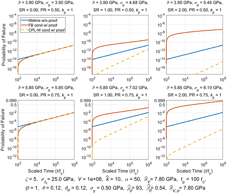
Figure 1. Tows with fibers in a planar array and with matrix parameter, φ = 1.

FIGURE 2

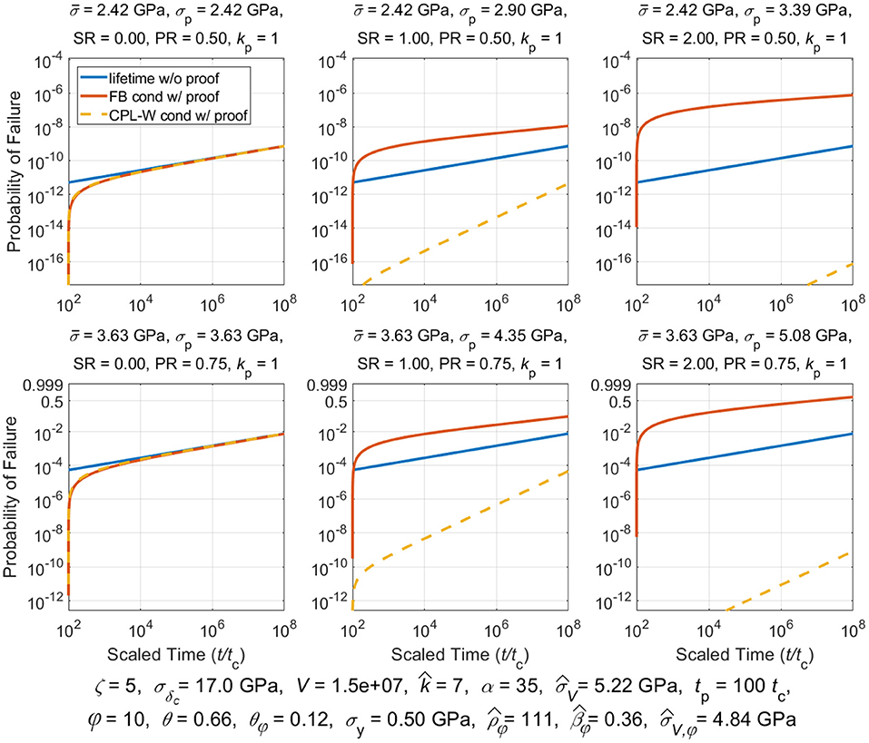
Figure 2. Tows with fibers in a planar array and matrix parameters, φ = 10 and σ_y = 0.5GPa.

FIGURE 3

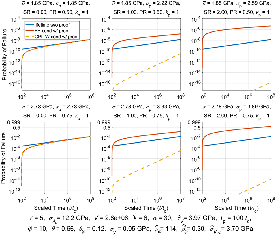
Figure 3. Tows with fibers in a planar array and matrix parameters φ = 10 and σ_y = 0.05GPa.

FIGURE 4

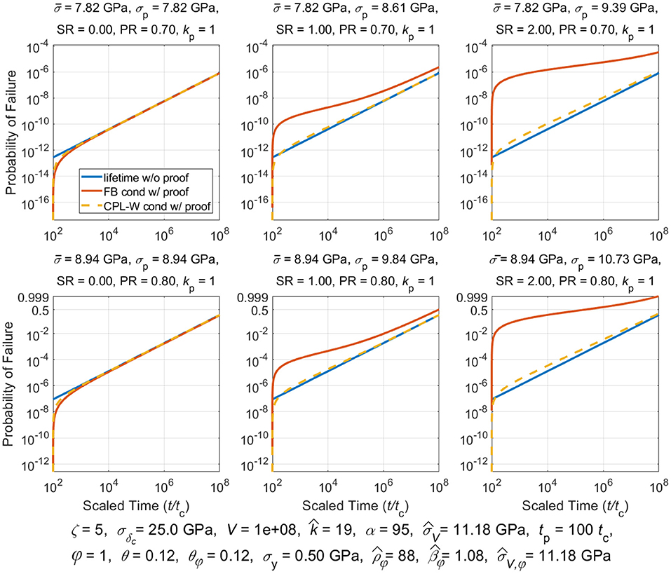
Figure 4. Tows with fibers in a hexagonal array and matrix parameter, φ = 1, and with ϕ = 2.5 and γ = 0.27 in (55) for calculating number of susceptible fibers around a cluster.

FIGURE 5

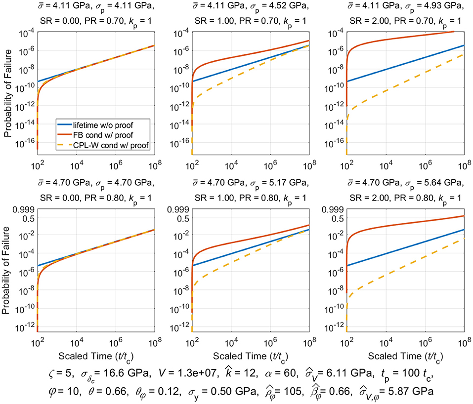
Figure 5. Tows with fibers in a hexagonal array and matrix parameters φ = 10 and σ_y = 0.50GPa, with ϕ = 2.5 and γ = 0.27 in (55) used to calculate number of susceptible fibers around a cluster.

FIGURE 6

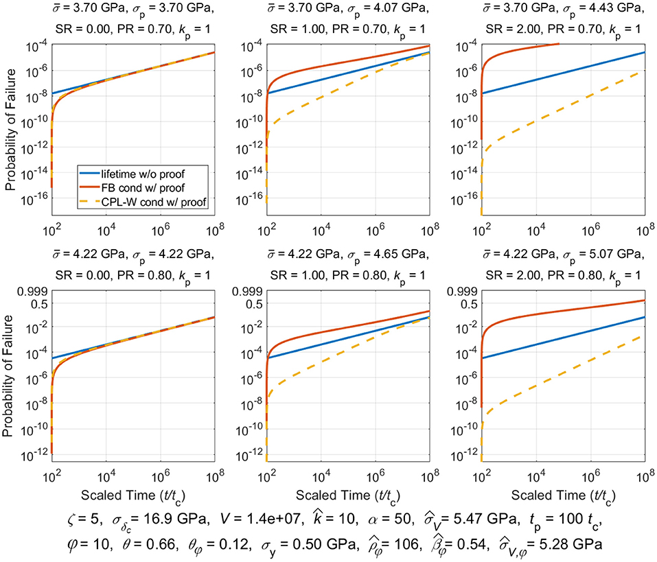
Figure 6. Tow lifetime distribution with fibers arranged in a hexagonal array with number of overloaded neighbors following (56), and with matrix parameters φ = 10 and σ_y = 0.50GPa.

Additional Parametric Details in the Application to COPVs

The second application involves predicting the strength of COPVs based on tow strength properties, as specified for the tow elements in the model, where by the Weibull shape parameter is ζ = 20, and scale parameter is ${\sigma }_{{\widehat{\delta }}_{\mathrm{\text{c}}}}=8.0\mathrm{\text{GPa}}$ corresponding to the case φ = 1, where ${\widehat{\delta }}_{\mathrm{\text{c}}}={\delta }_{\mathrm{\text{c}}}$. In Figure 7 we show results for a planar array of tows and associated load-sharing, and in Figure 8 we show results for tows in a hexagonal array and sharing load accordingly with (56) governing the number of overloaded neighbors to a cluster. In both cases we assume φ = 10 and σ_y = 0.25GPa for purposes of modeling interface creep or tow slippage in shear between tows (Results for φ = 1 are not shown).

FIGURE 7

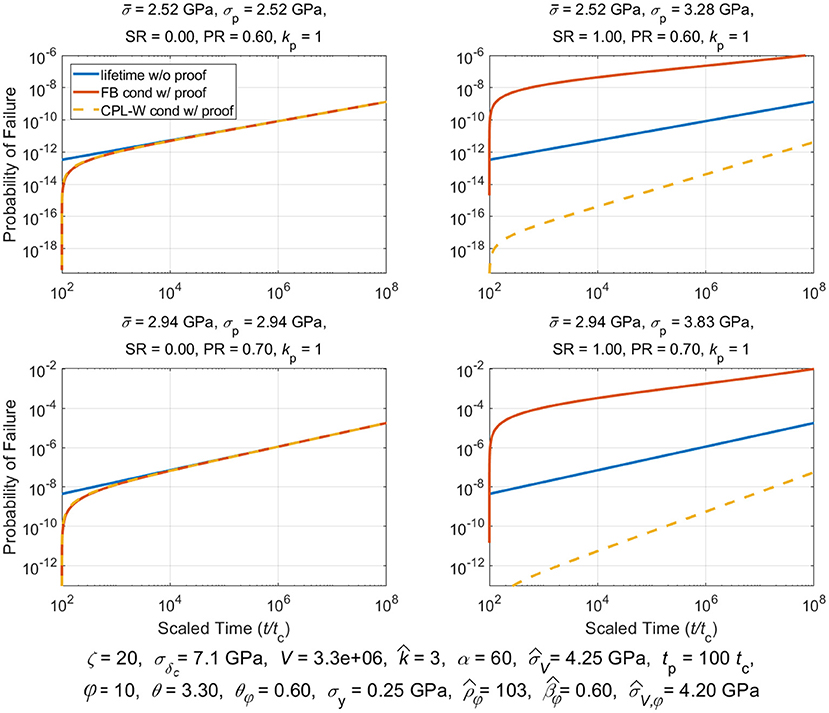
Figure 7. COPV lifetime distribution where tows are modeled as being arranged in a planar array, and with matrix parameter φ = 10 and σ_y = 0.25GPa.

FIGURE 8

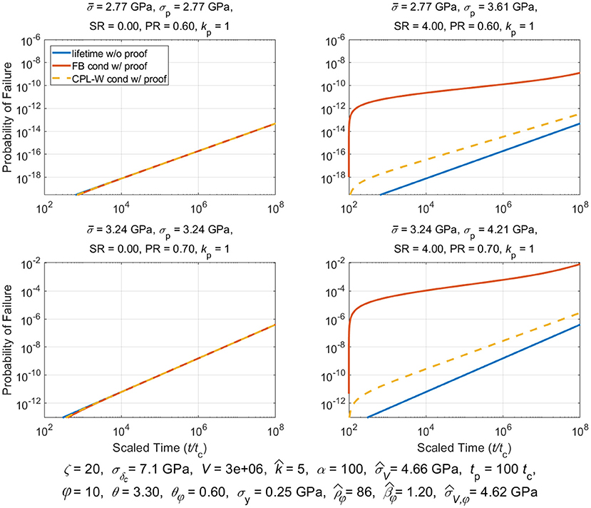
Figure 8. COPV where tows are modeled as being arranged in a hexagonal array under (56) for the number of overloaded tows around a cluster, and where φ = 10 and σ_y = 0.25GPa.

Plotted Quantities and Applied Loadings Used in Each Particular Application and Case

For all cases plotted in Figure 1 through Figure 8, time begins at t = 0, though the horizontal axes and plotting of the graphs begins only at t = t_p. For this reason, a virgin specimen initially loaded at t = 0 can potentially fail before time t_p, which is why the failure probability at time, t = t_p is already distinctly non-zero. On the other hand, a proof-tested vessel sees its proof test applied over the time period, 0 ≤ t < t_p, and if it fails it is replaced by one that has survived the proof test, at which point time continues onward, i.e. t_p ≤ t. Consequently, exactly at time t = t_p the probability of failure of the proof-tested vessel, being a conditional probability of failure, is by definition zero. However, because of the proof test it will have many broken fiber elements that otherwise would not have occurred, had it been a virgin specimen that survived to time t = t_p. Thus, only a short time later at some time, [[Mathtype-mtef1-eqn-619.mtf]], its probability of failure shoots up beyond what occurs without the proof test. This “overshoot” after the proof test is a key feature of the model that generally does not occur for the classic CPL-W model or other models.

These effects are seen in all the figures, where the solid blue line represents the failure probability vs. time for a lifetime test under a constant loading (2), i.e., absent a proof test, both for the classic power-law (CPL-W) model and the current stochastic fiber breakage (SFB) model (which happen to be the same when parameter values in (73) and (41) are appropriately matched). In cases involving a proof test under loading (3), the conditional probability of failure vs. time following survival of the proof test is given as a solid orange line for the SFB model, and a dashed yellow line for the CPL-W model. Above each figure panel is the loading condition for that particular case, where the results presented for specific tow cases are in Figures 1–6, and specific COPV cases in Figures 7, 8. The loading parameter “SR” in the various cases refers to the stress ratio used for that figure panel, which is the constant applied stress, $\bar{\sigma }$, in the lifetime test, divided by the Weibull stress scale parameter, ${\widehat{\sigma }}_{V,\phi }$, for that case. The parameter “PR” refers to the proof stress ratio used in a particular case of a figure, being the ratio of the proof stress to the applied stress in the lifetime test, ${\sigma }_{\mathrm{\text{p}}}/\bar{\sigma }$. Note that each figure presents plots for two different stress ratios and three different proof ratios in tows and two different proof ratios in COPVs. Also k_p refers to the special proof cluster size defined by (57).

Common Features of Plots Associated With a Proof Test, Whether for Tows or for COPVs

All figures show that when the stress in a proof test is the same as the lifetime stress level, i.e., ${\sigma }_{\mathrm{\text{p}}}=\bar{\sigma }$, the SFB and CPL-W models predict the same results for probability of failure vs. time, although with failure probabilities that are initially lower than when no proof test is applied. However, when ${\sigma }_{\mathrm{\text{p}}}>\bar{\sigma }$, the SFB model always predicts an higher probability of failure compared to a standard lifetime test without a proof test, which is sometimes higher by several orders of magnitude. In contrast, the CPL-W model predicts a lower probability of failure after a proof test in the typical case where 0 < β_φ < 1, and typically by several orders of magnitude. However, in the CPL-W model a higher probability of failure does occur when β_φ > 1 (see Figures 4, 8), though not of the magnitude seen in the SFP model. This is a critical difference between the two models, SFB vs CPL-W, also discussed extensively in [78] for the special case φ = 1.

Additional Features of Effects of φ and σ_y on the Strength Distribution of Tows

Figure 1 through Figure 3 show the lifetime distribution of a carbon/epoxy tow assuming a planar fiber configuration and planar load-sharing. Figures 1, 2 showing the effects of changing φ from 1 to 10 when σ_y = 0.5GPa, and Figures 2, 3 demonstrate the effect of further lowering σ_y by an order of magnitude to σ_y = 0.05GPa, while maintaining φ = 10 (when φ = 1 there is no effect from changing σ_y). In Figures 2, 3, choosing φ > 1 with ${\sigma }_{\mathrm{\text{y}}}<{\widehat{\sigma }}_V$, requires reducing, V, the number of fiber elements in the model, in order to maintain the same total material volume. This reduction in V is associated with the previously mentioned, increase in δ_c, which results in a decrease in σ_δc as well as a decrease in the critical cluster size $\widehat{k}$ from the value $\widehat{k}=10$ in Figure 1, to $\widehat{k}=7$ in Figure 2 and to $\widehat{k}=6$ in Figure 3. This reduction in $\widehat{k}$ causes a proportional lowering of the Weibull shape parameter for strength, $\widehat{\alpha }=\widehat{k}\zeta$ in (19) from $\widehat{\alpha }=50$ in Figure 1 down to $\widehat{\alpha }=30$ in Figure 3, which happens to be a more realistic value for tows compared to those obtained experimentally, but still somewhat larger. This decrease in $\widehat{\alpha }$ reflects an increase in the variability in tow strength.

A significant decrease also occurs in the Weibull scale parameter for tow strength, ${\widehat{\sigma }}_V$, from ${\widehat{\sigma }}_V=7.80\mathrm{\text{GPa}}$ in Figure 1 to ${\widehat{\sigma }}_V=5.22\mathrm{\text{GPa}}$in Figure 2 and then to ${\widehat{\sigma }}_V=3.97\mathrm{\text{GPa}}$ in Figure 3 (Effects on ${\widehat{\sigma }}_{V,\phi }$ will be discussed later in connection with lifetime behavior). This amounts to decreases of as much as 50% in strength. Once again, the Weibull shape and scale parameter values for tow strength associated with Figure 1 are overly optimistic compared to the more realistic values in Figures 2, 3. Clearly non-linear matrix creep and yielding can result in large effect in terms of lowering the composite strength and increasing its variability compared to the case of φ = 1.

Figure 4 through Figure 6 provide results similar to those in Figure 1 through Figure 3, but for the case of hexagonal fiber packing and associated load-sharing. Figures 4, 5 involve using the parameter values ϕ = 2.5 and γ = 0.27 in (55), which determines the number of fibers around a cluster susceptible to failure in growing a cluster. Figure 6 is similar to Figure 5, except that now $\varphi =\sqrt{4\pi }$ and γ = 0.5, as was used in (56), for determining the number of susceptible neighbors. Otherwise we maintain φ = 10 and σ_y = 0.5GPa. Reductions are again needed in the number of fiber elements, V, with increasing δ_c, to maintain the same overall material volume, and the result is a large decrease in the critical cluster size $\widehat{k}$ from $\widehat{k}=19$ in Figure 4 to $\widehat{k}=12$ in Figure 5 and to $\widehat{k}=10$ in Figure 6. Likewise a proportional lowering of the Weibull strength shape parameter, $\widehat{\alpha }=\widehat{k}\zeta$, occurs from $\widehat{\alpha }=95$ in Figure 4 down to $\widehat{\alpha }=50$ in Figure 6 as well as a large drop in the Weibull strength scale parameter from ${\widehat{\sigma }}_V=11.18\mathrm{\text{GPa}}$ in Figure 4 to ${\widehat{\sigma }}_V=5.47\mathrm{\text{GPa}}$ in Figure 6, which is a reduction by one-half.

Once again, the values seen in Figure 4 for φ = 1 are overly optimistic compared to the more realistic values in Figures 5, 6, as found in experiments, though still larger. Once again non-linear matrix creep and yielding can result in a large decrease in the strength of the composite and an increase in its variability.

Additional Features of Effects of φ and σ_y on the Lifetime Distribution of Tows

Figure 1 through Figure 6 demonstrate the effects on the composite tow lifetime distribution not only from changes in φ and σ_y, but also from changes in the load-sharing arrangement of the fibers in the tow (planar vs. hexagonal in two versions). The latter changes are seen in comparing the two groups of figures, namely Figure 1 through Figure 3 with Figure 4 through Figure 6.

In Figure 1 through Figure 3, a major effect of the decrease seen in $\widehat{k}$ from $\widehat{k}=10$ in Figure 1 down to $\widehat{k}=6$ in Figure 3, is to decrease the Weibull lifetime shape parameter, from ${\widehat{\beta }}_{\phi }=0.54$ to ${\widehat{\beta }}_{\phi }=0.30$. Likewise the lifetime stress scale, ${\widehat{\sigma }}_{V,\phi }$, decreases from ${\widehat{\sigma }}_{V,\phi }={\widehat{\sigma }}_V=7.80\mathrm{\text{GPa}}$ down to ${\widehat{\sigma }}_{V,\phi }=3.70\mathrm{\text{GPa}}$, a reduction by more than a factor of two. On the other hand the effect on ${\widehat{\rho }}_{\phi }$ is modest and its value increases from ${\widehat{\rho }}_{\phi }=93$ in Figure 1 to ${\widehat{\rho }}_{\phi }=114$ in Figure 3. This is caused largely by the dependence of ${\widehat{\rho }}_{\phi }$ on $\widehat{k}$ in (43). Otherwise, the plots in Figure 1 through Figure 3 show very similar behavior, with much of the difference in plotted probability values caused by the decrease in ${\widehat{\beta }}_{\phi }$ (and resulting increase in variability) thus increasing the failure probabilities since the effect of ${\widehat{\sigma }}_{V,\phi }$ is scaled out, and the change in ${\widehat{\rho }}_{\phi }$ is comparatively smaller.

Similarly in Figure 4 through Figure 6, a major effect of the decrease in $\widehat{k}$ from $\widehat{k}=19$ in Figure 4 down to $\widehat{k}=10$ in Figure 6, is to decrease the Weibull shape parameter for lifetime from ${\widehat{\beta }}_{\phi }=1.08$ in Figure 4 to ${\widehat{\beta }}_{\phi }=0.54$ in Figure 6. Note that since ${\widehat{\beta }}_{\phi }=1.08>1$, which means $\tilde{\beta }=1.08>1$ in the CPL-W model, a proof test in that model results in a slight increase in the probability of failure over time compared to having no proof test. Likewise the decrease in $\widehat{k}$ also results in a large decrease in the Weibull lifetime stress scale, ${\widehat{\sigma }}_{V,\phi }$, decreases from ${\widehat{\sigma }}_{V,\phi }={\widehat{\sigma }}_V=11.18\mathrm{\text{GPa}}$ down to the more realistic value, ${\widehat{\sigma }}_{V,\phi }=5.28\mathrm{\text{GPa}}$, again by almost a factor of two. Both parameters exhibit reductions by a factor of two. On the other hand, the effect on ${\widehat{\rho }}_{\phi }$ is a more modest increase from ${\widehat{\rho }}_{\phi }=88$ in Figure 4 to ${\widehat{\rho }}_{\phi }=106$ in Figure 6, as a result of the dependence of ${\widehat{\rho }}_{\phi }$ on $\widehat{k}$ in (43).

Otherwise, the plots in Figure 1 through Figure 6 show very similar behavior where much of the difference in plotted probability values is caused by the decrease in ${\widehat{\beta }}_{\phi }$ since the large effect of ${\widehat{\sigma }}_{V,\phi }$ is scaled out, and the change in ${\widehat{\rho }}_{\phi }$ is modest by comparison. Generally, the effects seen in Figure 1 through Figure 6 follow patterns previously discussed in [78].

Effects of φ and σ_y on COPV Strength Based on Tow Elements Having Weibull Strength

Figures 7, 8 show results for COPV strength and lifetime assuming tow elements have Weibull strength with shape parameter ζ = 20 (a more conservative value than the theoretical values in Figures 3, 6) and scale parameter that in both cases turns out to be σ_δc = 7.1GPa. Both figures assume φ = 10 and σ_y = 0.25GPa for the interface between tows, and thus, the value of σ_δc is lower than ${\sigma }_{{\widehat{\delta }}_{\mathrm{\text{c}}}}=8.0\mathrm{\text{GPa}}$ for the case φ = 1 as a result of a factor of about 10 increase in tow element length δ_c as compared to ${\widehat{\delta }}_{\mathrm{\text{c}}}$. This element length change also results in a factor of 10 reduction in V. Note that the results in Figure 7 assume planar load-sharing among tows, whereas Figure 8 assumes tows arranged and sharing load in a hexagonal configuration with (56) governing the number of overloaded tow elements surrounding a cluster of tow breaks.

The change in tow load-sharing mechanism leads to an increase in the critical cluster size, $\widehat{k}$, from $\widehat{k}=3$ in Figure 7, to $\widehat{k}=5$ in Figure 8. This in turn causes a proportional increase in the Weibull shape parameter for strength, $\widehat{\alpha }=\widehat{k}\zeta$ in (19) from $\widehat{\alpha }=60$ in Figure 7 to $\widehat{\alpha }=100$ in Figure 8, thus reflecting a substantial decrease in the variability in COPV strength. There is also a significant increase in the Weibull strength scale parameter, ${\widehat{\sigma }}_V$, from ${\widehat{\sigma }}_V=4.25\mathrm{\text{ GPa}}$ in Figure 7 to ${\widehat{\sigma }}_V=4.66\mathrm{\text{GPa}}$ in Figure 8. This increase in ${\widehat{\sigma }}_V$ of about 10% for a COPV is much less than in the case of tows, largely because the starting value of ζ is a larger value, 20, rather than 5, and the effect on the value of $\widehat{k}$ is also much smaller. Nevertheless, changing the value of φ from φ = 1 to φ = 10 together with the choice of ${\sigma }_{\mathrm{\text{y}}}=0.10\mathrm{\text{GPa}}\ll {\widehat{\sigma }}_V$ does have the effect of decreasing the COPV strength and increasing its variability (results for φ = 1 not shown).

Effects of φ and σ_y on the Lifetime Distribution of COPVs in Stress-Rupture

Figures 7, 8 also demonstrate the effects on the composite lifetime distribution of changes in the tow load-sharing arrangement from a planar array to a hexagonal array. A major effect is again to increase $\widehat{k}$ from $\widehat{k}=3$ in Figure 7 to $\widehat{k}=5$ in Figure 8, which leads to an increase the Weibull shape parameter for lifetime, from ${\widehat{\beta }}_{\phi }=0.60$ to ${\widehat{\beta }}_{\phi }=1.20$. Likewise the Weibull lifetime stress scale, ${\widehat{\sigma }}_{V,\phi }$, increases from ${\widehat{\sigma }}_{V,\phi }=4.20\mathrm{\text{GPa}}$ to ${\widehat{\sigma }}_{V,\phi }=4.62\mathrm{\text{GPa}}$. On the other hand there is a decrease in ${\widehat{\rho }}_{\phi }$, from ${\widehat{\rho }}_{\phi }=103$ to ${\widehat{\rho }}_{\phi }=86$, which in part also contributed to the large increase in ${\widehat{\beta }}_{\phi }$. Otherwise, the plots show very similar behavior, with much of the difference in plotted probability values caused by the increase in ${\widehat{\beta }}_{\phi }$ since the effect of ${\widehat{\sigma }}_{V,\phi }$ is scaled out, and there a relatively smaller change in ${\widehat{\rho }}_{\phi }$. Again since ${\widehat{\beta }}_{\phi }=1.20>1$, and thus $\tilde{\beta }=1.20>1$ in the CPLW model, a proof test in that model results in a substantial increase in the probability of failure over time compared to having no proof test. Once again, however, the increase is modest compared to the large increase seen in the SFB model of the current work.

Conclusions

In this work we have generalized the SFB model derived in [78], by extending the linearly viscoelastic matrix creep behavior into the non-linear range. The linear viscoelastic version can be obtained from the current model by setting φ = 1. Since the general form of the SFB model does not change by adding non-linear viscoelasticity, the conclusions regarding the detrimental effects of proof testing still hold as were demonstrated in Figure 1 through Figure 8.

A key advantage of the current non-linear creep model over the linear viscoelastic model with instantaneous shear modulus, G_e, is that all the above factors can be accounted for directly in the model when calculating the distribution for lifetime. This eliminates the need, in the linear model, to artificially account for fiber-matrix debonding or matrix shear failure and its effect on increasing the value δ_c when trying to make strength predictions using (17) or lifetime predictions using (41) together with (48) through (51). This is the critically important aspect of the new work.

Finally, the development of a stress-rupture model is certainly an important aspect of the overall technological challenge of designing and manufacturing highly reliable and human-safe composite structures, such as COPVS. However, such efforts still rely on the generation of experimental data, as well as drawing on databases of previous experimental work and the modeling approaches used to design the experiments and interpret the data. A comparison of various models that have been used (which are largely phenomenological such as the CPL-W model), is given in [1]. General and parametric features of experimental data for unidirectional composites that consist of a wide variety of fibers in a polymer matrix, as well as commonly used statistical methods (such as maximum likelihood) are discussed in [2]. Also, in [2] uncertainty distributions on model parameters are obtained using Monte Carlo simulation. In [3] a unified maximum-likelihood method is developed for the CPL-W model with the goal of reducing uncertainty in parameter and reliability estimation. Finally, in [4] further maximum likelihood analysis is devoted to removing bias and characterizing uncertainty in both model parameters and reliability estimates. Monte Carlo simulation is used to study uncertainty in the parameter and reliability estimates and to assess bias. In both [3] and [4] the method is demonstrated using strength and lifetime data generated on small carbon/epoxy COPVs tested at the NASA White Sands Test Facility over a two and a half year period.

Data Availability Statement

The original contributions presented in the study are included in the article/Supplementary Material, further inquiries can be directed to the corresponding author/s.

Author Contributions

All authors listed have made a substantial, direct and intellectual contribution to the work, and approved it for publication.

Funding

Funding for this work was provided under National Institute of Standards and Technology (NIST) agreement ID 70NANB14H323 for Stuart Leigh Phoenix and National Institute of Standards and Technology (NIST) agreement ID 70NANB18H222 for AE-W.

Conflict of Interest

The authors declare that the research was conducted in the absence of any commercial or financial relationships that could be construed as a potential conflict of interest.

Supplementary Material

The Supplementary Material for this article can be found online at: https://www.frontiersin.org/articles/10.3389/fphy.2021.644815/full#supplementary-material

References

1. Engelbrecht-Wiggans AE, Phoenix SL. Comparison of probabilistic models for stress rupture failure in continuous unidirectional fiber composite structures. J Mater Sci. (2018) 53:7431–52. doi: 10.1007/s10853-018-2101-2

CrossRef Full Text | Google Scholar

2. Engelbrecht-Wiggans AE, Phoenix SL. Comparison of maximum likelihood approaches for analysis of composite stress rupture data. J Mater Sci. (2016) 51:6639–61. doi: 10.1007/s10853-016-9950-3

CrossRef Full Text | Google Scholar

3. Engelbrecht-Wiggans AE, Phoenix SL. Analysis of stress rupture data on fiber composites: Part 1- A unified maximum likelihood method. J Sp Saf Eng. (2017) 4:9–14. doi: 10.1016/j.jsse.2017.03.002

CrossRef Full Text | Google Scholar

4. Engelbrecht-Wiggans AE, Phoenix SL. Analysis of stress rupture data on fiber composites. Part 2. Determining uncertainty and removing bias in estimates. J Sp Saf Eng. (2017) 4:83–94. doi: 10.1016/j.jsse.2017.06.003

CrossRef Full Text | Google Scholar

5. Pradhan S, Hansen A, Chakrabarti BK. Failure processes in elastic fiber bundles. Rev Mod Phys. (2010) 82:499–555. doi: 10.1103/RevModPhys.82.499

CrossRef Full Text | Google Scholar

6. Alava MJ, Nukala PKVV, Zapperi S. Statistical models of fracture. Adv Phys. (2006) 55:349–476. doi: 10.1080/00018730300741518

CrossRef Full Text | Google Scholar

7. Kun F, Zapperi S, Herrmann HJ. Damage in fiber bundle models. Eur Phys J B. (2000) 17:269–79. doi: 10.1007/PL00011084

CrossRef Full Text | Google Scholar

8. Roy S, Biswas S, Ray P. Modes of failure in disordered solids. Phys Rev E. (2017) 96:063003. doi: 10.1103/PhysRevE.96.063003

CrossRef Full Text | Google Scholar

9. Phoenix SL, Beyerlein IJ. Statistical strength theory for fibrous composite materials. Compreh Comp Mater. (2000) 1:559–639. doi: 10.1016/B0-08-042993-9/00056-5

CrossRef Full Text | Google Scholar

10. Mahesh S, Phoenix SL, Beyerelin IJ. Strength distributions and size effects for 2D and 3D composites with Weibull fibers in an elastic matrix. Int J Fract. (2002) 115:41–85. doi: 10.1023/A:1015729607223

CrossRef Full Text | Google Scholar

11. Alava MJ, Nukala PKVV, Zapperi S. Size effects in statistical fracture. J Phys D Appl Phys. (2009) 42:214012. doi: 10.1088/0022-3727/42/21/214012

CrossRef Full Text | Google Scholar

12. Bazant ZP, Le J-L, Bazant M. Scaling of strength and lifetime probability distributions of quasibrittle structures based on atomistic fracture mechanics. PNAS. (2009) 106:11484–9. doi: 10.1073/pnas.0904797106

PubMed Abstract | CrossRef Full Text | Google Scholar

13. Phoenix SL, Ibnabdeljalil M, Hui C-Y. Size effects in the distribution for strength of brittle matrix fibrous composites. Int J Solids Struct. (1997) 34:545–68. doi: 10.1016/S0020-7683(96)00034-0

CrossRef Full Text | Google Scholar

14. Roux S. Thermally activated breakdown in the fiber-bundle model. Phys Rev E. (2000) 62:6164–9. doi: 10.1103/PhysRevE.62.6164

PubMed Abstract | CrossRef Full Text | Google Scholar

15. Yewande OE, Moreno Y, Kun F, Hidalgo RC, Herrmann HJ. Time evolution of damage under variable ranges of load transfer. Phys Rev E. (2003) 68:026116. doi: 10.1103/PhysRevE.68.026116

PubMed Abstract | CrossRef Full Text | Google Scholar

16. Roy S, Biswas S, Ray P. Failure time in heterogeneous systems. Phys Rev Res. (2019) 1:033047. doi: 10.1103/PhysRevResearch.1.033047

CrossRef Full Text | Google Scholar

17. Clemente MA, Gómez JB, Pacheco AF. Time to failure of dynamic local load-sharing fiber bundle models in 1 to 3 dimensions. Physica D. (2019) 390:1–8. doi: 10.1016/j.physd.2018.10.003

CrossRef Full Text | Google Scholar

18. Coleman BD. Time dependence of mechanical breakdown phenomena. J Appl Phys. (1956) 27:862–66. doi: 10.1063/1.1722504

CrossRef Full Text | Google Scholar

19. Coleman BD. A stochastic process model for mechanical breakdown. Trans Soc Rheol. (1957) 1:153–68. doi: 10.1122/1.548812

CrossRef Full Text | Google Scholar

20. Coleman BD. Time dependence of mechanical breakdown in bundles of fibers. I. Constant total load. J Appl Phys. (1957) 28:1058–64. doi: 10.1063/1.1722907

CrossRef Full Text | Google Scholar

21. Coleman BD. Time dependence of mechanical breakdown in bundles of fibers. III. The power- law breakdown rule. Trans Soc Rheol. (1958) 2:195–218. doi: 10.1122/1.548830

CrossRef Full Text | Google Scholar

22. Tobolsky A, Eyring H. Mechanical properties of polymeric materials. J Chem Phys. (1943) 11:125–34. doi: 10.1063/1.1723812

CrossRef Full Text | Google Scholar

23. Phoenix SL. The asymptotic distribution for the time to failure of a fibre bundle. Adv Appl Probab. (1979) 11:153–87. doi: 10.1017/S0001867800031748

CrossRef Full Text | Google Scholar

24. Newman WI, Phoenix SL. Time-dependent fiber bundles with local load sharing. Phys Rev E. (2001) 63:021507. doi: 10.1103/PhysRevE.63.021507

PubMed Abstract | CrossRef Full Text | Google Scholar

25. Phoenix SL, Newman WI. Time-dependent fiber bundles with local load sharing. II. General Weibull fibers. Phys Rev E. (2009) 80:066115. doi: 10.1103/PhysRevE.80.066115

PubMed Abstract | CrossRef Full Text | Google Scholar

26. Mattsson A, Uesaka T. Time-dependent statistical failure of fiber networks. Phys Rev E. (2015) 92:042158. doi: 10.1103/PhysRevE.92.042158

PubMed Abstract | CrossRef Full Text | Google Scholar

27. Mattsson A, Uesaka T. Time-dependent breakdown of fiber networks: uncertainty of lifetime. Phys Rev E. (2017) 95:053005. doi: 10.1103/PhysRevE.95.053005

PubMed Abstract | CrossRef Full Text | Google Scholar

28. Halasz Z, Danku Z, Kun F. Competition of strength and stress disorder in creep rupture. Phys Rev E. (2012) 85:016116. doi: 10.1103/PhysRevE.85.016116

PubMed Abstract | CrossRef Full Text | Google Scholar

29. Ibnabdeljalil M, Phoenix SL. Creep rupture of brittle matrix composites reinforced with time dependent fibers: Scalings and Monte Carlo simulations. J Mech Phys Solids. (1995) 43:897–931. doi: 10.1016/0022-5096(95)00008-7

CrossRef Full Text | Google Scholar

30. Kelly A, McCartney LN. Failure by stress corrosion of bundles of fibres. Proc R Soc London A Math Phys Sci. (1981) 374:475–89. doi: 10.1098/rspa.1981.0032

CrossRef Full Text | Google Scholar

31. Iyengar N, Curtin WA. Time dependent failure in fiber-reinforced composites by fiber degradation. Acta Mater. (1997) 45:1489–502. doi: 10.1016/S1359-6454(96)00260-1

CrossRef Full Text | Google Scholar

32. Goda K. Creep-rupture lifetime simulation of unidirectional metal matrix composites with andwithout time-dependent fiber breakage. Int J Plasticity. (2002) 18:1729–48. doi: 10.1016/S0749-6419(01)00038-9

CrossRef Full Text | Google Scholar

33. Yoshioka N, Kun F, Ito N. Kinetic Monte Carlo algorithm for thermally induced breakdown of fiber bundles. Phys Rev E. (2015) 91:033305. doi: 10.1103/PhysRevE.91.033305

PubMed Abstract | CrossRef Full Text | Google Scholar

34. Linga G, Ballone P, Hansen A. Creep rupture of fiber bundles: A molecular dynamics investigation. Phys Rev E. (2015) 92:022405. doi: 10.1103/PhysRevE.92.022405

PubMed Abstract | CrossRef Full Text | Google Scholar

35. Kun F, Hidalgo RC, Herrmann HJ, Pal KF. Scaling laws of creep rupture of fiber bundles. Phys Rev E. (2003) 67:061802. doi: 10.1103/PhysRevE.67.061802

PubMed Abstract | CrossRef Full Text | Google Scholar

36. Kovacs K, Nagy S, Hidalgo RC, Kun F, Herrmann HJ, Pagonabarraga I. Critcal rupture in a bundle of slowly relaxing fibers. Phys Rev E. (2008) 77:036102 doi: 10.1103/PhysRevE.77.036102

PubMed Abstract | CrossRef Full Text | Google Scholar

37. Hidalgo RC, Kun F, Herrmann HJ. Slow relaxation of fiber composites, variable range of interaction approach. Physica A. (2005) 347:402–410. doi: 10.1016/j.physa.2004.08.039

CrossRef Full Text | Google Scholar

38. Lifshitz JM, Rotem A. Time-dependent longitudinal strength of unidirectional fiber composites. Fibre Sci Technol. (1970) 3:1–19. doi: 10.1016/0015-0568(70)90023-0

CrossRef Full Text | Google Scholar

39. Iyengar N, Curtin WA. Time dependent failure in fiber-reinforced composites by matrix and interface shear creep. Acta Mater. (1997) 45:3419–29. doi: 10.1016/S1359-6454(96)00412-0

CrossRef Full Text | Google Scholar

40. Ohno N, Miyake T. Stress relaxation in broken fibers in unidirectional composites: modeling and application to creep rupture analysis. Int J Plasticity. (1999) 15:167–89. doi: 10.1016/S0749-6419(98)00063-1

CrossRef Full Text | Google Scholar

41. Koyanagi J, Hatta H, Ogawa F, Kawada H. Time-dependent reduction of tensile strength caused by interfacial degradation under constant strain duration in UD-CFRP. J Compos Mater. (2007) 41:3007–26. doi: 10.1177/0021998307082175

CrossRef Full Text | Google Scholar

42. Phoenix SL, Schwartz P, Robinson HH. Statistics for the strength and lifetime in creep-rupture of model carbon/epoxy composites. Compos Sci Technol. (1988) 32:81–120. doi: 10.1016/0266-3538(88)90001-2

CrossRef Full Text | Google Scholar

43. Otani H, Phoenix SL, Petrina P. Matrix effects on lifetime statistics for carbon fiber-epoxy microcomposites in creep-rupture. J Mater Sci. (1988) 26:1955–1970. doi: 10.1007/BF00543630

CrossRef Full Text | Google Scholar

44. Mahesh S, Phoenix SL. Lifetime distributions for unidirectional fibrous composites under creep-rupture loading. Int J Fract. (2004) 127:303–60. doi: 10.1023/B:FRAC.0000037675.72446.7c

CrossRef Full Text | Google Scholar

45. Nakada M, Miyano Y, Morisawa Y, Nishida H, Hayashi Y, Uzawa, et al. Prediction of statistical life time for unidirectional CFRTP under creep loading. J Reinforced Plastics and Composites. (2019) 38:938–46. doi: 10.1177/0731684419854213

CrossRef Full Text | Google Scholar

46. Miyano Y, Nakada M. Accelerated testing methodology for durability of CFRP. Composites Part B. (2020) 191:107977 doi: 10.1016/j.compositesb.2020.107977

CrossRef Full Text | Google Scholar

47. Blassiau S, Thionnet A, Bunsell AR. Micromechanisms of load transfer in a unidirectional carbon fibre–reinforced epoxy composite due to fibre failures. Part. 1: Micromechanisms and 3D analysis of load transfer: The elastic case. Compos Struct. (2006) 74:303–18. doi: 10.1016/j.compstruct.2005.04.013

CrossRef Full Text | Google Scholar

48. Blassiau S, Thionnet A, Bunsell AR. Micromechanisms of load transfer in a unidirectional carbon fibre–reinforced epoxy composite due to fibre failures. Part. 2: Influence of viscoelastic and plastic matrices on the mechanisms of load transfer. Compos Struct. (2006) 74:319–31. doi: 10.1016/j.compstruct.2005.04.029

CrossRef Full Text | Google Scholar

49. Blassiau S, Thionnet A, Bunsell AR. Micromechanisms of load transfer in a unidirectional carbon fibre-reinforced epoxy composite due to fibre failures: Part 3. Multiscale reconstruction of composite behaviour. Compos Struct. (2008) 82:312–23 doi: 10.1016/j.compstruct.2007.05.004

CrossRef Full Text | Google Scholar

50. Bunsell AR, Thionnet A. Life prediction for carbon fibre filament wound composite structures. Philosophical Magazine. (2010) 90:4129–46. doi: 10.1080/14786430903575140

CrossRef Full Text | Google Scholar

51. Thionnet A, Chou H-Y, Bunsell A. Fibre break failure processes in unidirectional composites. Part. 1: Failure and critical damage state induced by increasing tensile loading. Appl Compos Mater. (2015). 22:119–40. doi: 10.1007/s10443-014-9397-0

CrossRef Full Text | Google Scholar

52. Thionnet A, Chou H-Y, Bunsell A. Fibre break failure processes in unidirectional composites. Part. 2: Failure and critical damage state induced by sustained tensile loading. Appl Compos Mater. (2015). 22:141–55. doi: 10.1007/s10443-014-9398-z

CrossRef Full Text | Google Scholar

53. Thionnet A, Chou H-Y, Bunsell A. Fibre break failure processes in unidirectional composites. Part. 3: Unidirectional plies included in laminates. Appl Compos Mater. (2015). 22:157–69. doi: 10.1007/s10443-014-9399-y

CrossRef Full Text | Google Scholar

54. Thionnet A, Bunsell AR. Fibre break failure processes in unidirectional composites: evaluation of critical damage states. Phil Trans R Soc A. (2015) 374:20150270. doi: 10.1098/rsta.2015.0270

PubMed Abstract | CrossRef Full Text | Google Scholar

55. Thionnet A, Bunsell A, Chou H-Y. Intrinsic mechanisms limiting the use of carbon fiber composite pressure vessels. ASME J Press Vessel Technol. (2016) 138:060910. doi: 10.1115/1.4032914

CrossRef Full Text | Google Scholar

56. Farquhar DS, Mutrelle FM, Phoenix SL, Smith RL. Lifetime statistics for single graphite fibers in creep rupture. J Mater Sci. (1989) 24:2131–64. doi: 10.1007/BF02385436

CrossRef Full Text | Google Scholar

57. Miyake T, Yamakawa N, Ohno N. Measurement of stress relaxation in broken fibers embedded in epoxy using Raman spectroscopy. J Mater Sci. (1998) 33:5177–83. doi: 10.1023/A:1004427819540

CrossRef Full Text | Google Scholar

58. Holmes GA, Peterson RC, Hunston DL, McDonough WG, Schutte CL. The effect of non-linear viscoelasticity on interfacial shear strength measurements. In: Schapery RA, Sun CT, editors. Time Dependent and Non-linear Effects in Polymers and Composites, ASTM STP1357. West Conshohocken, PA: American Society for Testing and Materials. p. 98–117. doi: 10.1520/STP15831S

CrossRef Full Text | Google Scholar

59. Beyerlein IJ, Zhou CH, Schadler LS. A time dependent micro-mechanical fiber composite model for inelastic zone growth in viscoelastic matrices. Int J Sol Struct. (2000) 40:2171–94. doi: 10.1016/S0020-7683(03)00021-0

CrossRef Full Text | Google Scholar

60. Zhou CH, Schadler LS, Beyerlein IJ. Time-dependent micromechanical behavior in graphite/epoxy composites under constant load: a combined experimental and theoretical study. Acta Mater. (2002) 50:365–77. doi: 10.1016/S1359-6454(01)00353-6

CrossRef Full Text | Google Scholar

61. Zhou CH, Beyerlein IJ, Schadler LS. Time-dependent micromechanical behavior in graphite/epoxy composites under constant load at elevated temperatures. J Mater Sci. (2003) 38:877–84. doi: 10.1023/A:1022348419344

CrossRef Full Text | Google Scholar

62. Zhou CH, Schadler LS, Beyerlein IJ. Stress concentrations in graphite/epoxy model composites during creep at room temperature and elevated temperatures. J Compos Mater. (2004) 38:417–33. doi: 10.1177/0021998304040551

CrossRef Full Text | Google Scholar

63. Lagoudas DC, Hui C-Y, Phoenix SL. Time evolution of overstress profiles near broken fibers in a composite with a viscoelastic matrix. Int J Solids Struct. (1989) 25:45–66. doi: 10.1016/0020-7683(89)90103-0

CrossRef Full Text | Google Scholar

64. Beyerlein IJ, Phoenix SL, Raj R. Time evolution of stress redistribution around multiple fiber breaks in a composite with viscous and viscoelastic matrices. Int J Solids Struct. (1998) 35:3177–211. doi: 10.1016/S0020-7683(98)00010-9

CrossRef Full Text | Google Scholar

65. Beyerlein IJ. Stress fields around cracks with a viscous matrix and discontinuous fiber bridging, Compos Sci. Technol. (2000) 60:2309–26. doi: 10.1016/S0266-3538(00)00027-0

CrossRef Full Text | Google Scholar

66. Mason DD, Hui C-Y, Phoenix SL. Stress profiles around a fiber break in a composite with a non-linear, power law creeping matrix. Int J Solids Struct. (1992) 29:2829–54. doi: 10.1016/0020-7683(92)90143-H

CrossRef Full Text | Google Scholar

67. Ohno N, Ando T, Miyake T, Biwa S. A variational method for unidirectional fiber-reinforced composites with matrix creep. Int J Solids Struct. (2002) 39:150–74. doi: 10.1016/S0020-7683(01)00147-0

CrossRef Full Text | Google Scholar

68. Hedgepeth JM. Stress concentrations in filamentary structures. Washington, DC: NASA. (1961).

Google Scholar

69. Hedgepeth JM, Van Dyke P, Dyke P Van. Local stress concentrations in imperfect filamentary composite materials. J Compos Mater. (1967) 1:294–309. doi: 10.1177/002199836700100305

CrossRef Full Text | Google Scholar

70. Fichter WB. Stress Concentration Around Broken Filaments in a Filament-Stiffened Sheet. Washington, DC: NASA TN D-5453. (1969).

Google Scholar

71. McCarthy ED, Kim JH, Heckert NA, Leigh SD, Gilman JW, Holmes GA. The fiber break evolution process in a 2-D epoxy/glass multi-fiber array. Compos Sci Technol. (2015) 121:73–81. doi: 10.1016/j.compscitech.2014.10.013

CrossRef Full Text | Google Scholar

72. Smith RL, Phoenix SL, Greenfield MR, Henstenburg RB, Pitt RE. Lower-tail approximations for the probability of failure of 3-D fibrous composites with hexagonal geometry. P Roy Soc Lond A. (1983) 388:353–91. doi: 10.1098/rspa.1983.0087

CrossRef Full Text | Google Scholar

73. Curtin WA. Size scaling of strength in heterogeneous materials Phys Rev Lett. (1998) 80:1445–8. doi: 10.1103/PhysRevLett.80.1445

CrossRef Full Text | Google Scholar

74. Gupta A, Mahesh S, Keralavarma SM. Strength distribution of large unidirectional composite patches with realistic load sharing. Phys Rev E. (2017) 96:043002. doi: 10.1103/PhysRevE.96.043002

PubMed Abstract | CrossRef Full Text | Google Scholar

75. Habeeb CNI, Mahesh S. Strength distribution of planar local load-sharing bundles. Phys Rev E. (2015) 92:022125. doi: 10.1103/PhysRevE.92.022125

PubMed Abstract | CrossRef Full Text | Google Scholar

76. Mahesh S, Gupta A, Kachhwah US, Sheikh N. A fast algorithm to simulate the failure of a periodic elastic fibre composite. Int J Fract. (2019) 217:127–35. doi: 10.1007/s10704-019-00374-w

CrossRef Full Text | Google Scholar

77. Yentl Swolfs S, Ignaas Verpoest I, Larissa Gorbatikh L. Issues in strength models for unidirectional fibre-reinforced composites related to Weibull distributions, fibre packings and boundary effects. Compos Sci Technol. (2015) 114:4249. doi: 10.1016/j.compscitech.2015.04.002

CrossRef Full Text | Google Scholar

78. Engelbrecht-Wiggans AE, Phoenix SL. A stochastic model based on fiber breakage and matrix creep for the stress-rupture failure of unidirectional continuous fiber composites. Int J Fract. (2019) 217:1–34. doi: 10.1007/s10704-019-00359-9

CrossRef Full Text | Google Scholar

79. Christensen RM. Interactive mechanical and chemical degradation in organic materials. Int J Solids Struct. (1984) 20:791–804. doi: 10.1016/0020-7683(84)90066-0

CrossRef Full Text | Google Scholar