Dense Networks With Mixture Degree Distribution

1 Introduction

The exploding interest in complex networks during the several decades of the 21st century is rooted in the discovery that despite the diversity of complex networks, the structure and the evolution of each network are driven by a common set of basic laws and principles. Examples include the Internet and the World Wide Web [1], biological networks [2], social networks [3], and communication networks [4, 5], to mention but a few. There are two common considerable properties, the small-world effect and the scale-free feature. The well-known WS-network (Watts and Strogatz, WS) was proposed by Watts and Strogatz in Nature to explain small-world phenomena in diverse networks by two indices, diameter and clustering coefficient [6]. The most pioneering of generally studied networks is the BA-network (Barabási and Albert, BA) built by Barabási and Albert in Science using two rules, namely, growth and preferential attachment [7].

In currently existing studies, the main concentration is to create networks which have scale-free and small-world properties as mentioned above. However, most networks are sparse, which means that the average degree of networks is asymptotically equal to a positive constant under the limitation of a large number of vertices. The principal reason is that numbers of real-world networks have been found to indicate sparsity. On the contrary, a few scholars have discovered the existence of dense networks in [8, 9]. For probing such networks, several available networks have been presented and analytically explored with primary methods, including mean-field theory [10, 11], generate function [12], and rate equation [13, 14]. In particular, the vast majority of these networks are proved to have no scale-free feature. To put this in another way, the degree distribution of these networks does not obey the power-law distribution. Therefore, it is of interest to develop new theoretical frameworks for producing networks with both the density feature and the scale-free feature. Here, we propose a class of networks with the appropriate structural properties mentioned above. Specifically speaking, these networks are precisely proved to be not only scale-free and small-world but also dense. Throughout this article, because graphs are abstract representations of networks, there is no need to distinguish between graph and network, which indicates that these two terms are considered to be the same.

The remainder of this article can be organized into the following sections. In Section 2, our task is to introduce network construction and discuss some extensively reported structural properties, including the average degree, mixture degree distribution, small-world property, and mean first-passage time. Among them, our networks are analytically proved to show both the density and scale-free features since the power-law exponent of cumulative degree distribution is equal to constant 2. Afterward, all the networks have a smaller diameter and a higher clustering coefficient, suggesting that they share the small-world property. Then, we derive an explicit expression of the mean first-passage time on our networks associated with the trapping problem. Finally, we close this article with a Conclusion and Discussions in the last section.

2 Network Construction and Topological Properties

In this section, our intention is to generate a class of networks: let $N\left(t;m\right)$ denote the network with parameter m and step $t\left(t\ge 0\right)$. Then, we investigate some topological properties of our networks under consideration, including the density feature, mixture degree distribution, small-world property, and mean first-passage time.

A Network Construction

Here, we will present our network, $N\left(t;m\right)\left(m\ge 2\right)$. The network is built in an iterative fashion, with each iteration, with respect to the elements, generated in the previous steps. We divide this process into the following steps.

Step 0: We start from a single vertex, we designate it as the active vertex of the network, and the active vertex is placed in the layer zero, denoted by $L=0$.

Step 1: We add a cycle $C_m$ with m vertices and m edges, each vertex in the cycle is labeled as 0, and we connect each vertex labeled as 0 to the active vertex; then, we obtain $N\left(1;m\right)$, all the cycle’s vertices of network $N\left(1;m\right)$ at the layer $L=1$.

Step 2: We generate m replicas of $N\left(1;m\right)$, each replica identical to the network created in the previous iteration (step 1), add a new vertex regarded as an active vertex, connect each of the bottom vertices of these m replicas to the new active vertex, and attach each of the non-bottom vertices of the m replicas to form an m cycle, so we acquire $N\left(2;m\right)$, where the bottom vertices of network $N\left(1;m\right)$ at the layer $L=2$. Figure 1 explains the process of obtaining our network $N\left(2,m\right)$.

FIGURE 1

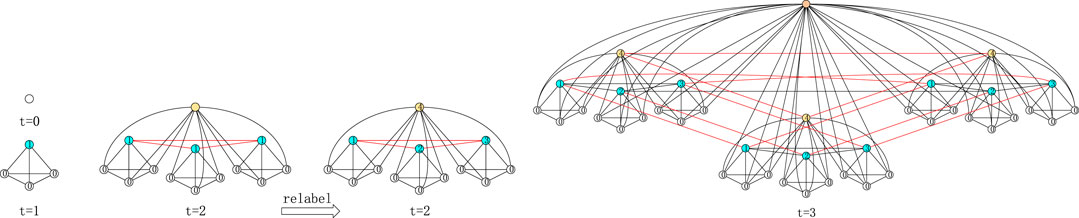
FIGURE 1. Illustration of iterative construction leads to proposed network $N\left(t;m\right)$ with $m=3$ at time $t=0,t=1,t=2,t=3$ respectively, showing the first four steps of the iterative process.

Step 3: We add m replicas of $N\left(2;m\right)$ and create a new active vertex, and then join each of the bottom vertices of these m replicas with the active vertex, and connect each of the non-bottom vertices of these m replicas to form $3^{3-1}-1/2$ cycles; thus, we get $N\left(3;m\right)$.

These steps can be easily generalized. In fact, step t will involve the following operation:

Step t: We add m replicas of $N\left(t-1;m\right)$, with each being identical to the network created in the previous iteration (step $t-1$); create a new vertex treated as an active vertex; link each of the bottom vertices of these m replicas with the active vertex; and connect each of the non-bottom vertices of these m replicas to produce $3^{t-1}-1/2$ cycles; thus, we arrive at the network $N\left(t;m\right)$.

Indefinitely repeating the steps of replication and connection, apparently, we obtain a class of networks. As an illustrative example, a network $N\left(3;3\right)$ for the particular case of $m=3$ is shown in the right of Figure 1.

Now, we compute some related basic parameters of our networks by construction. Let $V\left(t;m\right)$ and $E\left(t;m\right)$ denote the set of vertices and edges, with the number of vertices $\left|V\left(t;m\right)\right|$ and the number of edges $\left|E\left(t;m\right)\right|$ of $N\left(t;m\right)$, respectively. According to the growth steps of network $N\left(t;m\right)$, we can easily compute and get a pair of equations satisfied by the number of vertices $\left|V\left(t;m\right)\right|$ and the number of edges $\left|E\left(t;m\right)\right|$ at step t as follows:

$\{\begin{array}{l}\left|V\left(t;m\right)\right|=m\left|V\left(t-1;m\right)\right|+1\\ \left|E\left(t;m\right)\right|=m\left|E\left(t-1;m\right)\right|+\frac{m^{t+1}-m}{m-1}\end{array}.(1)$

At step $t=0$, clearly, there is $\left|V\left(0;m\right)\right|=1$ and $\left|E\left(0;m\right)\right|=0$. At step $t=1$, we have $\left|V\left(1;m\right)\right|=m+1$ and $\left|E\left(1;m\right)\right|=m\left(m+1\right)/2$. According to known conditions, we straightforwardly calculate the value of $\left|V\left(t;m\right)\right|$ and $\left|E\left(t;m\right)\right|$ from Eq. 1 and arrive at

$\{\begin{array}{l}\left|V\left(t;m\right)\right|=\frac{m^{t+1}-1}{m-1}\\ \left|E\left(t;m\right)\right|=\left|E\left(1;m\right)\right|m^{t+1}+\frac{\left(t-1\right)m^{t+1}-\frac{m^t-m}{m-1}}{m-1}\end{array}(2)$

Until now, we have finished the construction of our networks and computed certain fundamental quantities. It is an extremely evident fact to discover the hierarchy of our network related to the step. It is worth noticing that the involved network construction with hierarchy has been discussed in [1]. In [1], Ravasz et al. constructed a hierarchical network that combines the scale-free property with a high clustering. However, it should be noted that the approach adopted in this article is slightly different from the approach in [1]. While Ravasz etal. applied an iterative process for all vertices, our method is based on an idea that the next network $N\left(t;m\right)$ is created by connecting a part of vertices of each replica $N\left(t-1;m\right)$ of the proceeding model to an active vertex instead of all vertices in network $N\left(t-1;m\right)$. What calls for special attention is that for different m, our networks are different due to the number of vertices and edges being different, but the topological structure of our networks is the same. Additionally, as will be shown later, our network $N\left(t;m\right)$ are proven to have some distinguished topological properties, such as the density feature and mixture degree distribution.

B Topological Properties

As has been mentioned above, we mainly focus on the investigation of certain topological properties related to the potential structure of the proposed network. In this section, we will calculate several topological properties, including the density feature, mixture degree distribution, small-world property, and mean first-passage time. What we present here will be significant constituents in the coming subsections.

Density feature: A key topological structure of a network is its average degree. Average degree $\langle k\left(t;m\right)\rangle$ can be defined as the average value of all such vertex degrees over the entire network, which is applied to judge whether the network is sparse or dense. One can call a network sparse if $\left|E\left(t;m\right)\right|\ll \left|V\left(t;m\right)\right|\left(\left|V\left(t;m\right)\right|-1\right)/2;$ in other words, the value of $\langle k\left(t;m\right)\rangle$ tends to a finite and positive real value in the large number of vertices [15]. According to the definition of sparsity, the majority of real networks with scale-free properties, both stochastic and deterministic, are sparse. Yet, for our networks, we have

$\langle k\left(t;m\right)\rangle =\frac{2\left|E\left(t;m\right)\right|}{\left|V\left(t;m\right)\right|}\sim 2\left[t-1+\left|E\left(1;m\right)\right|\left(m-1\right)\right].(3)$

We give a detailed calculation process of the average degree in the Appendix. From Eq. 3, it goes without saying that the average degree $\langle k\left(t;m\right)\rangle$ increases linearly with t and does not tend to a real positive constant. In the large number of vertices, the average degree $\langle k\left(t;m\right)\rangle$ of Eq. 3 approaches to infinity, as shown in Figure 2. Consequently, we have the result that our network $N\left(t;m\right)$ turns out to be of density. It can be said with certainty that our networks are different from some real-world networks with sparse networks, such as hierarchical networks [1] and deterministic networks [16]. Therefore, our network $N\left(t;m\right)$ can be selected as an underlying network to reveal some remarkable properties behind those dense networks in real life.

FIGURE 2

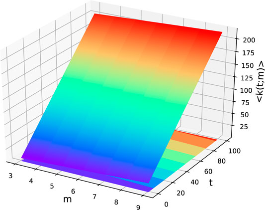
FIGURE 2. Diagram of the average degree $\langle k\left(t;m\right)\rangle$ of network $N\left(t;m\right)$.

Mixture degree distribution: The concept of degree is the most fundamental character and measure of a vertex in a network. Since in a network every vertex has a degree value, some large and some small, the distribution of vertex in the network is a key topological feature, which may be of great concern in application. The degree distribution is one of the most important topological features of a network. Degree distribution can be applied to determine whether a given network is scalefree or not. Combined with the process of network construction, it is straightforward to find that the degree spectrum of network $N\left(t;m\right)$ is a series of discrete real values. Armed with the above constructions and the method proposed by Dorogovtsev, the cumulative degree distribution of our networks can be calculated in a discrete form, as follows in [17]:

$P_{cum}\left(k\ge k_i\right)=\frac{{\displaystyle {\sum }_{k\ge k_i}{N}_k}}{\left|V\left(t;m\right)\right|},(4)$

where notation $N_k$ denotes the total number of vertices with a degree exactly equal to k in network $N\left(t;m\right)$. As stated in Eq. 4, according to the vertex degree of our networks, we need to classify all the vertices of networks to determine the degree distribution of our networks.

For a network $N\left(t;m\right)$ with $t+1$ layers, it has to be noticed that the largest degree vertex is that active vertex which joins at time step t and has degree $m^t$, and the next largest vertices are m vertices, that is, the active vertex of the m units added to the network in the last layer (namely, $L=1$) . Based on this classification, there is no denying the fact that all vertices at the layer $L=t$ have the degree $t+2$. This degree value must be within the interval $\left[m^{t_i}+2\left(t-t_i\right),m^{t_i+1}+2\left(t-t_i-1\right)\right]$. Hence, for the sake of simplicity, we will only adjust the initial layer of vertices with respect to the vertex degree. Then, we have Table 1.

TABLE 1

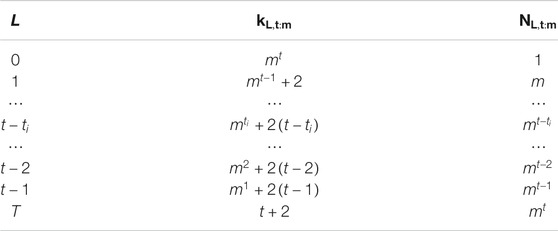
TABLE 1. Degree spectrum.

On the basis of the aforementioned Table 1 and Eq. 4, the dependence of the cumulative distribution $P_{cum}\left(k\ge k_{L,t:m}\right)$ on the degree $k_{L,t:m}$ and the step t is captured by the following equation:

$P_{cum}\left(k\ge k_{L,t:m}\right)=\{\begin{array}{cc}{k}_{L,t:m}^{-{\gamma }_{\alpha }}& m^{t_i}>2\left(t-t_i\right)\\ e^{-\lambda k_{L,t:m}}& m^{t_i}\le 2\left(t-t_i\right)\end{array},(5)$

where power-law exponent ${\gamma }_{\alpha }=1$. Taking the derivative of both sides of k in Eq. 5 yields

$P\left(k\right)=k^{-\gamma },\gamma ={\gamma }_{\alpha }+1=2(6)$

The detailed calculation process of cumulative degree distribution is presented in Appendix. The cumulative degree distribution of our networks is composed of two parts, exponential distribution and power-law distribution. Besides, this result does not match the statement in the previous work. Genio believes that there is no network whose power-law exponent belongs to $0<\gamma \le 2$ in the limitation of the large number of vertices in [18]. Timar et al. explore two models of scale-free networks that have the degree distribution exponent $\gamma =1$[8]. Courtney et al. present a modeling framework which produces networks that are both dense and have scale-free properties in [9]. In addition, in [19], Ma et al. propose a framework for producing scale-free networks with the dense feature using two operations, that is, first-order subdivision and line operation. However, our approach is different from those in the above methods for constructing scale-free networks with dense properties. Meanwhile, the lights shed by them may be helpful to construct some novel networks with certain constraints. Next, we will discuss the small-world property of our networks.

Small-world property: Watts and Strogatz proposed the small-world property of complex networks by using two features: a relative smaller diameter and a higher clustering coefficient [6]. The small-world property of our networks is still not well discussed; despite that, they well describe these two important parameters of topological structures. In the coming discussion, we focus on the diameter and clustering coefficient of our networks.

Diameter: The distance between two vertices is the smallest number of edges to get from u to v. The longest shortest path between all pairs of vertices is called the diameter. The diameter is itself a feature of network structure and can be applied to characterize a communication delay over a network. In general, the larger the diameter is, the lower the communication efficiency is. The diameter of our network is denoted as $D\left(t;m\right)$. Fortunately, for our networks, it can be calculated easily. Here, we will introduce the main computation of the diameter. With the help of the construction process of network $N\left(t;m\right)$, we have

$D\left(t;m\right)=4=O\left(1\right).(7)$

We give an exhaustive calculation process of diameter in Appendix. The reason comprises two main cases: 1) all vertices of the layer $L=t$ are connected to that active vertex of the highest layer, that is, $L=0$; 2) each vertex in the middle layers, $L=1,\dots ,L=t-1$, always attaches to a vertex of the lowest layer, that is, $L=t$. In fact, the diameters $D\left(t;m\right)$ are equal to the distance between two vertices, both of which are in the middle layers and in different branches of network $N\left(t;m\right)$. This forces the network into an active vertex and unit in which all vertices are close to each other because they all connect to the active vertex. In this regime, the diameter is independent of t and m. Note that this $D\left(t;m\right)$ actually is not very large, implying that our networks also have an ultrasmall diameter—two randomly chosen vertices are connected by a fairly short path length. Hence, formally, $D\left(t;m\right)=4;$ for any $t\ge 0$, the diameter is small and far less than the number of vertices. So, we have a surprising result of an ultrasmall diameter in this sense.

Clustering coefficient: The clustering coefficient is another vital property of a network, which provides the measure of the local structure within the network. The most immediate measure of clustering is the clustering coefficient $C_i$ for every vertex i. By definition, the clustering coefficient of a vertex i is the ratio of the total number $E_i$ of edges that actually exist between all $k_i$ (its nearest neighbors) and the number of $k_i\left(k_i-1\right)/2$ of all possible edges between them, that is, $C_i=2E_i/\left[k_i\left(k_i-1\right)\right]$. The clustering coefficient $\langle C\rangle$ of the entire network can be defined as the average of all vertex C’s as follows:

$\langle C\rangle =\frac{{\displaystyle {\sum }_{v\in V}{C}_v}}{\left|V\right|}.(8)$

The clustering coefficient of a vertex i in our networks is as follows:

$C_i\left(k\right)\propto k^{-1}.(9)$

The detailed process of the clustering coefficient will be given in Appendix. The degree of the clustering coefficient of a whole network is captured by the average value of the clustering coefficient, $\langle C\left(t;m\right)\rangle$, representing the average of $C_i$ over all vertices $i=\mathrm{1,2},\dots ,\left|V\left(t;m\right)\right|.$

$\langle C\left(t;m\right)\rangle =\frac{{\displaystyle {\sum }_{i=1}^t\frac{2\left(m^{t-i}+2i\right)m^i}{\left(m^{t-i}+2i\right)\left(m^{t-i}+2i-1\right)}+\frac{2\left(m-1\right)m^t}{\left(t+2\right)\left(t+1\right)}}}{\left|V\left(t;m\right)\right|}.(10)$

Taking the limit on the number of vertices, the clustering coefficient $\langle C\left(t;m\right)\rangle$ of Eq. 10 approaches to a nonzero value, as shown in Figure 3. So we can say that our networks have a high clustering coefficient.

FIGURE 3

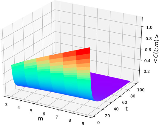
FIGURE 3. Diagram of the clustering coefficient $\langle C\left(t;m\right)\rangle$ of network $N\left(t;m\right)$.

Consequently, our networks, with a smaller diameter and a higher clustering coefficient, can be considered as small-world networks.

Mean first-passage time: In this subsection, we have an attempt to study the trapping problem on our network $N\left(t;m\right)$. Indeed, what is considered here is a simple unbiased discrete-time Markovian random walk with a single trap, namely, an ideal absorber located at a specified vertex on a network. As previously discussed, that active vertex of network$N\left(t;m\right)$ at the step t has the largest degree, referred to as $a_t$. For the sake of convenience, let the active vertex $a_t$ be the trap vertex. At each time step, a walker starting from its current position v moves to one of its neighbors $N_v$ with the transition probability $1/d_v\left(t;m\right)$ before visiting the absorber, where $d_v\left(t;m\right)$ is the number of its existing edges of v in network $N\left(t;m\right)$.

Here we think a walker starts from the vertex v at the initial time. Obviously, we can obtain the fact that the transition probability $P_{vu}$ of starting out from v to reach u holds the following equation:

$P_{vu}\left(l+1\right)={\displaystyle \sum _{i\in V\left(t;m\right)}\frac{a_{iu}}{d_i\left(t;m\right)}}{P}_{vi}\left(l\right),(11)$

where $a_{iu}$ is the entry of the adjacency matrix of network$N\left(t;m\right):$$a_{iu}=1$ if there is an edge connecting vertices i and u, and $a_{iu}=0$ otherwise.

Armed with the rule mentioned above, we want to discuss the most important quantity for the trapping problem, generally named the first-passage time $FPT$. The first-passage time is the expected number of steps for a walker, starting from the vertex v to first arrive at the trap in the trapping problem. For our network $N\left(t;m\right)$, we represent the first-passage time for a walker located in the vertex v by $FP{T}_v$ and let $P\left(FP{T}_v=l\right)$ be the probability for that vertex v to first drop into the trap, namely, the active vertex $a_t$. Similar to Eq. 11, we have

$P\left(FP{T}_v=l\right)={\displaystyle \sum _{\begin{array}{l}i\in V\left(t;m\right),\\ i\ne a_t\end{array}}\frac{a_{iu}}{d_i\left(t;m\right)}P\left(FP{T}_v=l-1\right)}.(12)$

The classical method to solve the aforementioned equation is the generating function. Without loss of generality, we can write down the corresponding generating function of $P\left(FP{T}_v=l\right)$ as follows:

${\mathrm{}}_v\left(x\right)={\displaystyle \sum _{t=0}^{\infty }P\left(FP{T}_v=l\right)x^l}.(13)$

A trial yet helpful fact associated with ${\mathcal{P}}_v\left(x\right)$, the expected time $FP{T}_v,$ is exactly equal to the value $\mathcal{P}{\prime }_v\left(1\right)$, as we will explain shortly in the coming discussion.

Before proceeding further, we first define two notations, $P_t\left(s\right)$ and $Q_L\left(s\right)$. Let $P_t\left(s\right)$ denote the probability for a walker on any vertex at the layer $L=t+1$ of network $N\left(t;m\right)$ to first visit the active $a_t$ after s steps and $Q_L\left(s\right)$ represent the probability that a walker starting from any vertex w at the layer $L\left(L=\mathrm{1,2},\dots ,t\right)$ hits one at a randomly chosen vertex at the layer $L=t+1$ of network $N\left(t;m\right)$, which connects to vertex w, after s steps. Combined with the structure of network $N\left(t;m\right)$ and the statement above, we arrive at the explicit equation for $P_t\left(s\right)$ on our networks as follows:

$P_t\left(s\right)=\frac{{\delta }_{s,1}+{\displaystyle {\sum }_{L=1}^t{\displaystyle {\sum }_{i=1}^{s-1}{Q}_L\left(s\right)P_t\left(s-1-i\right)}}}{k_{L=t+1}},(14)$

where ${\delta }_{s,1}$ is the Kronecker delta function defined as ${\delta }_{s,1}=1$ if s is equal to one and ${\delta }_{s,1}=0;$ otherwise, $k_{L=t+1}$ is the number of edges associated with the vertex at the layer $L=t+1$ and equals $t+1$.

Then, together with Eq. 13, the generating function ${\mathcal{P}}_t\left(x\right)$ corresponding to $P_t\left(s\right)$ can be written as

${\mathcal{P}}_t\left(x\right)=\frac{x}{k_{L=t+1}}+\frac{t{x}^2}{k_{L=t+1}}{\mathcal{P}}_t\left(x\right)(15)$

in which we apply a result $Q_L\left(i\right)=1$ only for both $L=1,\dots ,t$ and $i=1$and $Q_L\left(i\right)=0$ otherwise.

Meanwhile, let $FP{T}_{t+1}^t$ represent the first-passage time for a walker originally placed on any vertex at the layer $L=t+1$ which can be expressed as

$FP{T}_{t+1}^t=\frac{d}{dx}{{\mathcal{P}}_t\left(x\right)|}_{x=1}.(16)$

On the basis of Eq. 16, doing the derivative of both sides of Eq. 15 evolves the exact solution of $FP{T}_{t+1}^t$. It is represented as

$FP{T}_{t+1}^t=2t+1.(17)$

For each vertex at the layer $L=1,\dots ,t$, together with the definition of $Q_L\left(s\right)$ and the hierarchical structure of networks $N\left(t;m\right)$, the first-passage time $FP{T}_L^t$ for a walker formerly set on an arbitrary vertex at the layer L can be expressed in terms of $FP{T}_{t+1}^t.$

$FP{T}_L^t=FP{T}_{t+1}^t+1.(18)$

Then, the first-passage time $FP{T}_L^t$ for a walker at the layer $L=1,\dots ,t+1$ can be computed in a sharp mode. Our next purpose is to deduce the mean first-passage time ${\langle FTP\rangle }_t$, which depicts the trapping process with a random walk on average.

${\langle FTP\rangle }_t=\frac{1}{\left|V\left(t;m\right)-1\right|}{\displaystyle \sum _{L=1}^{t+1}FP{T}_L^t\left|N_t\left(L\right)\right|}.(19)$

Here, we again apply the hierarchical structure of network $N\left(t;m\right)$, and $\left|N_t\left(L\right)\right|$ represents the total number of vertices at the layer $L\left(L=1,\dots ,t+1\right)$. As previously stated, we find that $\left|N_t\left(L\right)\right|$ is equal to $N_{L,t;m}$.

Plugging Eqs 17 and 18 and the value of $\left|V\left(t;m\right)\right|$ into Eq. 19, we obtain the subsequent equation by taking advantage of several simple mathematics

${\langle FPT\rangle }_t=O\left(2t+\frac{1}{m}\right).(20)$

Moreover, we think the logarithm of the number of vertices of network $N\left(t;m\right)$, that is, $\ln \left|V\left(t;m\right)\right|\sim \left(t+1\right)\ln m$. It is straightforward to discover that for the entire network $N\left(t;m\right)$, the mean first-passage time ${\langle FPT\rangle }_t$ is closely related to the number of vertices of network $N\left(t;m\right).$

${\langle FPT\rangle }_t\sim \ln \left|V\left(t;m\right)\right|.(21)$

Thus, in the large limit of the number of vertices of network$N\left(t;m\right)$, the mean first-passage time increases logarithmically with the number of vertices of our networks. Equation 21 reveals the relationship of the mean first-passage time on the number of edges of our networks. Figure 4 describes the fact that the mean first-passage time is a function of step t.

FIGURE 4

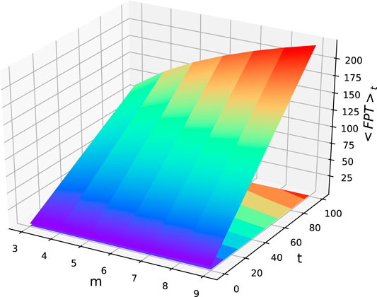
FIGURE 4. Diagram of the mean first-passage time ${\langle FPT\rangle }_t$ of network $N\left(t;m\right)$.

This is a bit different from some previous results in the existing literature; for instance, for a complete graph with N vertices, the mean first-passage time is exactly equal to $N-1$, which scales linearly with the number of vertices. One can see that the mean first-passage time of the Apollonian network increases as a fractional power of the number of vertices, which implies that the Apollonian network has a faster transmit time than any other analytically soluble media [20]. In contrast to our networks, the complete graph has no scale-free feature and hierarchical structure, but has the ultrasmall diameter and dense feature. On the other hand, the Apollonian network has a larger diameter than our networks, which indicates the scale-free feature and hierarchical structure. All things considered, it may be safely said that our network $N\left(t;m\right)$ outperforms those networks in [20] with respect to the mean first-passage time in the trapping problem.

3 Conclusion and Discussion

In our article, we present a class of scale-free networks with the dense feature. On the basis of our analysis, we deduce some striking results.1) The average degree of our networks is not approximately a fixed constant value, and its value diverges with the step t, and then we reveal the fact that our networks are dense. 2) The cumulative degree distribution of our networks $N\left(t;m\right)$ contains two parts: exponential degree distribution and power-law distribution with the exponent $\gamma =2$. 3) Combined with the diameter and clustering coefficient, we hold the opinion that our networks have the small-world effect. 4) The mean first-passage time in network $N\left(t;m\right)$ is approximately related to the logarithm number of vertices of networks. Our findings are insightful for the study of the random walks on various deterministically growing networks. Our work creates a broader perspective on previous research studies of trapping on diverse networks and sheds light on some aspects related to the trapping problem, providing some relationship information between efficiency and underlying the network size. In the future, we hope that the current study can provide some inspiration for trapping problems in real networks with topologies similar to ours.

Data Availability Statement

The original contributions presented in the study are included in the article/supplementary Material; further inquiries can be directed to the corresponding author.

Author Contributions

XW provided this topic and wrote the paper. FM discussed and modified it, and BY guided the manuscript. All authors contributed to manuscript and approved the submitted version.

Funding

This research was supported in part by the National Key Research and Development Program of China under Grant No. 2019YFA0706401; in part by the National Natural Science Foundation of China under Grant No. 61632002; in part by the General Program of the National Natural Science Foundation of China under Grant No. 61872399, Grant No. 61872166, and Grant No. 61672264; in part by the Young Scientists Fund of the National Natural Science Foundation of China under Grant No. 61802009, Grant No. 61902005, and Grant No. 62002002; and in part by the National Natural Science Foundation of China under Grant No. 61662066.

Conflict of Interest

The authors declare that the research was conducted in the absence of any commercial or financial relationships that could be construed as a potential conflict of interest.

References

1. Ravasz E, Barabási AL. Hierarchical organization in complex networks. Phys Rev E (2003) 67:026112. doi:10.1103/physreve.67.026112

PubMed Abstract | CrossRef Full Text | Google Scholar

2. Fornito A, Zalesky A, Breakspear M. The connectomics of brain disorders. Nat Rev Neurosci (2015) 16:159–172. doi:10.1038/nrn3901

PubMed Abstract | CrossRef Full Text | Google Scholar

3. Iranzo J, Buldú JM, Aguirre J. Competition among networks highlights the power of the weak.Nat Commun (2016) 7:13273. doi:10.1038/ncomms13273

PubMed Abstract | CrossRef Full Text | Google Scholar

4. Mocanu DC, Exarchakos G, Liotta A. 2004 IEEE international conference on systems, man, and cybernetics; 2004 Oct 10–13; The Hague, Netherlands. (2014). p. 19–24.

5. Albert R, Jeong H, Barabási A-L. Error and attack tolerance of complex networks. Nature (2000) 406:378–382. doi:10.1038/35019019

PubMed Abstract | CrossRef Full Text | Google Scholar

6. Watts DJ, Strogatz SH. Collective dynamics of “small-world” networks. Nature (1998) 393:440–2. doi:10.1038/30918

PubMed Abstract | CrossRef Full Text | Google Scholar

7. Barabási A-L, Albert R. Emergence of scaling in random networks. Science (1999) 286:509–12. doi:10.1126/science.286.5439.509

PubMed Abstract | CrossRef Full Text | Google Scholar

8. Timár G, Dorogovtsev SN, Mendes JFF. Scale-free networks with exponent one. Phys Rev E (2016) 94:022302. doi:10.1103/physreve.94.022302

PubMed Abstract | CrossRef Full Text | Google Scholar

9. Courtney OT, Bianconi G. Dense power-law networks and simplicial complexes. Phys Rev E (2018) 97:052303. doi:10.1103/physreve.97.052303

PubMed Abstract | CrossRef Full Text | Google Scholar

10. Barabási A-L, Albert R, Jeong H. Mean-field theory for scale-free random networks. Physica A: Stat Mech its Appl (1999) 272:173–87. doi:10.1016/s0378-4371(99)00291-5

CrossRef Full Text | Google Scholar

11. Newman MEJ, Moore C, Watts DJ. Mean-field solution of the small-world network model. Phys Rev Lett (2000) 84(14):3201–4. doi:10.1103/physrevlett.84.3201

PubMed Abstract | CrossRef Full Text | Google Scholar

12. Newman MEJ, Strogatz SH, Watts DJ. Phys Rev E (2000) 64:026118.

13. Krapivsky PL, Redner S, Leyvraz F. Connectivity of growing random networks. Phys Rev Lett (2000) 85(21):4629–32. doi:10.1103/physrevlett.85.4629

PubMed Abstract | CrossRef Full Text | Google Scholar

14. Krapivsky PL, Rodgers GJ, Redner S. Degree distributions of growing networks. Phys Rev Lett (2001) 86(23):5401. doi:10.1103/physrevlett.86.5401

PubMed Abstract | CrossRef Full Text | Google Scholar

15. Barabási AL. Network science. Cambridge, United Kingdom: Cambridge University Press (2016). p. 10–3.

16. Barabási A-L, Ravasz E, Vicsek T. Deterministic scale-free networks. Physica A: Stat Mech its Appl (2001) 299:559–64. doi:10.1016/s0378-4371(01)00369-7

CrossRef Full Text | Google Scholar

17. Dorogovtsev SN, Goltsev AV, Mendes JFF. Pseudofractal scale-free web. Phys Rev E (2002) 65:066122. doi:10.1103/physreve.65.066122

PubMed Abstract | CrossRef Full Text | Google Scholar

18. Del Genio CI, Gross T, Bassler KE. All scale-free networks are sparse. Phys Rev Lett (2011) 107:178701. doi:10.1103/physrevlett.107.178701

PubMed Abstract | CrossRef Full Text | Google Scholar

19. Ma F, Wang XM, Wang P, Luo XD. Dense networks with scale-free feature. Phys Rev E (2020) 101:052317. doi:10.1103/physreve.101.052317

PubMed Abstract | CrossRef Full Text | Google Scholar

20. Zhang Z, Guan J, Xie W, Qi Y, Zhou S. Random walks on the Apollonian network with a single trap. Europhys Lett (2009) 86:10006. doi:10.1209/0295-5075/86/10006

CrossRef Full Text | Google Scholar