Single-Shot Through-Focus Image Acquisition and Phase Retrieval From Chromatic Aberration and Multi-Angle Illumination

Introduction

Quantitative phase imaging (QPI) [1] is crucial to label-free microscopic imaging in biomedical fields. In general, for light field passing through a transparent sample, the phase modulation caused by the sample refractive index distribution carries more effective information than the intensity modulation caused by the sample absorption distribution. Nevertheless, instead of phase distributions, we can only obtain intensity distributions with any existing photodetectors due to the extremely fast oscillations of light. Since the early 1900s, a lot of phase imaging methods converting phase to intensity measurement have been proposed [2–7]. It can be roughly classified into two categories. One is contrast phase measurement methods, such as phase-contrast microscopy [8]. Another one is quantitative phase measurement, including interferometry [9], Shack–Hartmann wave front sensor (SHWFS) [10, 11], and so on. The measurement accuracy of interferometry is high, but it is sensitive to environmental noises and suffers from an unwrapping problem. Compared with interferometry, SHWFS and phase-contrast microscopy have relatively simple system constructions and superior anti-jamming characteristics, but the measurement accuracy of SHWFS is relatively low and phase-contrast microscopy can only achieve a qualitative phase. Therefore, phase imaging with the characteristics of simple structure and strong robustness to noise and environmental disturbances has always been pursued by researchers.

Compared with the conventional methods mentioned above, phase retrieval methods rooting in diffraction have been used widely due to their high anti-jamming capability and good performance, including Fourier ptychographic imaging (FPM) [12–14], ptychographic iterative engine (PIE) [15–18], and so on. PIE aims to retrieve the phase distribution from a series of diffraction patterns corresponding to illumination situations with different positions but a certain overlap ratio between adjacent illumination probes. FPM, sharing its root with phase retrieval and synthetic aperture imaging, can realize a high-resolution (HR), large field-of-view (FOV) amplitude and phase of an object simultaneously. Although PIE and FPM are widely used in quantitative phase imaging, a key problem involved is the time-consuming data acquisition process. In comparison, some phase retrieval methods based on through-focus diversity have also been proposed. Transport of intensity equation (TIE) [19–23] can realize robust phase recovery by constructing the relationship between phase distribution and the differential of light distribution along the optical axis. The axial intensity differential can be equivalent realized by the difference between two through-focus intensity images. Different from the above strategy that calculates phase distribution directly from clear physical models, another kind of phase imaging strategy is realized through the optimization strategy of round-trip iterative constraints between two or more through-focus intensity images. Typical optimization algorithms include the Gerchberg–Saxton (GS) rooting in alternating projection (AP) or projection onto convex sets (POCS), averaged projection, averaged reflection and relaxed averaged alternating reflection (RAAR), etc. [24]. Nevertheless, both TIE and iteration optimization methods need to mechanically scan a camera or sample to obtain the through-focus intensity images, which relies on a precision mechanical moving device.

In order to avoid mechanical scanning and reduce data acquisition time, several methods based on single-shot through-focus intensity image acquisition have been proposed. For example, Waller et al. used chromatic aberration of objective to acquire three raw images simultaneously [25]. Komuro et al. realized TIE phase retrieval with multiple bandpass filters [26] and polarization-directed flat lenses [27, 28]. However, the above methods still require precise mechanical movement calibration of the defocus distance of the system in advance, which is complicated and time-consuming. What is more, the relative distances between each color channel are also related to the overall defocus distance of the sample, which cannot be obtained in a single measurement.

In this paper, we propose a single-shot phase retrieval method based on chromatic aberration and image lateral shift resulting from the multi-angle illuminations of the out-of-focus sample. A sample located at a defocus position is illuminated by light sources of different wavelengths from different incident angles and then imaged with an RGB (red, green, blue) color camera through a microscopic objective. Due to the chromatic aberration of the objective and the different illumination angles, three monochromatic intensity images (red, green, and blue) can be extracted from a single-frame color image. By calculating the lateral shift of each section of the sample, the relative defocus distance between the focus plane and the channel planes can be obtained mathematically. Benefiting from this strategy, defocus distances can be obtained easily without any mechanical moving device and precise measurement. Then, the AP phase retrieval algorithm is utilized to realize phase distribution recovery. Lastly, three-dimensional (3D) localization of the sample can also be obtained. Furthermore, we also improve the Fresnel transfer function (TF) propagator in the AP phase retrieval algorithm in order to accommodate the angle-varied illuminations and out-of-focus samples. This paper is organized as follows: the optical imaging model with angle-varied illuminations is presented in section Oblique Illumination Model. The SAD image registration method used for calculating the image lateral shift is presented in section SAD Image Registration. Color cross-talk in the RGB camera and the AP phase retrieval framework with improved Fresnel TF propagator are presented in sections Color Cross-Talk Elimination and Alternating Projection Phase Retrieval Algorithm, respectively. Section Simulation Experiment presents the simulations to demonstrate the feasibility of the proposed method. We use biological samples in section Experiments to prove the success of phase retrieval experimentally. Finally, the conclusion and discussion are summarized in section Conclusion and Discussion.

Principle

Oblique Illumination Model

As shown in Figure 1, we build a model to illustrate how the defocus distance and illumination angles affect the image lateral shift in microscopy. If a sample is placed at an out-of-focus position, the images corresponding to illuminations from different angles will have a relative lateral shift between each other. Zheng et al. also realized auto-focusing for microscopic imaging with the lateral shift amount as a defocus distance criterion [29].

FIGURE 1

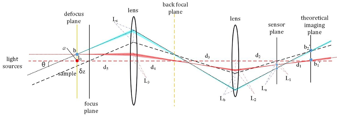
Figure 1. Oblique illumination out-of-focus sample imaging model.

A sample is placed at a defocus plane and illuminated by two light beams with the same wavelength, but different incident angles simultaneously, as shown in Figure 1. δz is the defocus distance and θ is the angle between two incident light sources. d₁ is the distance between the sensor plane and the theoretical imaging plane. d₂, d₃, d₄, and d₅ are system parameters corresponding to the microscopic system. Assuming there are two points of the sample, a and b. a locates at the optical axis, and the distance between a and b is l₀. ${b_1}^{\prime }$ and ${b_2}^{\prime }$ are two imaging points corresponding to point b with different incident angles at the theoretical imaging plane. If the sample is placed at the focus plane, both axial points and off-axis points have no lateral shift at the theoretical imaging plane. Thus, ${b_1}^{\prime }$ and ${b_2}^{\prime }$ will coincide at the theoretical imaging plane. But if the sample is placed at an out-of-focus plane, a lateral shift between ${b_1}^{\prime }$ and ${b_2}^{\prime }$ will appear. As shown in Figure 1, the lateral shift between ${b_1}^{\prime }$ and ${b_2}^{\prime }$ at the sensor plane is defined as δL = L_a − L₁. We can derive some equations connecting the above-mentioned variables together.

$\begin{array}{ll}\{\begin{array}{c}\frac{L_1}{L_2}=\frac{d_1}{d_1+d_2}\\ \frac{L_2}{L_3}=\frac{d_3}{d_4}\\ L_3=l_0\end{array},\{\begin{array}{c}\frac{L_a}{L_b}=\frac{d_1}{d_1+d_2}\\ \frac{L_b}{L_c}=\frac{d_3}{d_4}\\ L_c=l_0+\delta z·tan\theta \end{array}.& (1)\end{array}$

Equation (1) can be further organized as follows:

$\begin{array}{ll}\text{δL}=L_a-L_1=\frac{d_1·d_3}{d_4·(d_1+d_2)}·tan\theta ·\delta z=\xi ·tan\theta ·\delta z& (2)\end{array}$

where $\xi =\frac{d_1·d_3}{d_4·(d_1+d_2)}$ is a constant value corresponding to each specific wavelength. It will have different values for different wavelengths due to the chromatic aberration characteristics of the objective. Essentially, Equation (2) aims to calculate the defocus distance δz from d₁. Due to the microscopy and the camera forming an integrated system, the axial defocus distance d₁ is difficult to measure directly. Therefore, we transform calculating d₁ to the lateral distance δL in Equation (2). Given that the AP algorithm framework requires at least two through-focus intensity images to be implemented, we utilize three-wavelength light-emitting diodes (LEDs) corresponding to the three channels of the RGB camera to illuminate the out-of-focus sample from different directions respectively. As shown in Figure 2, a red LED is placed at the optical axis, and the corresponding defocus image is used as a reference value because of the characteristic that the defocus image illuminated by normal incidence illumination will not have a lateral shift relative to the focused image. One green LED and one blue LED are placed at the two off-axis positions to provide oblique illuminations, in which the incident illumination angles are θ_rg and θ_rb, respectively. The defocus distances δz_fg and δz_fb between the focus plane and the green/blue channel images can be calculated through Equation (3). We should emphasize that benefiting from the normal incidence illumination corresponding to red LED, although the red channel image is located at the out-of-focus position, there exists no lateral shift compared with the focus image. The red channel image can be used as a reference value to calculate the defocus distances between the focus plane and the green/blue channel images. Therefore, we transform calculating the lateral shift between the focus image and the green/blue channel image to calculating the lateral shift between the red and green/blue channel images. Equation (3) indicates that the lateral shifts of the green and blue channels relative to the red image are proportional to the defocus distances between the focus plane and the green/blue channel image, where A_ri is a constant value decided by the incident angle and wavelength.

$\begin{array}{ll}\text{δ}{\text{L}}_{ri}={\xi }_{ri}·tan{\theta }_{ri}·\text{δ}{z}_{fi}=A_{ri}·\text{δ}{z}_{fi},(i=g,b)& (3)\end{array}$

FIGURE 2

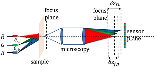
Figure 2. Single-shot oblique illuminations system of our method.

SAD Image Registration

According to the above-mentioned illumination direction and the wavelength multiplexing strategy in section Oblique Illumination Model, we can obtain the defocus distances by calculating the lateral shifts between the red and green/blue channel images. To obtain the precise shifts between different images, we use the sum of absolute differences (SAD) to realize image matching [30, 31]. SAD is a widely used, extremely simple video quality metric used for block matching in motion estimation for video compression. It works by taking the absolute value of the difference between each pixel in the original block and the corresponding pixel in the block being used for matching. As shown in Equation (4), S(i + s − 1, j + t − 1) is one pixel value of the original block and T(s, t) is the corresponding pixel in the block for comparison.

$\begin{array}{l}\text{D}(i,j)={\displaystyle \sum _{s=1}^M}{\displaystyle \sum _{t=1}^N}|S(i+s-1,j+t-1)-T(s,t)|,\\ (1\le i\le m-M+1,1\le j\le n-N+1)& (4)\end{array}$

We show a simulation example of the SAD image registration strategy in Figure 3. Figures 3A,C are the original and comparison images, respectively. A window block in Figure 3A is enlarged, as shown in Figure 3B, whose coordinates of the top left corner is (300, 100). Then, we search for window blocks in different positions in Figure 3C and calculate the SAD value between them and Figure 3B. Finally, we can find the optimal block, whose coordinates of the top left corner is (270, 100). The red boxed sub-region in Figure 3C, owning the minimum SAD value with Figure 3B, is the best-matched block corresponding to Figure 3B. The relative pixel position shift between the matching block pair is (−30, 0), which is consistent with the set value. Assigning a value to pixel size, we can calculate the defocus distance according to Equation (3). Given the discrete sampling process of a digital camera sensor, Equation (3) can be rewritten as follows:

$\begin{array}{ll}\text{δ}{\text{L}}_{ri}={Ps}_{ri}·S_p=A_{ri}·\text{δ}{z}_{fi},(i=g,b)& (5)\end{array}$

where Ps_ri is the pixel shift between the red channel and the green/blue channels and S_p is the pixel size of the RGB camera we used in the following experimental section.

FIGURE 3

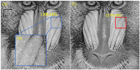
Figure 3. Sum of absolute differences (SAD) image registration examples. (A) Original image. (B) Window block used for image matching. (C) Comparison image in which there is a −30-pixel shift corresponding to the x coordinate between (A) and (C).

Color Cross-Talk Elimination

Generally speaking, the most common color industrial camera is combined with a Bayer filter and a complementary metal oxide semiconductor (CMOS) sensor. However, due to the color separation performance of the Bayer filter being imperfect, color cross-talk or color leakage will exist among each of the color channels (i.e., red, green, and blue) [32, 33]. Thus, eliminating the color cross-talk among the RGB channels before separating them is important in our proposed method. The imaging process of RGB oblique illumination with a color camera can be mathematically described as follows:

$\begin{array}{ll}\left[\begin{array}{c}{M}_R\\ M_G\\ M_B\end{array}\right]=\text{W}·\left[\begin{array}{c}{I}_r\\ I_g\\ I_b\end{array}\right]=\left[\begin{array}{ccc}{R}_r& R_g& R_b\\ G_r& G_g& G_b\\ B_r& B_g& B_b\end{array}\right]·\left[\begin{array}{c}{I}_r\\ I_g\\ I_b\end{array}\right]& (6)\end{array}$

where W is the color cross-talk matrix between the RGB channels. M_R, M_G, and M_B are the RGB channels captured by the color camera, and the subscripts R, G, and B indicate the red, green, and blue channels, respectively. I_r, I_g, and I_b are the illumination intensities in front of the Byer filter corresponding to red, green, and blue colors, respectively. The illumination parameters in the color cross-talk matrix W can be obtained experimentally by a spectrometer or calculated using Equation (7), where the superscript “−1” refers to the inverse matrix.

$\begin{array}{ll}\text{W}=\left[\begin{array}{ccc}{R}_r& R_g& R_b\\ G_r& G_g& G_b\\ B_r& B_g& B_b\end{array}\right]=\left[\begin{array}{c}{M}_R\\ M_G\\ M_B\end{array}\right]·{\left[\begin{array}{c}{I}_r\\ I_g\\ I_b\end{array}\right]}^{-1}& (7)\end{array}$

In our experiment, a color camera (FLIR, BFS-U3-200S6C-C) is used for recording images. The matrix W corresponding to the wavelengths of the RGB LED (470, 517, and 626 nm, respectively) is shown in Table 1.

TABLE 1

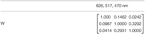
Table 1. Color cross-talk matrix W of our RGB camera.

Alternating Projection Phase Retrieval Algorithm

Alternating projection is a kind of optimization strategy realized by sequentially projecting onto several constraints back and forth multiple times. It has been utilized in performing phase retrieval by means of through-focus intensity images [34, 35]. The simplest case of AP involves two constraints, curves A and B, as shown in Figure 4. The intersection point x^* of two constraints indicates the optimal solution of this case. The AP framework can start with an initial guess, x₀, and then projecting x₀ between constraints A and B sequentially. The optimal solution x^* can be found finally as shown in Figure 4. Actually, in real experiments, three or more physical constraints can be utilized in the AP process to help improve the possibility of jumping out of the local optimal solution and increase the convergence efficiency, which is also named “sequential projection” or “cyclic projection.”

FIGURE 4

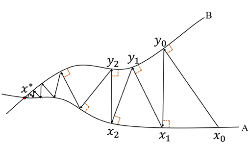
Figure 4. Alternating projection between constraints A and B.

The information of a sample under test can be represented by a 3D transmittance distribution, which can be written as Equation (8).

$\begin{array}{ll}U(\vec{r})=A_m·e^{j·\vec{k}·\vec{r}}& (8)\end{array}$

where A_m is the amplitude transmittance of the object and $e^{j·\vec{k}·\vec{r}}$ refers to the phase transmittance part. $k=\frac{2·\pi }{\lambda }$ is the wave vector, where λ indicates the illumination wavelength. Vector $\vec{r}$ denotes the 3D position. Combining with the Fresnel TF propagator, we can propagate the complex light field to different positions and obtain several field distributions corresponding to the different defocus distances [36]. A common propagation routine can be expressed as Equation (9).

$\begin{array}{ll}{U}_2(x,y)=I^{-1}\{I\{U_1(x,y)\}H(f_x,f_y)\}& (9)\end{array}$

where (x, y) indicates a 2D plane, U₁(x, y) is the original field distribution, and U₂(x, y) is the field in a distance observation plane. The transfer function H is described as Equation (10), where z is the propagation distance from the U₁(x, y) plane to the U₂(x, y) plane.

$\begin{array}{ll}H(f_x,f_y)=e^{jkz}exp\left[-j\pi \text{λ}z\left(f_x^2+f_y^2\right)\right].& (10)\end{array}$

The propagator H shown in Equation (10) is applied to a wide range of propagation scenarios that accommodate normal incidence illuminations. However, in angle-varied illuminations, if a sample is placed at the defocus plane, oblique illumination will result in not only a lateral shift in the spatial domain but also a spectrum shift in the Fourier domain. Thus, to solve the spectrum shift, the propagator should be improved.

According to the Fresnel TF propagator with angle-varied illuminations, the phase function can be described as shown in Equation (11), where k_x, k_y are components of the wave vector corresponding to the x-axis and y-axis, respectively.

$\begin{array}{ll}\Phi (x,y)=k_{x}x+k_{y}y& (11)\end{array}$

As shown in Figure 5A, $\left|\vec{r}\right|$ is the radial distance in the observation plane from the origin to the beam aiming point and z is the perpendicular distance between two planes. Equation (11) can be rewritten as follows, where $\alpha =ta{n}^{-1}\left(\frac{y}{x}\right)$ and θ indicates the illumination angle.

$\begin{array}{ll}\Phi (k_x,k_y)=z(k_{x}cos\alpha +k_{y}sin\alpha )tan\theta & (12)\end{array}$

FIGURE 5

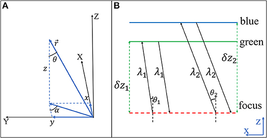
Figure 5. (A) Oblique illumination model in the Fresnel propagation. (B) Alternating projection utilized in the proposed method.

The propagator in our strategy should be improved as Equation (13), where $k_z^2=k^2-k_x^2-k_y^2$.

$\begin{array}{ll}H(k_x,k_y)=e^{j{k}_{z}z}·e^{jz(k_{x}cos\alpha +k_{y}sin\alpha )tan\theta }& (13)\end{array}$

To obtain several constraints in the optical imaging process, we can propagate the complex light field to different positions by the propagator in Equation (13) and record the corresponding intensity image stack. For instance, as shown in Figure 5B, we set α = 0. By utilizing the axial chromatic aberration characteristics, we use two channels (green and blue) of the same planar sensor to record the intensity images corresponding to the different propagation distances with different illumination angles. The perpendicular defocus distance δz_n between the focus plane and the green/blue channels can be calculated by Equation (3). Intensity images obtained with a digital image sensor can directly be expressed as Equation (14).

$\begin{array}{ll}{I}_n=|I^{-1}\{I\{U(x,y)\}{H}_n(k_x,k_y)\}{|}^2,n=1,2,& (14)\end{array}$

where the intensity images I₁, I₂ that correspond to the green and blue channels form two constraints, respectively. H_n(k_x, k_y) is the Fresnel propagator with different illumination angles and distances. Thus, according to Figure 5B, the framework of the alternating projection phase retrieval approach can be expressed as the process shown in Figure 6, where Amplitude_recovered and Phase_recovered are the recovered amplitude and phase of the sample. loopNum is an iteration number (typical values are 10, 20, and so on).

FIGURE 6

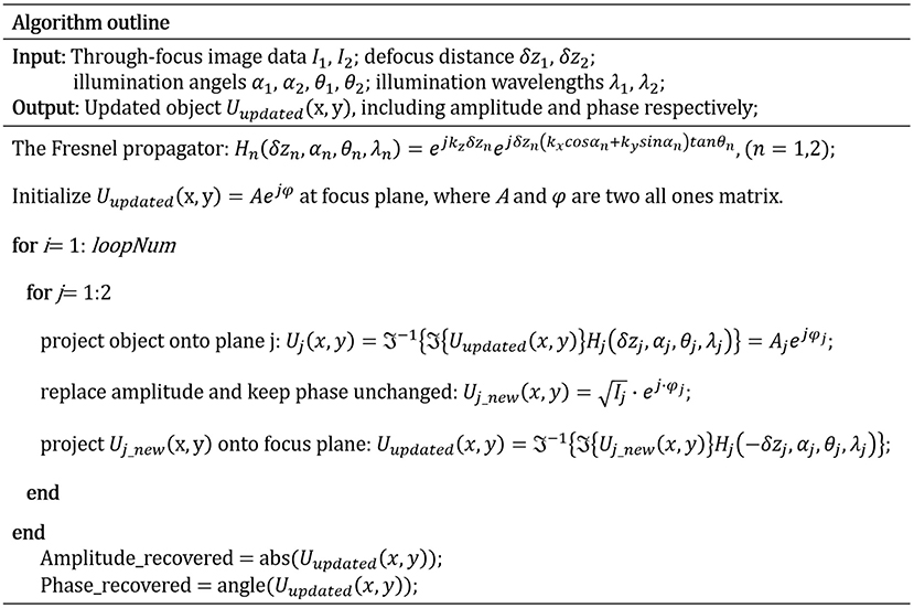
Figure 6. Algorithm outlines of alternating projection in phase retrieval.

Simulation Experiment

Consistent with the systematic parameters in the experiments, the illumination wavelengths are set to 470, 517, and 626 nm in simulation. The pixel size of the RGB camera is 2.4 μm. The distance between the illumination source and the sample plane is 80 mm. According to Figure 2, a red LED unit is placed on the optical axis, in which the corresponding channel image is used as a reference. The x-dimension lateral distance between the red and green LED is set to Dx_rg = 5 mm and the y-dimension distance is set to Dy_rg = 0 mm, which means α is set to 0. In a similar way, we set Dx_rb = 10 mm and Dy_rb = 0 mm, where r, g, and b indicate the red, green, and blue light source, respectively. Therefore, the tangent functions of the illumination direction angles in Figure 2 are ${tan\theta }_{rg}=\frac{5}{80}$ and ${tan\theta }_{rb}=\frac{10}{80}$, respectively. In the simulations, we assume that the scale factor ξ = 1. Thus, Equation (3) can be rewritten as follows:

$\begin{array}{ll}\text{δ}{\text{L}}_{ri}={Ps}_{ri}·S_p={tan\theta }_{ri}·\text{δ}{z}_{fi},(i=g,b)& (15)\end{array}$

As shown in Figures 7A,B, the “baboon” and “rice” images are used as the ground truth of the amplitude and phase parts, respectively. Their image size is set to 512 × 512. By using the Fresnel diffraction equation shown in Equation (14), we obtain three intensity images at different axial positions, as shown in Figures 7C–E. As mentioned above, Figure 7C belongs to the red channel image, which is illuminated by the normal incidence illumination. Thus, Figure 7C is used as the reference to calculate the defocus distances between the focus plane and the green/blue image planes. The equivalent defocus distances between the focus plane and each image plane is set as z_i = [30, 100, 200] um, (i = r, g, b). And the x-dimension separation between the focus plane and each channel image can be written as Lx_i = [0, 6.25, 25]um, (i = r, g, b), according to Equation (15), while the y-dimension separations are 0. Thus, the relative pixel shifts between the red and green/blue channels can be calculated as Ps_ri = [2.6, 10.4] pixels (i = g, b), theoretically. Considering the discrete sampling property of digital cameras, pixel shifts should be rounded as Ps_ri = [3, 10] pixels (i = g, b). In general, Figures 7C–E are the final raw data corresponding to the red, green, and blue channels, respectively, which involve different defocus distances and pixel shifts in our simulations.

FIGURE 7

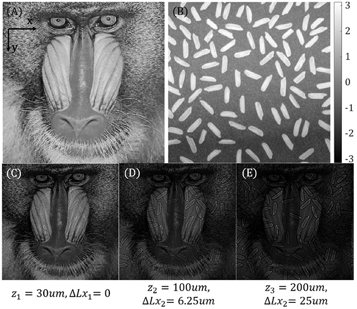
Figure 7. Simulation results. (A) Ground truth of amplitude. (B) Ground truth of phase. (C–E) Raw images with different defocus distances and pixel shifts.

Figure 8 shows the flow diagram of the proposed method. We chose two 64 × 64 window blocks T_g and T_b as comparisons from Figures 7D,E, respectively, which is similar to that in section SAD Image Registration. Then, according to Equation (4), by searching for the optimal window blocks that have the minimum SAD values with T_g and T_b in the red channel intensity image, we can obtain the pixel shifts Ps_rg, Ps_rb between the red channel and the green/blue channels. The absolute defocus distance between the focus plane and the green/blue channels, δz_fg, δz_fb, can be calculated by Equation (15). For example, in our simulations, the pixel shifts we calculated are Ps_rg = 3 pixels and Ps_rb = 10 pixels, which conform to the parameters we simulated. And according to Equation (15), the absolute defocus distances we obtained are δz_fg = 115 um and δz_fb = 192 um, which are approximately equal to the ideal values. This error comes from the round-off operation to non-integer pixel data.

FIGURE 8

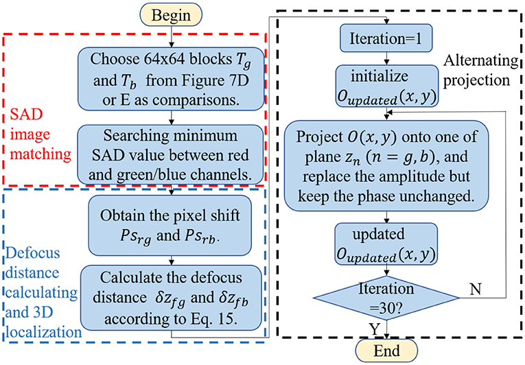
Figure 8. Flow diagram of the proposed method.

In accordance with the defocus distance obtained above, AP phase retrieval approaches are used for phase recovery. According to section Alternating Projection Phase Retrieval Algorithm, two images corresponding to the green and blue channels are used as amplitude constraints, which means that the amplitude of the complex light field to be recovered at the same axial position should be equal to the square root of the image intensity value. We give an initial guess of the sample's complex function firstly at the focus plane, and then projecting it onto the green (or blue) plane position, replacing the amplitude part with the measured value while keeping the phase part unchanged, and then projecting it back to the focus plane. By repeating this procedure, we can obtain an updated object complex function. Through multiple projections and amplitude replacements between the focal plane and the corresponding constraints of the blue and green channels, we can obtain a final solution. The amplitude and the phase part recovered with the above approach are shown in Figure 9. The cross-talk between amplitude and phase may come from the calculation deviation of the SAD and the following error of defocus distance.

FIGURE 9

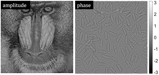
Figure 9. Alternating projection phase retrieval results.

Furthermore, by propagating the recovered object function to the different defocus distances, we can also realize 3D localization in the proposed method. As shown in Figure 10, we propagate the recovered object function to 200, 400, and 800 μm with the illumination angle, θ_rg, and obtain both the amplitude and phase of the sample corresponding to the different defocus distances, respectively. Compared with the amplitude parts of the sample in Figures 10A–C, by changing the different propagation distances but the same incidence illumination angle, we found that our method can be used in refocusing. With the increase of the propagation distance, the lateral shift is clearer in the results. Furthermore, compared with the phase parts of the sample in Figures 10A–C, we found that the phase parts also change with the increase of the propagation distance. Generally, the results shown in Figure 10 demonstrate the feasibility of our method by simulations in 3D localization.

FIGURE 10

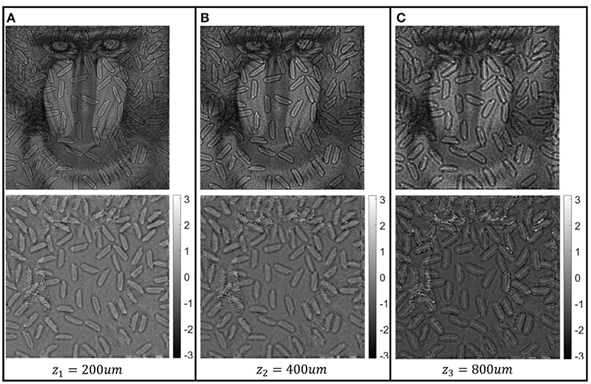
Figure 10. (A–C) Amplitude and phase of the sample corresponding to defocus distances of 200, 400, and 800 μm, respectively.

Experiments

To demonstrate the feasibility of our method in actual experiments, we use Paramecium and bee wing as samples for parameter calibration, phase imaging, and 3D localization. In our experiment, the optical system consists of an RGB camera (FLIR, BFS-U3-200S6C-C) for recording images, a telecentric objective with certain chromatic aberrations (OPTO, TC23004; magnification ×2, NA ≈ 0.1, FOV = 4.25 mm × 3.55 mm, working distance = 56 mm) for imaging, and an RGB LED array (CMN, P = 2.5, 470, 517, and 626 nm) for providing wavelength and direction multiplexing illumination. The system setup is shown in Figure 11A. The distance between the sample plane and the illumination LED plane is adjusted to 90 mm. According to Figure 2, red, green, and blue LEDs are used for angle-varied illuminations. Similar to the parameter set in the simulations, the y-dimension lateral distance between the red and green LEDs is set to Dy_rg = 2.5 mm and the x-dimension distance is set to Dx_rg = 0 mm, which means α is set to 90°. We set Dy_rb = 5 mm and Dx_rb = 0 mm, where r, g, and b indicate the red, green, and blue light sources, respectively. The red illumination light is normally incident onto the sample, while the tangent functions of the illumination angles are ${tan\theta }_{rg}=\frac{2.5}{90}$ and ${tan\theta }_{rb}=\frac{5}{90}$ for the green and blue lights, respectively. Before implementing Equation (3) to calculate the defocus distance for each channel, we should obtain the scale factors A_rg and A_rb first. As shown in Figures 11B–G, we use a Paramecium biological sample to realize the scale factor calibration. Figures 11B–D show the three monochromatic intensity images extracted from the RGB channels of the same image sensor, respectively. Figure 11B is the reference image corresponding to the red channel. Figures 11E,F are two window blocks we choose to search for the minimum SAD value between the red and green/blue channels, respectively. We change the defocus distance from 0 to 600 μm, in which step the size is set to 20 μm and we record the corresponding through-focus images. By implementing the SAD image registration method, we can calculate the pixel shift between the red and green/blue channels. Table 2 is a set of SAD image matching results of the reference image and the blue channel image. As shown in Figure 11G, by using the linear fitting method, we can obtain the scale factor of the two different wavelengths as follows: A_rg = 0.045 and A_rb = 0.071. Then, combining with the results of the scale factor, we can obtain the defocus distance between the focus plane and the green/blue channel planes mathematically. Furthermore, according to Figure 11G, we found that the absolute defocus distances at the 0-pixel shift between the green and blue channels are different, which is caused by the chromatic aberration of objectives.

FIGURE 11

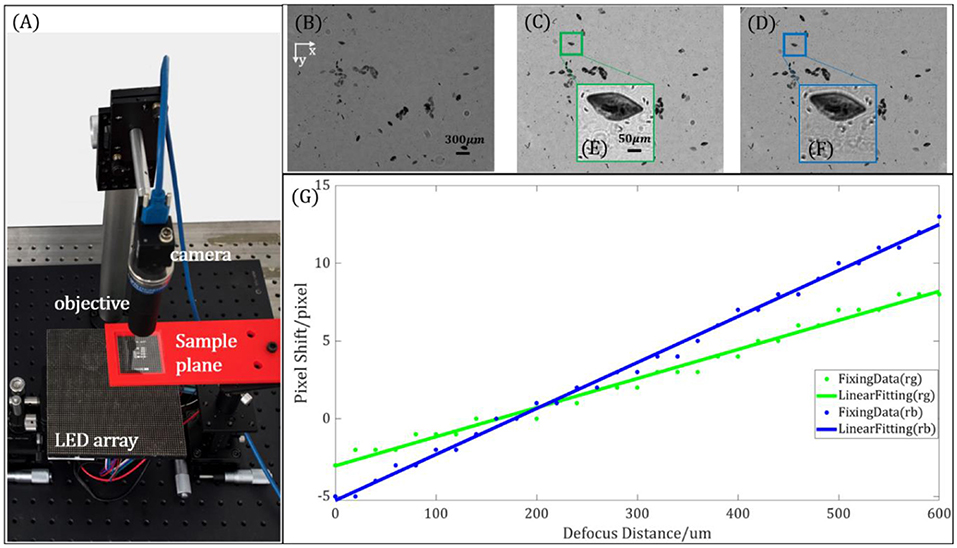
Figure 11. Scale factor calibration results. (A) System setup of the proposed method. (B–D) Through-focus images corresponding to the red, green, and blue channels, respectively; (B) is the reference image for the sum of absolute differences (SAD) image matching. (E) Window block from the green channel used for SAD image matching. (F) Window block from the blue channel. (G) Linear fitting results corresponding to system parameters A_rg and A_rb.

TABLE 2

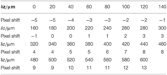
Table 2. Relationship of the defocus distance and pixel shift.

As shown in Figure 12, we use the biological sample bee wing to demonstrate the feasibility of our method. Figures 12A,B are raw data extracted from the RGB camera corresponding to the green and blue channels, respectively. By utilizing Equation (3), the defocus distances between the focus and the green/blue channel images are 256.6 and 324.6 μm, respectively. Then, as shown in Figures 12C,D, we use the AP phase retrieval approach to reconstruct both the amplitude and phase of the biological sample at the focus plane.

FIGURE 12

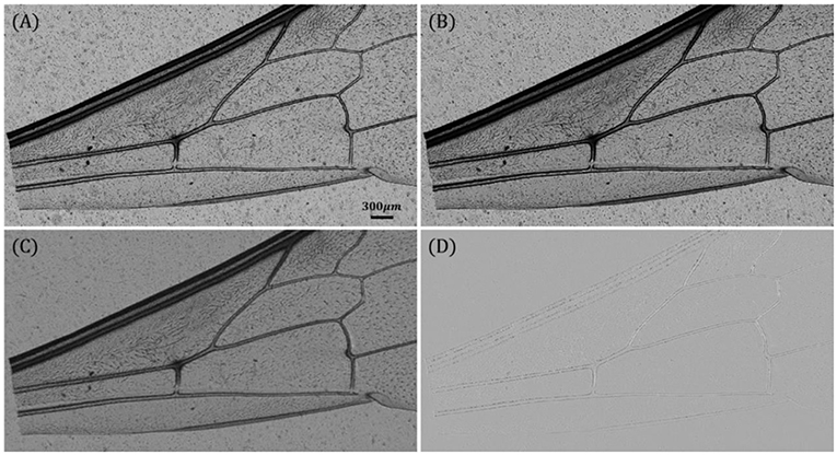
Figure 12. (A,B) Images of the green and blue channels extracted from the RGB camera. (C) Amplitude of the recovered object. (D) Phase of the recovered object.

Furthermore, similar to the simulations shown in Figure 10, we choose several defocus distances as examples to perform 3D localization. As shown in Figure 13, after obtaining the recovered object function, we propagate it onto different defocus distances (such as −200, 200, and 400 μm) with the illumination angle θ_rg. Both the amplitude and phase of the sample corresponding to the different defocus distances can be obtained by this procedure. As shown in Figures 13A–C, the enlarged red boxed sub-regions belong to the same sub-region in the amplitude of the sample while owning different defocus distances. We found that with the change of defocus distance, both the amplitude and phase of the sample will be changed. Generally speaking, Figure 13 demonstrates the feasibility of the proposed method in realizing a 3D localization in actual experiments.

FIGURE 13

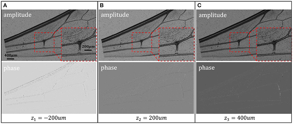
Figure 13. Three-dimensional localization results of the biological sample. (A–C) Amplitude and phase of the sample corresponding to different defocus distances.

Conclusion and Discussion

Generally speaking, through-focus intensity image acquisition methods play a critical role in AP and TIE phase retrieval approaches. In this paper, inspired by chromatic aberration of an objective and lateral shift resulting from the multi-angle illuminations of the out-of-focus sample, we proposed a single-shot through-focus intensity image acquisition strategy and realize phase recovery by the AP phase retrieval method. A Fresnel TF propagator corresponding to angle-varied illuminations is utilized in our method to solve the spectrum shift in out-of-focus imaging with oblique illuminations. Three isolated LED units are used for illumination with different wavelengths from different incident angles. Due to the chromatic aberration of an objective, there will be a lateral shift between each color channel. The red channel image is used as a reference in the calculation of the lateral shift between the red and green/blue channel images because there is no lateral shift between the defocus image and the focus image if the sample is illuminated by a normal incidence illumination. Then, the defocus distances between the focus plane and the green/blue planes can be calculated by the lateral shift between the red and green/blue channel images mathematically. Compared with the proposed methods that utilize chromatic aberration while using three normal incidence illuminations, our method can obtain the defocus distances mathematically, avoiding the requirement of accuracy measurement and complex system setup in conventional methods. Different from the time-consuming process in obtaining the correct defocus distance, our method can obtain the defocus distance quickly on the algorithm. Furthermore, an accurate focusing process is not required in the proposed method. Finally, we use some biological samples and the AP phase retrieval method to demonstrate the feasibility of the proposed method in actual experiments, and a 3D localization corresponding to different defocus distances can be realized.

Although the effectiveness of our method has been proven, there are still some details that can be improved in further works. Firstly, the calculation accuracy of the defocus distance can be increased. In our paper, we use the SAD image registration method to calculate the pixel shift between channels, whose measurement accuracy will be half of a pixel. For further work, the measurement accuracy can be increased by the method proposed in [37]. Furthermore, the sub-pixel image registration method can also be implemented to increase the measurement accuracy. Secondly, theoretically, a larger illumination angle results in a more obvious separation between two channels. However, in actual experiments, considering the effective range of the bright field in oblique illuminations, the largest tangent function between red and blue incident illumination is ${tan\theta }_{rb}=\frac{5}{90}$, which results in unobvious separations between the two channels. In further works, we can use some binary lens designed by metamaterial to obtain a more obvious chromatic aberration in experiments.

Data Availability Statement

The raw data supporting the conclusions of this article will be made available by the authors, without undue reservation.

Author Contributions

SZ conceived the idea. GZ did the experiments and writing. SZ, YH, and QH supervised the project. All the authors contributed to the review.

Funding

This work was supported by the National Natural Science Foundation of China under grants 61875012, 51735002, 61735003, and 61805011.

Conflict of Interest

The authors declare that the research was conducted in the absence of any commercial or financial relationships that could be construed as a potential conflict of interest.

References

1. Barty ANTON, Nugent KA, Paganin D, Roberts A. Quantitative optical phase microscopy. Opt Lett. (1998) 23:817–9. doi: 10.1364/OL.23.000817

CrossRef Full Text | Google Scholar

2. Choi W, Fang-Yen C, Badizadegan K, Oh S, Lue N, Dasari RR, et al. Tomographic phase microscopy. Nat Methods. (2007) 4:717–9. doi: 10.1038/nmeth1078

CrossRef Full Text | Google Scholar

3. Mann CJ, Yu L, Lo CM, Kim MK. High-resolution quantitative phase-contrast microscopy by digital holography. Opt Express. (2005) 13:8693–8. doi: 10.1364/OPEX.13.008693

PubMed Abstract | CrossRef Full Text | Google Scholar

4. Marquet P, Rappaz B, Magistretti PJ, Cuche E, Emery Y, Colomb T, et al. Digital holographic microscopy: a noninvasive contrast imaging technique allowing quantitative visualization of living cells with subwavelength axial accuracy. Opt Lett. (2005) 30:468–70. doi: 10.1364/OL.30.000468

PubMed Abstract | CrossRef Full Text | Google Scholar

5. Millerd J, Brock N, Hayes J, North-Morris M, Kimbrough B, Wyant J. Pixelated Phasemask Dynamic Interferometers. Fringe 2005. Berlin, Heidelberg: Springer (2006). p. 640–7.

Google Scholar

6. Paganin D, Nugent KA. Noninterferometric phase imaging with partially coherent light. Phys Rev Lett. (1998) 80:2586–9. doi: 10.1103/PhysRevLett.80.2586

CrossRef Full Text | Google Scholar

7. Tan Y, Wang W, Xu C, Zhang S. Laser confocal feedback tomography and nano-step height measurement. Sci Rep. (2013) 3:2971. doi: 10.1038/srep02971

PubMed Abstract | CrossRef Full Text | Google Scholar

8. Zernike F. Phase contrast, a new method for the microscopic observation of transparent objects part II. Physica. (1942) 9:974–86. doi: 10.1016/S0031-8914(42)80079-8

CrossRef Full Text | Google Scholar

9. Allen RD, David GB, Nomarski G. The Zeiss-Nomarski differential interference equipment for transmitted-light microscopy. Zeitschrift fur wissenschaftliche Mikroskopie und mikroskopische Technik. (1969)69:193–221.

PubMed Abstract | Google Scholar

10. Thibos LN. Principles of Hartmann-Shack aberrometry. J. Refractive Surg. (2000) 16:563–5. doi: 10.1364/VSIA.2000.NW6

PubMed Abstract | CrossRef Full Text | Google Scholar

11. Platt BC, Shack R. History and principles of Shack-Hartmann wavefront sensing. J Refract Surg. (2001) 17:S573–7. doi: 10.3928/1081-597X-20010901-13

PubMed Abstract | CrossRef Full Text | Google Scholar

12. Zheng G, Horstmeyer R, Yang C. Wide-field, high-resolution Fourier ptychographic microscopy. Nat Photonics. (2013) 7:739–45. doi: 10.1038/nphoton.2013.187

PubMed Abstract | CrossRef Full Text | Google Scholar

13. Zuo C, Sun J, Chen Q. Adaptive step-size strategy for noise-robust Fourier ptychographic microscopy. Opt Express. (2016) 24:20724–44. doi: 10.1364/OE.24.020724

PubMed Abstract | CrossRef Full Text | Google Scholar

14. Bian L, Suo J, Zheng G, Guo K, Chen F, Dai Q. Fourier ptychographic reconstruction using Wirtinger flow optimization. Opt Express. (2015) 23:4856–66. doi: 10.1364/OE.23.004856

PubMed Abstract | CrossRef Full Text | Google Scholar

15. Rodenburg JM, Faulkner HM. A phase retrieval algorithm for shifting illumination. Appl Phys Lett. (2004) 85:4795–7. doi: 10.1063/1.1823034

CrossRef Full Text | Google Scholar

16. Li G, Yang W, Wang H, Situ G. Image transmission through scattering media using ptychographic iterative engine. Appl Sci. (2019) 9:849. doi: 10.3390/app9050849

CrossRef Full Text | Google Scholar

17. Horstmeyer R, Chen RY, Ou X, Ames B, Tropp JA, Yang C. Solving ptychography with a convex relaxation. New J Phys. (2015) 17:053044. doi: 10.1088/1367-2630/17/5/053044

CrossRef Full Text | Google Scholar

18. Maiden AM, Humphry MJ, Zhang F, Rodenburg JM. Superresolution imaging via ptychography. J Opt Soc Am A. (2011) 28:604–12. doi: 10.1364/JOSAA.28.000604

CrossRef Full Text | Google Scholar

19. Gureyev TE, Roberts A, Nugent KA. Partially coherent fields, the transport-of-intensity equation, phase uniqueness. J Opt Soc Am A. (1995) 12:1942–6. doi: 10.1364/JOSAA.12.001942

CrossRef Full Text | Google Scholar

20. Gureyev TE, Roberts A, Nugent KA. Phase retrieval with the transport-of-intensity equation: matrix solution with use of Zernike polynomials. J Opt Soc Am A. (1995) 12:1932–41. doi: 10.1364/JOSAA.12.001932

CrossRef Full Text | Google Scholar

21. Zuo C, Chen Q, Asundi A. Boundary-artifact-free phase retrieval with the transport of intensity equation: fast solution with use of discrete cosine transform. Opt Express. (2014) 22:9220–44. doi: 10.1364/OE.22.009220

PubMed Abstract | CrossRef Full Text | Google Scholar

22. Zhang J, Chen Q, Sun J, Tian L, Zuo C. On a universal solution to the transport-of-intensity equation. Opt Lett. (2020) 45:3649–52. doi: 10.1364/OL.391823

PubMed Abstract | CrossRef Full Text | Google Scholar

23. Wittkopp JM, Khoo TC, Carney S, Pisila K, Bahreini SJ, Tubbesing K, et al. Comparative phase imaging of live cells by digital holographic microscopy and transport of intensity equation methods. Opt Express. (2020) 28:6123–33. doi: 10.1364/OE.385854

PubMed Abstract | CrossRef Full Text | Google Scholar

24. Marchesini S. Invited article: a unified evaluation of iterative projection algorithms for phase retrieval. Rev Entific Instr. (2007) 78:229–61. doi: 10.1063/1.2403783

PubMed Abstract | CrossRef Full Text | Google Scholar

25. Waller L, Kou SS, Sheppard CJ, Barbastathis G. Phase from chromatic aberrations. Opt Express. (2010) 18:22817–25. doi: 10.1364/OE.18.022817

CrossRef Full Text | Google Scholar

26. Komuro K, Nomura T. Quantitative phase imaging using transport of intensity equation with multiple bandpass filters. Appl Opt. (2016) 55:5180–6. doi: 10.1364/AO.55.005180

PubMed Abstract | CrossRef Full Text | Google Scholar

27. Kakei S, Komuro K, Nomura T. Transport-of-intensity phase imaging with polarization directed flat lenses. Appl Opt. (2020) 59:2011–5. doi: 10.1364/AO.386020

PubMed Abstract | CrossRef Full Text | Google Scholar

28. Komuro K, Saita Y, Tamada Y, Nomura T. Numerical evaluation of transport-of-intensity phase imaging with oblique illumination for refractive index tomography. In: Digital Holography and Three-Dimensional Imaging 2019, OSA Technical Digest (Optical Society of America, 2019), paper Th3A.37.

Google Scholar

29. Guo C, Bian Z, Jiang S, Murphy M, Zhu J, Wang R, et al. OpenWSI: a low-cost, high-throughput whole slide imaging system via single-frame autofocusing and open-source hardware. Opt Lett. (2020) 45:260–3. doi: 10.1364/OL.45.000260

CrossRef Full Text | Google Scholar

30. Guevorkian D, Launiainen A, Liuha P, Lappalainen V. Architectures for the sum of absolute differences operation. In: Signal Processing Systems. IEEE. (2002). p. 57–62.

Google Scholar

31. Silveira B, Paim G, Abreu B, Grellert M, Diniz CM, da Costa EA, et al. Power-efficient sum of absolute differences architecture using adder compressors. In: 2016 IEEE International Conference on Electronics, Circuits and Systems (ICECS). IEEE (2016).

Google Scholar

32. Lee W, Jung D, Ryu S, Joo C. Single-exposure quantitative phase imaging in color-coded LED microscopy. Opt Express. (2017) 25:8398. doi: 10.1364/OE.25.008398

PubMed Abstract | CrossRef Full Text | Google Scholar

33. Phillips ZF, Chen M, Waller L. Single-shot quantitative phase microscopy with color-multiplexed differential phase contrast (cDPC). PLoS ONE. (2017) 12:e0171228. doi: 10.1371/journal.pone.0171228

PubMed Abstract | CrossRef Full Text | Google Scholar

34. Netrapalli P, Jain P, Sanghavi S. Phase retrieval using alternating minimization. IEEE Trans Signal Process. (2015) 63:4814–26. doi: 10.1109/TSP.2015.2448516

CrossRef Full Text | Google Scholar

35. Fienup JR. Phase retrieval algorithms: a comparison. Appl Opt. (1982) 21:2758–69. doi: 10.1364/AO.21.002758

CrossRef Full Text | Google Scholar

36. Voelz DG. Computational Fourier Optics: A MATLAB Tutorial. Las Cruces, NM: SPIE (2011).

Google Scholar

37. Zhou G, Zhang S, Hu Y, Hao Q. Single-shot sequential projection phase retrieval and 3D localization from chromatic aberration. Opt Express. (2020) 28:9976–87. doi: 10.1364/OE.389260

PubMed Abstract | CrossRef Full Text | Google Scholar