Mean First-Passage Time on Scale-Free Networks Based on Rectangle Operation

1. Introduction

In the past several decades, some delightful properties related to complex networks have been obtained. For example, Watts and Strogatz discovered and explained the ubiquitous small-world property of real social networks by building small-world network models with a relatively small diameter [1]; Barabasi and Albert constructed a scale-free network model to reveal the fact that degree distribution obeys the power-law distribution in real networks [2, 3]. These two classical works have inspired many scholars to devote themselves to researching about complex networks, especially random walks in complex networks [4–9].

The random walks on complex networks was of typical interest in various kinds of scientific fields, such as statistics physics, combinatorial mathematics, computer science, chemistry, social and economic science as well as biological science [10–14]. Random walks were not merely an effective instrument to solve various problems, and have found diverse applications in real-world networks, for example, routing [15], searching [16], sampling [17] and data collection [18, 19], community detection [20, 21], network synchronization [22, 23], random algorithm [24, 25], and so on [26–28].

In this paper, we define a graphic operation to generate a network, then we discuss the topological structure of our networks, such as degree distribution, clustering coefficient, diameter, as we will shortly explain. After that, we investigate the relationship among adjacency matrix, diagonal matrix, and Lapalican matrix. In addition, we investigate random walks on scale-free networks, with a goal to determine solution of mean first-passage time. Besides, by taking full advantage of the relationship between the first-passage time and effective resistance, we induce explicit formulas of mean first-passage time which scales linearly with the network size. Our work provides the relationship between mean first-passage time and network size.

The following content of this paper will be divided into the subsequent three parts. In section 2, we introduce several relative concepts for graphs, electrical networks, and random walks. After that, in section 3, we provide the network construction process about generating scale-free network and discuss its topological properties in further. In addition, we present the result for mean first-passage time on our scale-free networks. Finally, we draw a brief conclusion and put forward some unresolved issues for next step in section 4.

2. Preliminaries

In this section, we will introduce several fundamental concepts for graphs, electrical networks, and random walks. These basic concepts are closely related to our work in the coming subsections.

2.1. Several Concepts

A graph is a structure described in a set of objects, some of which are “related” in a certain sense. These objects correspond to mathematical abstractions called vertices (also called nodes), and each related pair of vertices is called an edge (also called link). Generally, a graph is depicted graphically as a set of vertices, connected by lines or curves along the edges. In graph theory, a graph is denoted as G = (ν, ε), and notations N = |ν| and E = |ε| are the vertex number and edge number of G, where ν and ε are vertex set and edge set of G, respectively. The sum of the degree of all vertices in G is 2E, and the average degree of a graph is the average value of all vertex degrees over the entire graph, denoted by 2E/N. The R-graph is the graph by creating a new vertex corresponding to each edge of G and by adding edges between each created vertex and corresponding edge's end vertices, the graph R(G) appeared in [29]. Here, all graphs are simple undirected connected graphs, namely, no loops and no multiple edge connecting the same couple of vertices. In this paper, there is no need to distinguish between graph and network, because graphs are abstract representations of networks. The meaning of these two terms is considered to be the same.

We use the labels 1, 2, 3, ⋯, N, to represent the N vertices in graph G. For a graph, it can be denoted by two different matrices, namely, adjacency matrix and Laplacian matrix. Notice that, the adjacency matrix A_G = (a_ij)_N×N is defined to be the N × N constant matrix those ijth entry is 1 if vertex i and vertex j are connected by an edge, 0 is otherwise. We use the symbol ${N}(i)=\{x|(x,i)\in \epsilon \}$ to represent the set of neighbors of vertex i in G, hence, the degree of vertex i is the number of edges of G incident with i, can be regarded as $d_i=\left|{N}(i)\right|$. The diagonal matrix, denoted by D_G, may be defined as follows: the ith diagonal entry is d_i, while all non-diagonal entries are zero. It has to be remarked that the corresponding Laplacian matrix of G can be referred to as L_G = D_G − A_G. Let λ₁, λ₂, ⋯, λ_N stand for the N eigenvalues of Laplacian matrix L_G, which can be rearranged in an non-decreasing order as follows, 0 = λ₁ ≤ λ₂ ≤ ⋯ ≤ λ_N. From above description, it can be said with certainty that all eigenvalues are non-negative for G. The other standard graph theoretic notations we used of our networks are mainly followed [30].

2.2. Electrical Networks

Before continuing, we firstly pay attention to the following several results concerning effective networks that we need in the proofs. A graph can be viewed as an electrical network by replacing each edge of G with a unit resistance. Therefore, we also apply the G = (ν, ε) to stand for corresponding electrical networks generated by G. Now we have to introduce some notations about electrical networks. The effective resistance between any two vertices i and j, denoted by Ω_ij, is defined as the potential difference between i and j when the unit current is remained from i to j. If i = j, Ω_ij is equal to zero.

It is generally recognized that effective resistances of the network are well-defined, which can be regarded as a measure of distance. There are a number of scholars devoted their effort to investigating the properties of effective resistance and discovering fruitful results.

Lemma 2.1. (Foster's [31]) The sum of effective resistances along the edges of a connected graph G is equal to N − 1, namely

$\begin{array}{ll}{\displaystyle \sum _{\begin{array}{c}i<j\\ (i,j)\in \epsilon \end{array}}}{\Omega }_{ij}=N-1& (1)\end{array}$

In [32, 33], Chen et al. prove the effective resistance local sum rules by applying the inseparable relations between random walks and electrical network, which can be described by the following lemma.

Lemma 2.2. For an electrical network G = (ν, ε), any couple of vertices i, j (i ≠ j) belongs to ν, we have

$\begin{array}{ll}{d}_i{\Omega }_{ij}+{\displaystyle \sum _{k\in {N}(i)}}({\Omega }_{ik}-{\Omega }_{jk})=2& (2)\end{array}$

The effective resistance has been defined and discussed in [34], also referred to as, Kirchhoff index K(G). So, one arrives at the Kirchhoff index as follows

$\begin{array}{ll}K(G)={\displaystyle \sum _{\begin{array}{c}i\in \nu ,\\ j\in \nu \end{array}}}{\Omega }_{ij}& (3)\end{array}$

Lately, one finds Kirchhoff index of a graph G is closely related to the Laplacian eigenvalue and is expressed in term of eigenvalues in [35]

$\begin{array}{ll}K(G)=N{\displaystyle \sum _{i=2}^N}\frac{1}{{\lambda }_i}& (4)\end{array}$

Based on the Kirchhoff index, we now put forth on another metrics, the average effective resistance over all vertex pairs in G, that is,

$\begin{array}{ll}\overline{K}(G)=\frac{K(G)}{N(N-1)}=\frac{1}{N-1}{\displaystyle \sum _{\begin{array}{c}i=2\end{array}}^N}\frac{1}{{\lambda }_i}& (5)\end{array}$

which can be applied to measure the network robustness and stability of G: the smaller the value $\overline{K}(G)$, the more robust the network is. In [36], Liu discuss several results of resistance distance and Kirchhoff index of subdivision vertex edge corona for graphs. In [37, 38], Liu et al. explore some results of resistance distance and Kirchoff index by virture of R-graphs.

In what follows, we will demonstrate these metrics to define random walks through rigorous mathematical analysis.

2.3. Random Walks

We can define an unbiased, discrete time random walk on a certain connected graph G = (ν, ε). Given a graph G and an initial vertex, at each time step, the walker goes to a certain neighbor of the vertex with equal probability from its current location. The essence of stochastic process is the Markov process [39], described by the transition matrix T = D⁻¹A, with the ijth element being a_ij/d_i that stands for the probability of moving to j from i in one time step. When G is finite, connected, and then the random walk is ergodic if there is a unique stationary distribution $\pi ={({\pi }_1,{\pi }_2\cdots ,{\pi }_N)}^{\top }$ meeting the following requirements: ${\pi }_i=d_i/(2E),\sum _{i=1}^N{\pi }_i=1,{\pi }^{\top }T={\pi }^{\top }$.

A crucial quantity pertaining to random walks is first-passage time, also known as hitting time. The first-passage time from a given site i to destination j, denoted by F_ij, is the expected time for a walker starting from source vertex i to first reach the destination vertex j. It has to be noticed that F_ij ≠ F_ji in some situations. With regarded to first-passage time, the commute time C_ij starts from i to j, then goes back, denoted by C_ij = F_ij + F_ji, is symmetric. We can discover the fact that the relationship between commute time and first-passage time.

Lemma 2.3. The communte time C_ij between any pair of vertices i and j(i ≠ j) has a relationship with the effective resistance, so we have

$\begin{array}{ll}{C}_{ij}=2E{\Omega }_{ij}& (6)\end{array}$

The mean first-passage time $\overline{F}(G)$ of a network is the average value of first-passage times over all vertex pairs, namely

$\begin{array}{ll}\overline{F}(G)=\frac{1}{N(N-1)}{\displaystyle \sum _{\begin{array}{c}i\ne j\end{array}}^N}{\displaystyle \sum _{j=1}^N}{F}_{ij}& (7)\end{array}$

As is the simple particular case, the mean first-passage time can be determined exactly. For example, it is generally recognized that the mean first-passage time for the complete graph with N vertices is N − 1. It indicates that the mean first-passage time of complete graph scales linearly with N.

However, due to the high density of the complete graph, it is impossible to extend to real networks, most of which are sparse with the average degree tends to a fixed constant [40, 41], and also display scale-free properties [42, 43].

Combining with above discussions, the mean first-passage time of a network G can be represented as the expression related to the eigenvalues of its Laplacian matrix.

Lemma 2.4. The mean first-passage time $\overline{F}(G)$ has a relationship with the eigenvalues of Laplacian matrix of G, so we have

$\begin{array}{ll}\overline{F}(G)=\frac{EK(G)}{N(N-1)}=\frac{2E}{N-1}{\displaystyle \sum _{i=2}^N}\frac{1}{{\lambda }_i}& (8)\end{array}$

Taking full advantage of above statement, let us turn our sight into calculating mean first-passage time $\overline{F}(S_t)$ of our scale-free networks.

3. Mean First-Passage Time of Scale-Free Networks

In this section, we study the mean first-passage time of our network with remarkable scale-free property. To this end, firstly, we introduce rectangle operation in graphic operation to generate a class of scale-free networks and discuss the topological properties of our networks. Then, we illustrate three matrices of our network, including, Laplacian matrix, diagonal matrix, and adjacent matrix; and derive the relationship among them. In addition, to evaluate the mean effective resistance of our network, we show the effective resistance between any two vertices in our networks. Finally, for our networks, we calculate the mean first-passage time and prove that mean first-passage time is linearly proportional to the number of vertices. In what follows, we will present critical constituents in the coming subsections.

3.1. Network Construction and Topological Properties

Before proceeding, we have to introduce a graphic operation, referred to as rectangle operation in this paper, which is explained in more detail, as follows

3.1.1. Rectangle Operation

For a certain edge uv with two end-vertices u and v, we create an edge xy with two end-vertices x and y, and attach the vertices u to x and v to y using two new edges, respectively. Then, we generate a cycle C₄. Such an operation process is called a rectangle operation. Figure 1 gives the rectangle operation process.

FIGURE 1

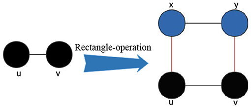
Figure 1. The illustration of graph operation, rectangle operation, where each edge is formed a cycle on right-hand of arrow, where blue vertices represent new vertices.

Taking useful advantage of rectangle operation, let us turn our attention to constructing our networks S_t, which has been discussed in [40]. Let S_t = (ν_t, ε_t) represent the network after t time steps. Then the networks are constructed in the following process: at t = 0, the initial network S₀ is a graph in which two vertices are attached to an edge. At t ≥ 1, S_t is created from S_t−1 by conducting the rectangle operation for each edge of network S_t−1. The generation process is repeated t times to obtain S_t from S₀. Figure 2 shows three networks with time step t = 0, t = 1, t = 2, respectively. Besides, we also give the Construction Pseudo-code to describe the network generation process in Algorithm 1. The time complexity of the Algorithm 1 depends on time t and the number of edges of S_t.

FIGURE 2

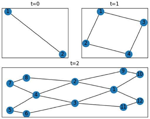
Figure 2. The illustration of the network generation process when the time step is t = 0, 1, 2, respectively.

ALGORITHM 1

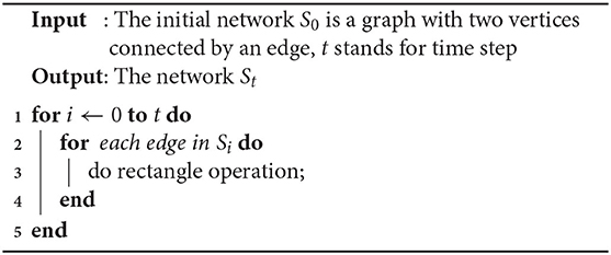
Algorithm 1. Construction Pseudo-code

Now we calculate several fundamental quantities, for example, the number of all vertices and edges in S_t. Let N_t = |ν_t| and E_t = |ε_t| be the vertex number and edge number of S_t, where ν_t and ε_t are vertex set and edge set of S_t. For S_t, let ${{W}}_t={\nu }_t\backslash {\nu }_{t-1}$ and $W_t=\left|{{W}}_t\right|$ represent the set of new vertices created at time step t and the number of these vertices, respectively. Together with the construction process, it is not difficult to obtain E_t = 4E_t−1, W_t = 2E_t−1, and N_t = N_t−1 + W_t−1 = N_t−1 + 2E_t−1. Due to N₀ = 2, E₀ = 1, we can easily obtain the following the expressions $E_t=4^t$, $W_t=2·4^{t-1}$, and $N_t=\frac{2}{3}(4^t+2)$ hold for all t ≥ 0. By the definition of average degree, we have $\langle k\rangle =\frac{2E_t}{N_t}$, which tends to 3 for large time step t. It has to be noticed that the network with identical average degree has been explored in [42].

Besides, armed with the definition of sparsity, we call a network is sparse if $E_t\ll \frac{N_t(N_t-1)}{2}$, namely, the value is close to a constant, which is obtained by the number of edges divides the number of vertices. So, we assert that the resulting network S_t is sparse network. Let $d_i^{(t)}$ indicate the number of edges connected to vertex i in S_t, which is created at iterations t_i(t_i ≥ 0). Then for any vertex i, its degree satisfies the following expression $d_i^{(t)}=2d_i^{(t-1)}$.

By virture of generation process of networks aforementioned, it goes without saying that the degree spectrum of our networks is a series of discrete positive integers. Armed with probability theory, it has to be noticed that the degree distribution exhibits a unique power-law distribution P(k) ~ k^−γ with a constant value γ = 3, where P(k) is the probability that a randomly selected vertex is with degree k. It is clearly recognized that the same exponent has been studied in other references, for instance, [41, 42], to name but a few. What is noteworthy is that both sparsity and scale-free property can normally be found in many complex networks, such as [2, 28, 40–42]. In addition, it is easily to note that our network is not a homogeneous network, because the degree distribution obeys the power-law distribution, and there are few nodes with larger degrees in our network, it is a heterogeneous network.

Moreover, for the sake of understanding the behavior of network, we have to turn attention to the clustering coefficient. The clustering coefficient c_i of vertex i is a measure of the number of edges “around” the vertex i. c_i is given by the average fraction of pairs of neighbors of the same vertex that are also neighbors of each other, i.e., c_i = 2E_i/[k_i(k_i − 1)], where E_i represents the number of actual edges between the vertex neighbors. Since our rectangle operation always obtain a cycle C₄. At time step t, it can be said with certainty that the clustering coefficient of every vertex in S_t is 0, namely, we have c_i = 0 for every vertex. Thus, we get the result that clustering coefficient of entire network is also zero. It can be noted that the same clustering coefficient has been obtained in the networks [40, 42].

In addition, network diameter is an important index to measure the size of the network. It is defined as the maximum distance between any two vertices in the network, where the distance refers to the length of the shortest path. We may find that diameter Dia(S_t) is approximately equal to ln N_t, directly showing Dia(S_t) is a relatively small. Evidently, the diameter increases logarithmically withof the number of vertices. The diameter of our network has been thoroughly investigated in [40, 42].

3.2. Relations Between Matrices

We use the notation A_t represent the adjacency matrix of S_t. A_t(i, j) is an element of the adjacency matrix at row i and column j of A_t, A_t(i, j) = 1 if there exists an edge connecting vertices i and j in S_t, A_t(i, j) = 0 otherwise. We regard the diagonal degree matrix of S_t as the notation D_t, with the ith diagonal is denoted by $d_i^{(t)}$, the degree of vertex i. Then, let L_t = D_t − A_t stand for Laplacian matrix L_t of S_t. Next, we will deduce the recursive relationship among A_t, D_t, and L_t.

For network S_t, the notations α and β are the set of old vertices that are all vertices in S_t−1 and the set of new vertices in ${{W}}_t$, respectively. Then, we represent A_t with block form as follows

$\begin{array}{ll}{A}_t=\left(\begin{array}{cc}{A}_t^{\alpha ,\alpha }& A_t^{\alpha ,\beta }\\ A_t^{\beta ,\alpha }& A_t^{\beta ,\beta }\end{array}\right)=\left(\begin{array}{cc}{A}_{t-1}& A_t^{\alpha ,\beta }\\ A_t^{\beta ,\alpha }& 0\end{array}\right)& (9)\end{array}$

where $A_t^{\alpha ,\alpha }=A_{t-1}$, $A_t^{\beta ,\beta }$ is equal to zero matrix with order W_t × W_t, and $A_t^{\alpha ,\beta }={(A_t^{\beta ,\alpha })}^{\top }$ which are obvious according to construction process.

Let I stand for the identity matrix. After that, the diagonal matrix D_t holds

$\begin{array}{ll}{D}_t=\left(\begin{array}{cc}{D}_t^{\alpha ,\alpha }& 0\\ 0& D_t^{\beta ,\beta }\end{array}\right)=\left(\begin{array}{cc}2D_{t-1}& 0\\ 0& 2I\end{array}\right)& (10)\end{array}$

which is based on the result that during the recursive procedure of network construction from time step t − 1 to time step t, the degree of each vertex in set α is increased by 2 times, yet the degree of all vertices in set β is 2. Hence, it goes without saying that the Laplacian matrix L_t can be written as

$\begin{array}{ll}{L}_t=D_t-A_t=\left(\begin{array}{cc}2D_{t-1}-A_{t-1}& -A_{t-1}^{\alpha ,\beta }\\ -A_{t-1}^{\beta ,\alpha }& 2I\end{array}\right)& (11)\end{array}$

According to above analysis, we have completed the recursive relations among A_t, D_t, and L_t.

3.3. Relations Between Effective Resistances

As stated in the previous paragraph, the mean first-passage time of a certain connected graph is related to its effective resistance. To calculate the mean effective resistance of scale-free networks, what calls for special attention is the iterative process of effective resistance for any pair of old vertices.

Before continuting further, we attempt to introduce some concepts of {1}-inverse of a matrix. Matrix M is said to be a inverse of X if M satisfies XMX = X. Let X^† represent one of the {1}-inverses of X. We present a result associated with the {1}-inverse of the block matrix.

Lemma 3.1. For a block matrix $X=\left(\begin{array}{cc}A& B\\ B^T& C\end{array}\right)$, where the determinant of C is not equal to zero, if there exists a {1}-inverse R^† for R = A − BC⁻¹B^⊤, we have

$\begin{array}{ll}{X}^{†}=\left(\begin{array}{cc}{R}^{†}& -R^{†}B{C}^{-1}\\ -C^{-1}{B}^T{R}^{†}& C^{-1}{B}^T{R}^{†}B{C}^{-1}+C^{-1}\end{array}\right)& (12)\end{array}$

which is a {1}-inverse of X.

Proof: In order to verify the fact that X has a {1}-inverse, it is sufficient to illustrate that there exists three matrixes P, Q, Y with appropriate order meets PXQ = Y, where P and Q are non-singular, and Y has a {1}-inverse. There is no doubt that we can account for as follows. If the above conditions are holded, we may as well find a matrix X^† = QY^†P. It may be safely said that XX^†X − X = 0, which indicates that X^† = QY^†P is a {1}-inverse of X. Consequently, we turned the issue of solving a {1}-inverse of X into solving matrices P, Q, and Y.

Let $P=\left(\begin{array}{cc}I& -B{C}^{-1}\\ 0& I\end{array}\right)$, $Q=\left(\begin{array}{cc}I& 0\\ -C^{-1}{B}^T& I\end{array}\right)$, and $Y=\left(\begin{array}{cc}R& 0\\ 0& C\end{array}\right)$. Together with known condition, namely, P and Q are invertible, Y has a {1}-inverse, and PXQ = Y. Thus,

$\begin{array}{ll}\begin{array}{l}{X}^{†}=\left(\begin{array}{cc}I& 0\\ -C^{-1}{B}^T& I\end{array}\right)\left(\begin{array}{cc}{R}^{†}& 0\\ 0& C^{-1}\end{array}\right)\left(\begin{array}{cc}I& B{C}^{-1}\\ 0& I\end{array}\right)\\ =\left(\begin{array}{cc}{R}^{†}& -R^{†}B{C}^{-1}\\ -C^{-1}{B}^T{R}^{†}& -C^{-1}{B}^T{R}^{†}B{C}^{-1}+C^{-1}\end{array}\right)\end{array}& (13)\end{array}$

Hence, we complete the proof of Lemma 3.1.□

Lemma 3.2. Let $L_{ij}^{†}$ represent the (i, j)th entry of any {1}-inverse L^† of its Laplacian matrix L. Then, for any pairs of vertices i, j ∈ ν, the effective resistance Ω_ij is given by

$\begin{array}{ll}{\Omega }_{ij}=L_{ii}^{†}+L_{jj}^{†}-L_{ij}^{†}-L_{ji}^{†}& (14)\end{array}$

Lemma 3.3. For our scale-free networks S_t after t time steps, we have

$\begin{array}{ll}{A}_t^{\alpha ,\beta }{A}_t^{\beta ,\alpha }=2\left(D_{t-1}+A_{t-1}\right)& (15)\end{array}$

Proof: In order to prove $A_t^{\alpha ,\beta }{A}_t^{\beta ,\alpha }=2\left(D_{t-1}+A_{t-1}\right)$, it is necessary to prove that the corresponding elements in the two matrices are the same. Let Q_t = 2(D_t + A_t), the elements of which are: $Q_t\left(i,j\right)=2d_i^{\left(t\right)}$ if i = j and Q_t(i, j) = 2A_t(i, j) otherwise. Let $Z_{t-1}=A_t^{\alpha ,\beta }{A}_t^{\beta ,\alpha }$. Below we verify that the elements Z_t−1(i, j) of Z_t is equal to the element of Q_t.

It has to be noticed that matrix $A_t^{\beta ,\alpha }$ can be divided into N_t−1 column vectors $x_i={\left(x_{i,N_{t-1}+1},x_{i,N_{t-1}+2}\cdots ,x_{i,N_t}\right)}^{\top }\left(i=1,2,\cdots ,N_{t-1}\right)$ as

$\begin{array}{l}{A}_t^{\beta ,\alpha }=(x_1,x_2,\cdots ,x_{N_{t-1}})\end{array}$

where let x_i represent the connection between the vertex i ∈ α and all vertices belongs to β. From $A_t^{\alpha ,\beta }={\left(A_t^{\beta ,\alpha }\right)}^{\top }$, one has $A_t^{\alpha ,\beta }={\left(x_1,x_2,\cdots ,x_{N_{t-1}}\right)}^{\top }$. Thus,

$\begin{array}{ll}\begin{array}{l}{A}_t^{\alpha ,\beta }{A}_t^{\beta ,\alpha }={(x_1,x_2,\cdots ,x_{N_{t-1}})}^{\top }(x_1,x_2,\cdots ,x_{N_{t-1}})\\ ={(x_i^{\top }{x}_j)}_{N_{t-1}\times N_{t-1}}\end{array}& (16)\end{array}$

according to which the elements Z_t−1(i, j) of $A_t^{\alpha ,\beta }{A}_t^{\beta ,\alpha }$ can be discussed by dividing two different cases, namely, i = j and i ≠ j.

When i = j, the diagonal element of Z_t−1 is $Z_{t-1}\left(i,i\right)=x_i^{\top }{x}_i$, i.e., the number of all new created vertices in β that are connected with vertex i. Henceforth, $Z_{t-1}\left(i,i\right)=d_i^{\left(t\right)}-d_i^{\left(t-1\right)}=2d_i^{\left(t-1\right)}=Q_{t-1}\left(i,i\right)$.

When i ≠ j, the non-diagonal element of matrix Z_t−1 can be expressed as

$\begin{array}{ll}\begin{array}{l}{Z}_{t-1}\left(i,j\right)=x_i^{\top }{x}_j={\displaystyle \sum _{k\in \beta }}\left(x_{i,k}·x_{j,k}\right)\\ ={\displaystyle \sum _{k\in \beta }}\left(A_t\left(i,k\right)\right)\left(A_t\left(j,k\right)\right)\\ ={\displaystyle \sum _{\begin{array}{c}{A}_t\left(i,k\right)=1\\ A_t\left(j,k\right)=1\end{array}}}{A}_t\left(i,j\right)\\ =2A_{t-1}\left(i,j\right)=Q_{t-1}\left(i,j\right)\end{array}& (17)\end{array}$

here we apply the construction rule, that is, each edge in S_t−1 produces 2 new vertices at time steps t.

This completes the proof of Lemma 3.3.□

We use the notations ${\Omega }_{ij}^{\left(t\right)}$ and L^† to represent the effective resistance for any couple of vertices i and j and the {1}-inverse of Laplacian matrix L_t of S_t, respectively.

Lemma 3.4. Let i, j ∈ ν_t−1 be a couple of old vertices in S_t. Then, ${\Omega }_{ij}^{\left(t-1\right)}$ follows the relation

$\begin{array}{ll}{\Omega }_{ij}^{\left(t\right)}=\frac{1}{2}{\Omega }_{ij}^{\left(t-1\right)}& (18)\end{array}$

Proof: Arbitrary {1}-inverse $L_t^{†}$ of Laplacian matrix L_t is expressed by

$\begin{array}{ll}{L}_t^{†}=\left(\begin{array}{cc}{L}_{\alpha ,\alpha }^{†}& L_{\alpha ,\beta }^{†}\\ L_{\beta ,\alpha }^{†}& L_{\beta ,\beta }^{†}\end{array}\right)& (19)\end{array}$

By Equation (11) and Lemma 3.1 and Lemma 3.3,

$\begin{array}{ll}\begin{array}{l}{L}_{\alpha ,\alpha }^{†}={\left(2D_{t-1}-A_{t-1}-(-A_{t-1}^{\alpha ,\beta }){(2I)}^{-1}(-A_{t-1}^{\beta ,\alpha })\right)}^{†}\\ ={\left(2D_{t-1}-A_{t-1}-\frac{1}{2}\times 2\left(D_{t-1}+A_{t-1}\right)\right)}^{†}\\ =L_{t-1}^{†}\end{array}& (20)\end{array}$

By Lemma 3.2 and Equation (20), for i, j ∈ ν_t−1,

$\begin{array}{ll}\begin{array}{l}{\Omega }_{ij}^{\left(t\right)}\\ =L_{\alpha ,\alpha }^{†}\left(i,i\right)+L_{\alpha ,\alpha }^{†}\left(j,j\right)-L_{\alpha ,\alpha }^{†}\left(i,j\right)-L_{\alpha ,\alpha }^{†}\left(j,i\right)\\ =\frac{1}{2}\left(L_{t-1}^{†}\left(i,i\right)+L_{t-1}^{†}\left(j,j\right)-L_{t-1}^{†}\left(i,j\right)-L_{t-1}^{†}\left(j,i\right)\right)\\ =\frac{1}{2}{\Omega }_{ij}^{\left(t-1\right)}\end{array}& (21)\end{array}$

which provides the recursive process for effective resistance between any pair of old vertices in S_t.□

In the following, we will display that the effective resistance between arbitrary two vertices in S_t can be expressed by effective resistance of the pair of vertices in S_t−1. Because Lemma 3.4 provides the recursive rule of effective resistance between any pairs of vertices in S_t−1, we merely like to believe that the effective resistance between any two vertices in S_t can be expressed by pairs of vertices in S_t−1. To achieve our objective, we first define several other parameters. For arbitrary two subsets X and Y belongs to ν_t−1 in S_t−1, we define

${\Omega }_{X,Y}^{\left(t-1\right)}={\displaystyle \sum _{i\in X,j\in Y}}{\Omega }_{ij}^{\left(t-1\right)}$

For a vertex $i\in {{W}}_t$ in S_t, we use Δ_i = {p, q} to denote the set of neighbors of i. Apparently, p, q ∈ ν_t−1. Then, we define

${\Omega }_{{\Delta }_i}^{\left(t\right)}={\Omega }_{pq}^{\left(t\right)}$

Lemma 3.5. For t ≥ 0, $i\in {{W}}_t$,

$\begin{array}{ll}{\Omega }_{i,{\Delta }_i}^{\left(t\right)}=1+\frac{1}{2}{\Omega }_{{\Delta }_i}^{\left(t\right)}& (22)\end{array}$

Proof: According to Lemma 2.2, for every $i\in {{W}}_t$, combined with the neighbor vertex set Δ_i = {p, q}, we have

$\begin{array}{l}2{\Omega }_{ip}^{\left(t\right)}+{\Omega }_{i,{\Delta }_i}^{\left(t\right)}-{\Omega }_{p,{\Delta }_i}^{\left(t\right)}=2\end{array}$

and

$\begin{array}{l}2{\Omega }_{iq}^{\left(t\right)}+{\Omega }_{i,{\Delta }_i}^{\left(t\right)}-{\Omega }_{q,{\Delta }_i}^{\left(t\right)}=2\end{array}$

summing the above two equations gives

$\begin{array}{l}2{\Omega }_{i,{\Delta }_i}^{\left(t\right)}+2{\Omega }_{i,{\Delta }_i}^{\left(t\right)}-{\Omega }_{{\Delta }_i,{\Delta }_i}^{\left(t\right)}=4\end{array}$

that is,

$\begin{array}{l}{\Omega }_{i,{\Delta }_i}^{\left(t\right)}=1+\frac{1}{4}{\Omega }_{{\Delta }_i,{\Delta }_i}^{\left(t\right)}=1+\frac{1}{2}{\Omega }_{{\Delta }_i}^{\left(t\right)}\end{array}$

as desired.□

Lemma 3.6. For t ≥ 0, $i\in {{W}}_t,j\in {{W}}_{t-1}$,

$\begin{array}{ll}{\Omega }_{ij}^{\left(t\right)}=\frac{1}{2}\left(1-\frac{1}{2}{\Omega }_{{\Delta }_i}^{\left(t\right)}+{\Omega }_{i,j}^{\left(t\right)}\right)& (23)\end{array}$

Proof: For $i\in {{W}}_t,j\in {{W}}_{t-1}$, By Lemma 2.2

$d_i^{\left(t\right)}{\Omega }_{ij}^{\left(t\right)}+{\Omega }_{{\Delta }_i,i}^{\left(t\right)}-{\Omega }_{{\Delta }_i,j}^{\left(t\right)}=2$

Providing $d_i^t=2$ and applying Lemma 3.5, it follows that

$\begin{array}{l}\begin{array}{l}{\Omega }_{ij}^{\left(t\right)}=\frac{1}{2}\left(2-{\Omega }_{{\Delta }_i,i}^{\left(t\right)}+{\Omega }_{{\Delta }_i,j}^{\left(t\right)}\right)\\ =\frac{1}{2}\left(1+{\Omega }_{{\Delta }_i,j}^{\left(t\right)}-\frac{1}{2}{\Omega }_{{\Delta }_i}^{\left(t\right)}\right)\end{array}\end{array}$

we complete the proof.□

Lemma 3.7. For t ≥ 0, $i,j\in {{W}}_t,i\ne j$,

$\begin{array}{ll}{\Omega }_{ij}^{\left(t\right)}=1-\frac{1}{4}\left({\Omega }_{{\Delta }_i}^{\left(t\right)}+{\Omega }_{{\Delta }_j}^{\left(t\right)}\right)+\frac{1}{4}{\Omega }_{{\Delta }_i,{\Delta }_j}^{\left(t\right)}& (24)\end{array}$

Proof: For a pair of different vertices i and j in ${{W}}_t$, armed with Lemma 2.2

$d_i^{\left(t\right)}{\Omega }_{ij}^{\left(t\right)}+{\Omega }_{{\Delta }_i,i}^{\left(t\right)}-{\Omega }_{{\Delta }_i,j}^{\left(t\right)}=2$

considering $d_i^t=2$ and using Lemma 3.5 and Lemma 3.6,

$\begin{array}{l}\begin{array}{l}{\Omega }_{ij}^{\left(t\right)}=\frac{1}{2}\left(2-{\Omega }_{{\Delta }_i,i}^{\left(t\right)}+{\Omega }_{{\Delta }_i,j}^{\left(t\right)}\right)\\ =\frac{1}{2}\left(2-{\Omega }_{{\Delta }_i,i}^{\left(t\right)}+{\displaystyle \sum _{k\in {\Delta }_i}}{\Omega }_{j,k}^{\left(t\right)}\right)\\ =\frac{1}{2}\left(2-{\Omega }_{{\Delta }_i,i}^{\left(t\right)}+{\displaystyle \sum _{k\in {\Delta }_i}}\frac{1}{2}\left(1-\frac{1}{2}{\Omega }_{{\Delta }_j}^{\left(t\right)}+{\Omega }_{{\Delta }_j,k}^{\left(t\right)}\right)\right)\\ =\frac{1}{2}\left(1-\frac{1}{2}{\Omega }_{{\Delta }_i}^{\left(t\right)}+\left(1-\frac{1}{2}{\Omega }_{{\Delta }_j}^{\left(t\right)}+\frac{1}{2}{\Omega }_{{\Delta }_i,{\Delta }_j}^{\left(t\right)}\right)\right)\\ =1-\frac{1}{4}\left({\Omega }_{{\Delta }_i}^{\left(t\right)}+{\Omega }_{{\Delta }_j}^{\left(t\right)}\right)+\frac{1}{4}{\Omega }_{{\Delta }_i,{\Delta }_i}^{\left(t\right)}\end{array}\end{array}$

Thus we complete the proof.□

3.4. Mean First-Passage Time

Our next task is to discuss the mean first-passage time for our scale-free networks S_t, by applying the relationship between first-passage time and average effective resistance. To achieve our task, we present several parameters in following descriptions. For the two subsets X and Y of set of vertices ν_t in S_t, we have

$\begin{array}{l}{K}_{X,Y}={\displaystyle \sum _{i\in X,j\in Y}}{\Omega }_{ij}^{\left(t\right)}\end{array}$

where K_{X, Y} is the Kirchhoff index of S_t, for the sake of obtaining this result, we give the following results.

Lemma 3.8. For t ≥ 0,

$\begin{array}{ll}{\displaystyle \sum _{i\in {{W}}_t}}{\Omega }_{{\Delta }_i}^{\left(t\right)}=\frac{\left(N_{t-1}-1\right)}{2}& (25)\end{array}$

Proof: It has to be noted that each edge of S_t−1 produces exactly two new vertices of S_t, summing ${\Omega }_{{\Delta }_i}^{t-1}$ over Δ_i of all new vertices i ∈ W_t in S_t is equal to summing ${\Omega }_{x,y}^t$ times over all edges (x, y) in S_t−1. Then, on the basis of Lemma 2.1, we have

$\begin{array}{l}\begin{array}{l}{\displaystyle \sum _{i\in {{W}}_t}}{\Omega }_{{\Delta }_i}^{\left(t\right)}=2{\displaystyle \sum _{\left(x,y\right)\in {\epsilon }_{t-1}}}{\Omega }_{x,y}^{\left(t\right)}\\ =2{\displaystyle \sum _{\left(x,y\right)\in {\epsilon }_t}}\frac{1}{2}{\Omega }_{x,y}^{\left(t-1\right)}\\ =\frac{\left(N_{t-1}-1\right)}{2}\end{array}\end{array}$

we have done.□

Lemma 3.9. For t ≥ 0, and Y ⊂ ν_t−1

$\begin{array}{ll}{\displaystyle \sum _{i\in {{W}}_t}}{\Omega }_{{\Delta }_i,Y}^{\left(t\right)}={\displaystyle \sum _{x\in {\nu }_{t-1}}}{d}_x^{\left(t-1\right)}{\Omega }_{x,Y}^{\left(t\right)}& (26)\end{array}$

Proof: For any vertex x ∈ ν_t−1, there are $d_x^{\left(t\right)}-d_x^{\left(t-1\right)}=d_x^{\left(t-1\right)}$ new vertices in ${{W}}_t$ that are adjacent to i, so ${\Omega }_{x,Y}^{\left(t\right)}$ is summed $d_x^{\left(t-1\right)}$ times.□

Lemma 3.10. For our scale-free networks, the Kirchhoff index is

$\begin{array}{ll}\begin{array}{l}{K}_{{\nu }_t,{\nu }_t}\left(t\right)=\frac{1}{2}{K}_{{\nu }_{t-1},{\nu }_{t-1}}\left(t-1\right)+N_{t-1}\left(W_t-\frac{N_{t-1}-1}{2}\right)+\\ W_t\left(W_t-1-\frac{N_{t-1}-1}{2}\right)\end{array}& (27)\end{array}$

Proof: By definition,

$\begin{array}{ll}\begin{array}{l}{K}_{{\nu }_t,{\nu }_t}\left(t\right)=K_{\alpha ,\alpha }\left(t\right)+2K_{\alpha ,\beta }\left(t\right)+K_{\beta ,\beta }\left(t\right)\\ =\frac{1}{2}{K}_{{\nu }_{t-1},{\nu }_{t-1}}\left(t-1\right)+2K_{\alpha ,\beta }\left(t\right)+\frac{1}{4}{K}_{\beta ,\beta }\left(t\right)\end{array}& (28)\end{array}$

We have

$\begin{array}{ll}\begin{array}{l}{K}_{\alpha ,\beta }\left(t\right)=K_{\beta ,\alpha }\left(t\right)\\ ={\displaystyle \sum _{\begin{array}{c}i\in {{W}}_t,\\ j\in {\nu }_t\end{array}}}{\Omega }_{i,j}^{\left(t\right)}\\ ={\displaystyle \sum _{\begin{array}{c}i\in {{W}}_t,\\ j\in {\nu }_t\end{array}}}\frac{1}{2}\left(1-\frac{1}{2}{\Omega }_{{\Delta }_i}^{\left(t\right)}\right)\\ =\frac{1}{2}{N}_{t-1}\left(W_t-\frac{N_{t-1}-1}{2}\right)\end{array}& (29)\end{array}$

and

$\begin{array}{ll}\begin{array}{l}{K}_{\beta ,\beta }\left(t\right)=4W_t\left(W_t-1\right)-2\left(N_{t-1}-1\right)W_t\\ =4W_t\left(W_t-1-\frac{N_{t-1}-1}{2}\right)\end{array}& (30)\end{array}$

Then, inserting Equations (29) and (30) into Equation (28) yields the recursive relation for K_{νt−1, νt−1}(t − 1)

$\begin{array}{ll}\begin{array}{l}{K}_{{\nu }_t,{\nu }_t}\left(t\right)=\frac{1}{2}{K}_{\alpha ,\alpha }\left(t\right)+2K_{\alpha ,\beta }\left(t\right)+K_{\beta ,\beta }\left(t\right)\\ =\frac{1}{2}{K}_{{\nu }_{t-1},{\nu }_{t-1}}\left(t-1\right)+2K_{\alpha ,\beta }\left(t\right)+\frac{1}{4}{K}_{\beta ,\beta }\left(t\right)\end{array}& (31)\end{array}$

using Lemma 3.9, 3.10 and initial condition K_{ν0, ν0}(0) = 1, Equation (31) is solved to yield Equation (27).□

We are now ready to present the result for mean first-passage time of S_t, denoted as $\overline{F}\left(S_t\right)$.

Theorem 3.11. For t ≥ 0, the mean first-message time of scale-free network S_t is

$\begin{array}{ll}\begin{array}{l}\overline{F}\left(S_t\right)=\frac{(\frac{3}{2}{N}_t-2)}{N_t\left(N_t-1\right)}·[\frac{1}{2}{K}_{{\nu }_{t-1},{\nu }_{t-1}}\left(t-1\right)\\ +N_{t-1}\left(W_t-\frac{N_{t-1}-1}{2}\right)+\\ W_t\left(W_t-1-\frac{N_{t-1}-1}{2}\right)]\\ =\frac{4^{t-1}}{9(4^t+2)(4^t+1)}·[\frac{2}{9}(4^{t-1}+2)(2·4^{t-1}-1)\\ +\frac{2}{3}{4}^{t-1}(4^{t-1}-2)]\end{array}& (32)\end{array}$

when t → ∞

$\begin{array}{ll}\overline{F}\left(S_t\right)~\frac{62}{9}{N}_t& (33)\end{array}$

Proof: By Lemma 2.2,

$\begin{array}{ll}\overline{F}\left(S_t\right)=\frac{E_t{K}_{{\nu }_t,{\nu }_t}\left(t\right)}{N_t\left(N_t-1\right)}& (34)\end{array}$

Considering $E_t=4^t=\frac{3}{2}{N}_t-2$, we have

$\begin{array}{ll}\overline{F}(S_t)=\frac{(\frac{3}{2}{N}_t-2)K_{{\nu }_t,{\nu }_t}\left(t\right)}{N_t\left(N_t-1\right)}& (35)\end{array}$

Substituting Equation (27) into Equation (35) yields Equation (32).

So far, we have proved this theorem.□

We continue to express $\overline{F}\left(S_t\right)$ as a function of the network order N_t. From $N_t=\frac{2}{3}{4}^t+\frac{4}{3}$, we have $4^t=\frac{3}{2}{N}_t-2$ and $t=\frac{ln(\frac{3}{2}{N}_t-2)}{ln4}$. Hence, the mean first-passage time $\overline{F}\left(S_t\right)$ can be written as

$\begin{array}{ll}\begin{array}{l}\overline{F}(S_t)=\frac{4^{t-1}}{9(4^t+2)(4^t+1)}·[\frac{2}{9}(4^{t-1}+2)(2·4^{t-1}-1)\\ +\frac{2}{3}{4}^{t-1}(4^{t-1}-2)]\end{array}& (36)\end{array}$

Therefore, we have

$\begin{array}{l}\overline{F}(S_t)~\frac{62}{9}{N}_t\end{array}$

for t → ∞. Our results provide some new insights that can easily distinguish the structure of important categories in our network.

Theorem 3.11 implies that the mean first-passage time of our scale-free networks S_t scales linearly with the number of vertices. We have verified our precise result in Equation (32) against numerical calculations by Equation (20) and network size. Consequencely, our results provide some new insights that can easily distinguish the structure of significant categories in our network. Figure 3 illustrates the relationship between the mean first-passage time and the vertex number of networks.

FIGURE 3

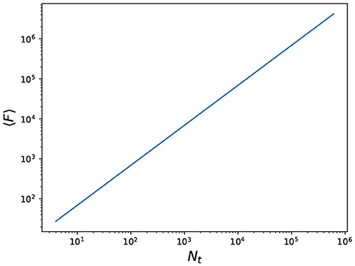
Figure 3. Mean first-passage time for scale-free network vs. the number of vertices N_t.

In [44], the author consider the mean community time.

4. Conclusion and Discussion

In summary, we have proposed our scale-free networks by introducing a graphic operation, i.e., rectangle operation. And then, we have presented a comprehensive and systematical analysis of mean first-passage time on random walks of our scale-free networks. We have provided an explicit expression of mean first-passage time on random walks, which is associated with effective resistances for the network. Our networks demonstrate the importance and influence of heterogeneous network topology in random walk behavior, there by providing insights for designing real networks with small mean first-passage time. We believe that our methods will not only allow for the extension of random walks analysis to some of the very large networks, but also provide another perspective for understanding the property of networks.

Data Availability Statement

The original contributions presented in the study are included in the article/supplementary material, further inquiries can be directed to the corresponding author/s.

Author Contributions

XW provided this topic and wrote the paper. JS modified and discussed and drew all figures. FM discussed and BY guided the manuscript. All authors contributed to manuscript and approved the submitted version.

Funding

This research was supported by the National Key Research and Development Plan under Grant No. 2019YFA0706401, the National Natural Science Foundation of China under Grant Nos. 61632002, 61872399, 61872166, 61672264, and 61662066, and the National Natural Science Foundation of China Youth Project under Grant Nos. 61802009, 61902005, and 62002002.

Conflict of Interest

The authors declare that the research was conducted in the absence of any commercial or financial relationships that could be construed as a potential conflict of interest.

References

1. Watts DJ, Strogatz SH. Collective dynamics of small-world networks. Nature. (1998) 393:440–2. doi: 10.1038/30918

PubMed Abstract | CrossRef Full Text | Google Scholar

2. Barabási AL, Albert R. Emergence of scaling in random networks. Science. (1999) 5439:509–12. doi: 10.1126/science.286.5439.509

CrossRef Full Text | Google Scholar

3. Albert R, Barabási AL. Statistical mechanics of complex networks. Rev Mod Phys. (2002) 74:47–97. doi: 10.1103/RevModPhys.74.47

CrossRef Full Text | Google Scholar

4. Noh JD, Rieger H. Random walks on complex networks. Phys Rev Lett. (2004) 92:118701. doi: 10.1103/PhysRevLett.92.118701

PubMed Abstract | CrossRef Full Text | Google Scholar

5. Weng TF, Zhang J, Khajehnejad M, Small M, Zheng R, Hui P. Navigation by anomalous random walks on complex networks. Sci Rep. (2016) 6:1. doi: 10.1038/srep37547

PubMed Abstract | CrossRef Full Text | Google Scholar

6. Skardal PS, Adhikari S. Dynamics of nonlinear random walks on complex networks. J Nonlinear Sci. (2019) 29:1419–44. doi: 10.1007/s00332-018-9521-7

PubMed Abstract | CrossRef Full Text | Google Scholar

7. Pons P, Latapy M. Computing communities in large networks using random walks. Comput Inform Sci. (2005) 3733:284–93. doi: 10.1007/11569596_31

CrossRef Full Text | Google Scholar

8. Millán VML, Cholvi V, López L, Anta AF. A model of self-avoiding random walks for searching complex networks. Networks. (2012) 60:2. doi: 10.1002/net.20461

CrossRef Full Text | Google Scholar

9. Xie YY, Chang SH, Zhang ZP, Zhang M, Yang L. Efficient sampling of complex network with modified random walk strategies. Phys A Stat Mech Appl. (2018) 492:57–64. doi: 10.1016/j.physa.2017.09.032

CrossRef Full Text | Google Scholar

10. Arruda HF, Silva FN, Comin CH, Amancio DR, Costa LF. Connecting network science and information theory. Phys A Stat Mech Appl. (2019) 515:641–8. doi: 10.1016/j.physa.2018.10.005

CrossRef Full Text | Google Scholar

11. Pham TV. Orbits of rotor-router operation and stationary distribution of random walks on directed graphs. Adv Appl Math. (2015) 70:45–53. doi: 10.1016/j.aam.2015.06.006

CrossRef Full Text | Google Scholar

12. Sarma AD, Molla AR, Panduranganb G. Efficient random walk sampling in distributed networks. J Parallel Distrib Comput. (2015) 77:84–94. doi: 10.1016/j.jpdc.2015.01.002

CrossRef Full Text | Google Scholar

13. Cooper C, Radzik T, Siantos Y. Estimating network parameters using random walks. Soc Netw Anal Min. (2014) 4:168. doi: 10.1007/s13278-014-0168-6

CrossRef Full Text | Google Scholar

14. Liu YS, Zeng XX, He ZY, Zou Q. Inferring microRNA-Disease associations by random walk on a heterogeneous network with multiple data sources. IEEE ACM Trans Comput Biol Bioinform. (2017) 14:905–15. doi: 10.1109/TCBB.2016.2550432

PubMed Abstract | CrossRef Full Text | Google Scholar

15. Li Y, Zhang ZL. Random walks and Green's function on digraphs: a framework for estimating wireless transmission costs. IEEE ACM Trans Netw. (2013) 21:135–48. doi: 10.1109/TNET.2012.2191158

CrossRef Full Text | Google Scholar

16. Beraldi R. Biased random walks in uniform wireless networks. IEEE Trans Mobile Comput. (2009) 8:500–13. doi: 10.1109/TMC.2008.151

CrossRef Full Text | Google Scholar

17. Ribeiro B, Wang P, Murai F, Towsley D. Sampling directed graphs with random walks. Proc IEEE INFOCOM. (2012) 1692–700. doi: 10.1109/INFCOM.2012.6195540

CrossRef Full Text | Google Scholar

18. Zheng H, Yang F, Tian X, Gan X, Wang X, Xiao S. Data gathering with compressive sensing in wireless sensor networks: a random walk based approach. IEEE Trans Parallel Distrib Syst. (2015) 26:35–44. doi: 10.1109/TPDS.2014.2308212

CrossRef Full Text | Google Scholar

19. Casa Grande HL, Cotacallapa M, Hase MO. Random walk in degree space and the time-dependent Watts-Strogatz model. Phys Rev E. (2017) 95:012321. doi: 10.1103/PhysRevE.95.012321

PubMed Abstract | CrossRef Full Text | Google Scholar

20. Lambiotte R, Delvenne JC, Barahona M. Random walks, Markov processes and the multiscale modular organization of complex networks. IEEE Trans Netw Sci Eng. (2014) 1:76–90. doi: 10.1109/TNSE.2015.2391998

CrossRef Full Text | Google Scholar

21. Qu Y, Guan XH, Zheng QH, Liu T, Wang LD, Hou YQ, et al. Exploring community structure of software Call Graph and its applications in class cohesion measurement. J Syst Softw. (2015) 108:193–210. doi: 10.1016/j.jss.2015.06.015

CrossRef Full Text | Google Scholar

22. Shang Y. Consensus in averager-copier-voter networks of moving dynamical agents. Chaos. (2017) 27:023116. doi: 10.1063/1.4976959

PubMed Abstract | CrossRef Full Text | Google Scholar

23. Gamarnik D. On deciding stability of constrained homogeneous random walks and queueing systems. Math Oper Res. (2002) 27:272–93. doi: 10.1287/moor.27.2.272.321

CrossRef Full Text | Google Scholar

24. Sarwate AD, Dimakis AG. The impact of mobility on gossip algorithms. IEEE Trans Inform Theor. (2012) 58:1731–42. doi: 10.1109/TIT.2011.2177753

CrossRef Full Text | Google Scholar

25. Maier BF, Brockmann D. Cover time for random walks on arbitrary complex networks. Phys Rev E. (2017) 96:042307. doi: 10.1103/PhysRevE.96.042307

PubMed Abstract | CrossRef Full Text | Google Scholar

26. Jing XL, Zhao CH, Ling X. Mean first passage time and average trapping time for random walks on weighted networks. Complex Syst. (2018) 15:4. doi: 10.13306/j.1672-3813.2018.04.004

CrossRef Full Text

27. Newman MEJ. Spectra of networks containing short loops. Phys Rev E. (2019) 100:012314. doi: 10.1103/PhysRevE.100.012314

PubMed Abstract | CrossRef Full Text | Google Scholar

28. Newman MEJ, Zhang X, Nadakuditi RR. Spectra of random networks with arbitrary degrees. Phys Rev E. (2019) 99:042309. doi: 10.1103/PhysRevE.99.042309

PubMed Abstract | CrossRef Full Text | Google Scholar

29. Cvetkovic DM, Doob M, Sachs H. Spectra of Graphs, Theory and Application. Heidelberg: Johann Ambrosius Barth (1995).

Google Scholar

30. Bondy JA, Murty USR. Graph Theory With Applications. New York, NY: American Elsevier (1976).

Google Scholar

31. Foster RM. The average impedance of an electrical network. In: Edwards JW, ediotr. Reissner Anniversary Volume, Contributions to Applied Mechanics. Ann Arbor, MI (1948). p. 333–40.

32. Chen H. Random walks and the effective resistance sum rules. Discrete Appl Math. (2010) 158:1691–700. doi: 10.1016/j.dam.2010.05.020

CrossRef Full Text | Google Scholar

33. Chen H, Zhang F. Resistance distance and the normalized Laplacian spectrum. Discrete Appl Math.(2007) 155:654–61. doi: 10.1016/j.dam.2006.09.008

CrossRef Full Text | Google Scholar

34. Gutman I, Feng L, Yu G. Degree resistance distance of unicyclic graphs. Trans Combinator.(2012) 1:27–40.

Google Scholar

35. Gutman I, Mohar B. The quasi-Wiener and the Kirchhoff indices coincide. J Chem Inform Comput Sci. (1996) 36:982–5. doi: 10.1021/ci960007t

CrossRef Full Text | Google Scholar

36. Liu Q. Some results of resistance distance and Kirchhoff index of subdivision vertex-edge corona for graphs. Adv Math. (2016) 45:176–84. doi: 10.11845/sxjz.2015128b

CrossRef Full Text

37. Liu Q. Some results of resistance distance and Kirchhoff index based on R-graph. IAENG Int J Appl Math. (2016) 46:346–52.

Google Scholar

38. Liu Q, Liu JB, Cao JD. The Laplacian polynomial and Kirchhoff index of graphs based on R-graphs. Neurocomputing. (2016) 177:441–6. doi: 10.1016/j.neucom.2015.11.060

CrossRef Full Text | Google Scholar

39. Kemeny JG, Snell JL. Finite Markov Chains. New York, NY: Springer (1976).

Google Scholar

40. Wang XM, Ma F. Constructions and properties of a class of random scale-free networks. Chaos. (2020) 30:043120. doi: 10.1063/1.5123594

PubMed Abstract | CrossRef Full Text | Google Scholar

41. Zhang ZZ, Zhou SG, Zou T, Chen LC, Guan JH. Different thresholds of bond percolation in scale-free networks with identical degree sequence. Phys Rev E. (2009) 79:031110. doi: 10.1103/PhysRevE.79.031110

PubMed Abstract | CrossRef Full Text | Google Scholar

42. Ma F, Wang XM, Wang P. An ensemble of random graphs with identical degree distribution. Chaos. (2020) 30:013136. doi: 10.1063/1.5105354

PubMed Abstract | CrossRef Full Text | Google Scholar

43. Sheng YB, Zhang ZZ. Low-mean hitting time for random walks on heterogeneous networks. IEEE Trans Inform Theor. (2019) 65:11. doi: 10.1109/TIT.2019.2925610

CrossRef Full Text | Google Scholar

44. Shang Y. Mean commute time for random walks on hierarchical scale-free networks. Intern Math. (2012) 8:321–37. doi: 10.1080/15427951.2012.685685

CrossRef Full Text | Google Scholar