Error Propagation of Capon’s Minimum Variance Estimator

1 Introduction

The reconstruction of model parameters from a given set of measurements is one of the most important tasks in geophysical and space science studies. The measurements are always affected by measurement errors which result in estimation errors for the wanted model parameters. The Capon method [1–3], also known as minimum variance distortionless response estimator (MVDR), is currently being considered as a robust inversion method for the analysis of planetary magnetic fields. In the past, the method has successfully been applied to the analysis of waves [1, 4] and therefore, specific attention has been paid to errors of the spectrum resulting from random perturbations in the amplitude and phase of sensor arrays [5]. Since Capon’s method is based on the evaluation of statistically averaged data, the spectrum is also affected by errors resulting from a finite number of samples [6]. Within the estimation of the frequency-wavenumber spectrum, the difference between static structures and waves or their combination can be discerned through dispersion relation analysis [7–12]. Concerning the application of the Capon method for the analysis of planetary magnetic fields, the error propagation of Capon’s estimator itself is of major importance for assessing the quality of the reconstructed model parameters. In general, two essential types of errors are expectable. On the one hand, the measured magnetic field data are affected by e.g., offsets, gains resulting from thermal variations and spacecraft magnetic disturbances [13]. On the other hand, the determination of the spacecraft’s positions can be defective (measurement position errors), which results in a defective shape matrix. As a follow-up of the generalized derivation of Capon’s method [3] and the error estimation of the power spectrum [6], in this work the effects of measurement errors, measurement position errors as well as finite sample sizes on Capon’s estimator are considered.

2 Capon’s Method

Before deducing the error propagation of Capon’s method, the main ideas of the method are shortly revisited [2, 3]. Due to the complexity of several physical problems, the entire parametrization of experimental data is unrealizable. Thus, it is useful to decompose the measurements $\underset{¯}{B}$ into parametrized parts $\underset{¯}{\underset{¯}{H}}\underset{¯}{g}$, where $\underset{¯}{g}$ contains the corresponding wanted model coefficients and the shape matrix $\underset{¯}{\underset{¯}{H}}$ describes the distribution of the measurement positions with respect to the underlying model, non-parametrized parts $\underset{¯}{v}$ as well as measurement noise $\underset{¯}{n}$, so that

$\underset{¯}{B}=\underset{¯}{\underset{¯}{H}}\underset{¯}{g}+\underset{¯}{v}+\underset{¯}{n}(1)$

is valid. The measurement noise is assumed to be Gaussian with variance ${\sigma }_n$ and zero mean $\left(\langle \underset{¯}{n}\rangle =0\right)$. Since the shape matrix $\underset{¯}{\underset{¯}{H}}$ is not invertible and the non-parametrized parts are unknown, the exact solution for the wanted model coefficients $\underset{¯}{g}$ is not available in general. Capon’s method delivers an estimator ${\underset{¯}{g}}_C$ for the ideal solution $\underset{¯}{g}$. The method is based on the construction of a filter matrix $\underset{¯}{\underset{¯}{w}}$, that minimizes the output power

$\text{tr}\left[{\underset{¯}{\underset{¯}{w}}}^{†}\underset{¯}{\underset{¯}{M}}\underset{¯}{\underset{¯}{w}}\right](2)$

with respect to the distortionless constraint

${\underset{¯}{\underset{¯}{w}}}^{†}\underset{¯}{\underset{¯}{H}}=\underset{¯}{\underset{¯}{I}}(3)$

where $\text{tr}\left[{\underset{¯}{\underset{¯}{w}}}^{†}\underset{¯}{\underset{¯}{M}}\underset{¯}{\underset{¯}{w}}\right]$ is the trace of the matrix ${\underset{¯}{\underset{¯}{w}}}^{†}\underset{¯}{\underset{¯}{M}}\underset{¯}{\underset{¯}{w}}$ and $\underset{¯}{\underset{¯}{I}}$ is the identity matrix. The matrix $\underset{¯}{\underset{¯}{M}}=\langle \underset{¯}{B}\circ \underset{¯}{B}\rangle$ denotes the data covariance matrix. Capon’s estimator realizing the minimal output power results in

${\underset{¯}{g}}_C={\underset{¯}{\underset{¯}{w}}}^{†}\langle \underset{¯}{B}\rangle ={\left[{\underset{¯}{\underset{¯}{H}}}^{†}{\underset{¯}{\underset{¯}{M}}}^{-1}\underset{¯}{\underset{¯}{H}}\right]}^{-1}{\underset{¯}{\underset{¯}{H}}}^{†}{\underset{¯}{\underset{¯}{M}}}^{-1}\langle \underset{¯}{B}\rangle .(4)$

The robustness of the method can be improved by the diagonal loading technique $\underset{¯}{\underset{¯}{M}}\to \underset{¯}{\underset{¯}{M}}+{\sigma }_d^2\underset{¯}{\underset{¯}{I}}$, where ${\sigma }_d$ is the so called diagonal loading parameter [3]. Thus, the estimator depends on the measurements and on the measurement positions so that measurement errors as well as measurement position errors transfer onto the estimator.

3 Error Propagation

In the following, the error propagation of Capon’s estimator is deduced. Since it is expectable that the errors are much smaller than the measurements themselves, the error propagation is derived by making use of a linearization. For the approximation of the matrix inversions that are necessary for calculating Capon’s estimator, the Neumann series bears of essential meaning for which reason we discuss it in a seperate section.

3.1 Neumann Series

The Neumann series is a special case of the functional calculus for linear operators or matrices, respectively, [14] and enables the approximation of matrix inversions.

Let $\underset{¯}{\underset{¯}{T}}$ denote a bounded matrix with norm $\Vert \underset{¯}{\underset{¯}{T}}\Vert <1$. Then,

${\left[\underset{¯}{\underset{¯}{I}}-\underset{¯}{\underset{¯}{T}}\right]}^{-1}={\displaystyle \sum }_{k=0}^{\infty }{\underset{¯}{\underset{¯}{T}}}^k=\underset{¯}{\underset{¯}{I}}+\underset{¯}{\underset{¯}{T}}+\mathrm{}\left({\Vert \underset{¯}{T}\Vert }^2\right)(5)$

where $\underset{¯}{\underset{¯}{I}}$ is the identity matrix and ${\underset{¯}{\underset{¯}{T}}}^k$ denotes the k’th power of the matrix $\underset{¯}{\underset{¯}{T}}$. The demand $\Vert \underset{¯}{\underset{¯}{T}}\Vert <1$ guarantees the convergence of the series. Thus, the Neumann series can be understood as a generalization of the geometric series for linear operators.

As a direct consequence it follows that

${\left[\underset{¯}{\underset{¯}{I}}+\underset{¯}{\underset{¯}{T}}\right]}^{-1}={\left[\underset{¯}{\underset{¯}{I}}-\left(-\underset{¯}{\underset{¯}{T}}\right)\right]}^{-1}={\displaystyle \sum }_{k=0}^{\infty }{\left(-1\right)}^k{\underset{¯}{\underset{¯}{T}}}^k=\underset{¯}{\underset{¯}{I}}-\underset{¯}{\underset{¯}{T}}+\mathrm{}\left({\Vert \underset{¯}{\underset{¯}{T}}\Vert }^2\right).(6)$

For the estimation of Capon’s error propagation a generalized formulation of the Neumann series is required. To expand the inverse of the sum of a matrix $\underset{¯}{\underset{¯}{S}}$ and a matrix $\underset{¯}{\underset{¯}{T}}$, where it is assumed that $\underset{¯}{\underset{¯}{S}}$ is invertible, the sum can be rewritten as

$\underset{¯}{\underset{¯}{S}}+\underset{¯}{\underset{¯}{T}}=\underset{¯}{\underset{¯}{S}}\left(\underset{¯}{\underset{¯}{I}}+{\underset{¯}{\underset{¯}{S}}}^{-1}\underset{¯}{\underset{¯}{T}}\right).(7)$

If $\Vert {\underset{¯}{\underset{¯}{S}}}^{-1}\underset{¯}{\underset{¯}{T}}\Vert <1$, the Neumann series can be applied to the sum $\underset{¯}{\underset{¯}{I}}+{\underset{¯}{\underset{¯}{S}}}^{-1}\underset{¯}{\underset{¯}{T}}$ resulting in

$\begin{array}{c}{\left[\underset{¯}{\underset{¯}{S}}+\underset{¯}{\underset{¯}{T}}\right]}^{-1}={\left[\underset{¯}{\underset{¯}{S}}\left(\underset{¯}{\underset{¯}{I}}+{\underset{¯}{\underset{¯}{S}}}^{-1}\underset{¯}{\underset{¯}{T}}\right)\right]}^{-1}={\left(\underset{¯}{\underset{¯}{I}}+{\underset{¯}{\underset{¯}{S}}}^{-1}\underset{¯}{\underset{¯}{T}}\right)}^{-1}{\underset{¯}{\underset{¯}{S}}}^{-1}\\ =\left[\stackrel{\infty }{{\displaystyle \sum }_{k=0}}{\left(-1\right)}^k{\left({\underset{¯}{\underset{¯}{S}}}^{-1}\underset{¯}{\underset{¯}{T}}\right)}^k\right]{\underset{¯}{\underset{¯}{S}}}^{-1}\\ ={\underset{¯}{\underset{¯}{S}}}^{-1}-{\underset{¯}{\underset{¯}{S}}}^{-1}\underset{¯}{\underset{¯}{T}}{\underset{¯}{\underset{¯}{S}}}^{-1}+\mathrm{}\left({\Vert {\underset{¯}{\underset{¯}{S}}}^{-1}\underset{¯}{\underset{¯}{T}}\Vert }^2\right).\end{array}(8)$

3.2 Measurement Errors

In the following, the error of Capon’s estimator resulting from measurement errors is derived. The model for the (temporal) statistically averaged accurate data $\langle \underset{¯}{B}\rangle$ without measurement errors is given by

$\langle \underset{¯}{B}\rangle =\underset{¯}{\underset{¯}{H}}\underset{¯}{g}+\langle \underset{¯}{v}\rangle ,(9)$

where $\underset{¯}{g}$ is the wanted coefficient vector, $\underset{¯}{\underset{¯}{H}}$ denotes the shape matrix which describes the spatial dependence of the measurement positions with respect to the underlying model and $\langle \underset{¯}{v}\rangle$ denotes the (temporal) statistically averaged parts of the measurements that are not parametrized by the model $\underset{¯}{\underset{¯}{H}}\underset{¯}{g}$ [3]. The corresponding accurate estimator resulting from Capon’s method is given by

${\underset{¯}{g}}_C={\underset{¯}{\underset{¯}{w}}}^{†}\langle \underset{¯}{B}\rangle (10)$

where

${\underset{¯}{\underset{¯}{w}}}^{†}={\left[{\underset{¯}{\underset{¯}{H}}}^{†}{\underset{¯}{\underset{¯}{M}}}^{-1}\underset{¯}{\underset{¯}{H}}\right]}^{-1}{\underset{¯}{\underset{¯}{H}}}^{†}{\underset{¯}{\underset{¯}{M}}}^{-1}(11)$

denotes the accurate filter matrix composed of the shape matrix $\underset{¯}{\underset{¯}{H}}$ and the data covariance matrix $\underset{¯}{\underset{¯}{M}}=\langle \underset{¯}{B}\circ \underset{¯}{B}\rangle$ [3].

The perturbed measurements $\widetilde{\underset{¯}{B}}$ can be rewritten as

$\widetilde{\underset{¯}{B}}=\underset{¯}{B}+\delta \underset{¯}{B},(12)$

where $\delta \underset{¯}{B}$ denotes the measurement error. Because of the linearity of the averaging process, the perturbed averaged measurements $\langle \widetilde{\underset{¯}{B}}\rangle$ are given by

$\langle \widetilde{\underset{¯}{B}}\rangle =\langle \underset{¯}{B}\rangle +\langle \delta \underset{¯}{B}\rangle (13)$

where $\langle \delta \underset{¯}{B}\rangle$ denotes the statistically averaged measurement error. The corresponding perturbed estimator results in

${\underset{¯}{\tilde{g}}}_C={\underset{¯}{\underset{¯}{\tilde{w}}}}^{†}\langle \widetilde{\underset{¯}{B}}\rangle (14)$

where

${\underset{¯}{\underset{¯}{\tilde{w}}}}^{†}={\left[{\underset{¯}{\underset{¯}{H}}}^{†}{\underset{¯}{\underset{¯}{\tilde{M}}}}^{-1}\underset{¯}{\underset{¯}{H}}\right]}^{-1}{\underset{¯}{\underset{¯}{H}}}^{†}{\underset{¯}{\underset{¯}{\tilde{M}}}}^{-1}(15)$

denotes the perturbed filter matrix. Thus, the difference between the accurate and the perturbed estimator results in

$\begin{array}{c}{\underset{¯}{g}}_C-{\underset{¯}{\tilde{g}}}_C={\underset{¯}{\underset{¯}{w}}}^{†}\langle \underset{¯}{B}\rangle -{\underset{¯}{\underset{¯}{\tilde{w}}}}^{†}\langle \widetilde{\underset{¯}{B}}\rangle ={\underset{¯}{\underset{¯}{w}}}^{†}\langle \widetilde{\underset{¯}{B}}\rangle -{\underset{¯}{\underset{¯}{w}}}^{†}\langle \delta \underset{¯}{B}\rangle -{\underset{¯}{\underset{¯}{\tilde{w}}}}^{†}\langle \widetilde{\underset{¯}{B}}\rangle \\ =\left({\underset{¯}{\underset{¯}{w}}}^{†}-{\underset{¯}{\underset{¯}{\tilde{w}}}}^{†}\right)\langle \widetilde{\underset{¯}{B}}\rangle -{\underset{¯}{\underset{¯}{w}}}^{†}\langle \delta \underset{¯}{B}\rangle \end{array}(16)$

Within the practical application only the perturbed measurements $\langle \widetilde{\underset{¯}{B}}\rangle$ are known and thus, only the filter matrix ${\underset{¯}{\underset{¯}{\tilde{w}}}}^{†}$ is known. For the calculation of the difference between the two filter matrices, in the following a linearized approximation is applied. By means of Eq. 12, the unknown accurate data covariance matrix can be rewritten as

$\begin{array}{c}\underset{¯}{\underset{¯}{M}}=\langle \underset{¯}{B}\circ \underset{¯}{B}\rangle =\langle \left(\underset{¯}{\tilde{B}}-\delta \underset{¯}{B}\right)\circ \left(\underset{¯}{\tilde{B}}-\delta \underset{¯}{B}\right)\rangle \\ =\underset{¯}{\underset{¯}{\tilde{M}}}-2\langle \underset{¯}{\tilde{B}}\rangle \circ \langle \delta \underset{¯}{B}\rangle +\langle \delta \underset{¯}{B}\circ \delta \underset{¯}{B}\rangle \end{array}(17)$

where $\underset{¯}{\underset{¯}{\tilde{M}}}=\langle \underset{¯}{\tilde{B}}\circ \underset{¯}{\tilde{B}}\rangle$. We assume, that the measurement errors are much smaller than the measurements themselves, i.e., $\left|\delta \underset{¯}{B}\right|\ll \left|\underset{¯}{\tilde{B}}\right|$. This assumption is surely justified in the majority of applications. Considering for example the analysis of planetary magnetic fields, the measurement errors are smaller than $1\text{nT}$, so that $\left|\delta \underset{¯}{B}\right|/\left|\underset{¯}{\tilde{B}}\right|<1\text{\%}$. Thus, in the following all terms being quadratic within the errors (e.g., $\langle \delta \underset{¯}{B}\circ \delta \underset{¯}{B}\rangle$) will be neglected, so that the data covariance matrix results in

$\underset{¯}{\underset{¯}{M}}=\underset{¯}{\underset{¯}{\tilde{M}}}-2\langle \underset{¯}{\tilde{B}}\rangle \circ \langle \delta \underset{¯}{B}\rangle =:\underset{¯}{\underset{¯}{\tilde{M}}}+\text{Δ}\underset{¯}{\underset{¯}{M}}.(18)$

In the case of ${\Vert {\underset{¯}{\underset{¯}{\tilde{M}}}}^{-1}\text{Δ}\underset{¯}{\underset{¯}{M}}\Vert }_2<1$, where ${\Vert .\Vert }_2$ denotes the spectral norm, the application of the Neumann series (Section 3.1) delivers

${\underset{¯}{\underset{¯}{M}}}^{-1}={(\underset{¯}{\underset{¯}{\tilde{M}}}+\text{Δ}\underset{¯}{\underset{¯}{M}})}^{-1}\approx {\underset{¯}{\underset{¯}{\tilde{M}}}}^{-1}-{\underset{¯}{\underset{¯}{\tilde{M}}}}^{-1}\text{Δ}\underset{¯}{\underset{¯}{M}}{\underset{¯}{\underset{¯}{\tilde{M}}}}^{-1}(19)$

as well as

$\begin{array}{c}\underset{¯}{\underset{¯}{P}}={\left[{\underset{¯}{\underset{¯}{H}}}^{†}{\underset{¯}{\underset{¯}{M}}}^{-1}\underset{¯}{\underset{¯}{H}}\right]}^{-1}\stackrel{\left(19\right)}{=}{\left[{\underset{¯}{\underset{¯}{H}}}^{†}{\underset{¯}{\underset{¯}{\tilde{M}}}}^{-1}\underset{¯}{\underset{¯}{H}}-{\underset{¯}{\underset{¯}{H}}}^{†}{\underset{¯}{\underset{¯}{\tilde{M}}}}^{-1}\text{Δ}\underset{¯}{\underset{¯}{M}}{\underset{¯}{\underset{¯}{\tilde{M}}}}^{-1}\underset{¯}{\underset{¯}{H}}\right]}^{-1}\\ ={\left[{\underset{¯}{\underset{¯}{H}}}^{†}{\underset{¯}{\underset{¯}{\tilde{M}}}}^{-1}\underset{¯}{\underset{¯}{H}}\right]}^{-1}+{\left[{\underset{¯}{\underset{¯}{H}}}^{†}{\underset{¯}{\underset{¯}{\tilde{M}}}}^{-1}\underset{¯}{\underset{¯}{H}}\right]}^{-1}{\underset{¯}{\underset{¯}{H}}}^{†}{\underset{¯}{\underset{¯}{\tilde{M}}}}^{-1}\text{Δ}\underset{¯}{\underset{¯}{M}}{\underset{¯}{\underset{¯}{\tilde{M}}}}^{-1}\underset{¯}{\underset{¯}{H}}{\left[{\underset{¯}{\underset{¯}{H}}}^{†}{\underset{¯}{\underset{¯}{\tilde{M}}}}^{-1}\underset{¯}{\underset{¯}{H}}\right]}^{-1}\\ =\underset{¯}{\underset{¯}{\tilde{P}}}+\underset{¯}{\underset{¯}{\tilde{P}}}{\underset{¯}{\underset{¯}{H}}}^{†}{\underset{¯}{\underset{¯}{\tilde{M}}}}^{-1}\text{Δ}\underset{¯}{\underset{¯}{M}}{\underset{¯}{\underset{¯}{\tilde{M}}}}^{-1}\underset{¯}{\underset{¯}{H}}\underset{¯}{\underset{¯}{\tilde{P}}}\end{array}(20)$

for the unknown coefficient matrix $\underset{¯}{\underset{¯}{P}}$ [3]. Using

${\underset{¯}{\underset{¯}{H}}}^{†}{\underset{¯}{\underset{¯}{M}}}^{-1}={\underset{¯}{\underset{¯}{H}}}^{†}{\underset{¯}{\underset{¯}{\tilde{M}}}}^{-1}-{\underset{¯}{\underset{¯}{H}}}^{†}{\underset{¯}{\underset{¯}{\tilde{M}}}}^{-1}\text{Δ}\underset{¯}{\underset{¯}{M}}{\underset{¯}{\underset{¯}{\tilde{M}}}}^{-1}(21)$

it follows that

$\begin{array}{c}{\underset{¯}{\underset{¯}{w}}}^{†}=\underset{¯}{\underset{¯}{P}}{\underset{¯}{\underset{¯}{H}}}^{†}{\underset{¯}{\underset{¯}{M}}}^{-1}\\ =\left[\underset{¯}{\underset{¯}{\tilde{P}}}+\underset{¯}{\underset{¯}{\tilde{P}}}{\underset{¯}{\underset{¯}{H}}}^{†}{\underset{¯}{\underset{¯}{\tilde{M}}}}^{-1}\text{Δ}\underset{¯}{\underset{¯}{M}}{\underset{¯}{\underset{¯}{\tilde{M}}}}^{-1}\underset{¯}{\underset{¯}{H}}\underset{¯}{\underset{¯}{\tilde{P}}}\right]\cdot \left[{\underset{¯}{\underset{¯}{H}}}^{†}{\underset{¯}{\underset{¯}{\tilde{M}}}}^{-1}-{\underset{¯}{\underset{¯}{H}}}^{†}{\underset{¯}{\underset{¯}{\tilde{M}}}}^{-1}\text{Δ}\underset{¯}{\underset{¯}{M}}{\underset{¯}{\underset{¯}{\tilde{M}}}}^{-1}\right]\\ =\underset{¯}{\underset{¯}{\tilde{P}}}{\underset{¯}{\underset{¯}{H}}}^{†}{\underset{¯}{\underset{¯}{\tilde{M}}}}^{-1}-\underset{¯}{\underset{¯}{\tilde{P}}}{\underset{¯}{\underset{¯}{H}}}^{†}{\underset{¯}{\underset{¯}{\tilde{M}}}}^{-1}\text{Δ}\underset{¯}{\underset{¯}{M}}{\underset{¯}{\underset{¯}{\tilde{M}}}}^{-1}+\\ \underset{¯}{\underset{¯}{\tilde{P}}}{\underset{¯}{\underset{¯}{H}}}^{†}{\underset{¯}{\underset{¯}{\tilde{M}}}}^{-1}\text{Δ}\underset{¯}{\underset{¯}{M}}{\underset{¯}{\underset{¯}{\tilde{M}}}}^{-1}\underset{¯}{\underset{¯}{H}}\underset{¯}{\underset{¯}{\tilde{P}}}{\underset{¯}{\underset{¯}{H}}}^{†}{\underset{¯}{\underset{¯}{\tilde{M}}}}^{-1}+\mathrm{}\left({\Vert \text{Δ}\underset{¯}{\underset{¯}{\tilde{M}}}\Vert }^2\right)\\ ={\underset{¯}{\underset{¯}{\tilde{w}}}}^{†}-{\underset{¯}{\underset{¯}{\tilde{w}}}}^{†}\text{Δ}\underset{¯}{\underset{¯}{M}}{\underset{¯}{\underset{¯}{\tilde{M}}}}^{-1}+{\underset{¯}{\underset{¯}{\tilde{w}}}}^{†}\text{Δ}\underset{¯}{\underset{¯}{M}}{\underset{¯}{\underset{¯}{\tilde{M}}}}^{-1}\underset{¯}{\underset{¯}{H}}{\underset{¯}{\underset{¯}{\tilde{w}}}}^{†}\\ ={\underset{¯}{\underset{¯}{\tilde{w}}}}^{†}+{\underset{¯}{\underset{¯}{\tilde{w}}}}^{†}\text{Δ}\underset{¯}{\underset{¯}{M}}{\underset{¯}{\underset{¯}{\tilde{M}}}}^{-1}\left(\underset{¯}{\underset{¯}{H}}{\underset{¯}{\underset{¯}{\tilde{w}}}}^{†}-\underset{¯}{\underset{¯}{I}}\right),\end{array}(22)$

where $\underset{¯}{\underset{¯}{I}}$ again denotes the identity matrix. Thus, the difference between the filter matrices can be approximated by

${\underset{¯}{\underset{¯}{w}}}^{†}-{\underset{¯}{\underset{¯}{\tilde{w}}}}^{†}={\underset{¯}{\underset{¯}{\tilde{w}}}}^{†}\text{Δ}\underset{¯}{\underset{¯}{M}}{\underset{¯}{\underset{¯}{\tilde{M}}}}^{-1}\left(\underset{¯}{\underset{¯}{H}}{\underset{¯}{\underset{¯}{\tilde{w}}}}^{†}-\underset{¯}{\underset{¯}{I}}\right).(23)$

Inserting this approximation into Eq. 16 delivers

${\underset{¯}{g}}_C-{\underset{¯}{\tilde{g}}}_C={\underset{¯}{\underset{¯}{\tilde{w}}}}^{†}\text{Δ}\underset{¯}{\underset{¯}{M}}{\underset{¯}{\underset{¯}{\tilde{M}}}}^{-1}\left(\underset{¯}{\underset{¯}{H}}{\underset{¯}{\underset{¯}{\tilde{w}}}}^{†}-\underset{¯}{\underset{¯}{I}}\right)\langle \underset{¯}{\tilde{B}}\rangle -{\underset{¯}{\underset{¯}{w}}}^{†}\langle \delta \underset{¯}{B}\rangle (24)$

where

${\underset{¯}{\underset{¯}{w}}}^{†}\langle \delta \underset{¯}{B}\rangle =\left[{\underset{¯}{\underset{¯}{\tilde{w}}}}^{†}+{\underset{¯}{\underset{¯}{\tilde{w}}}}^{†}\text{Δ}\underset{¯}{\underset{¯}{M}}{\underset{¯}{\underset{¯}{\tilde{M}}}}^{-1}\left(\underset{¯}{\underset{¯}{H}}{\underset{¯}{\underset{¯}{\tilde{w}}}}^{†}-\underset{¯}{\underset{¯}{I}}\right)\right]\langle \delta \underset{¯}{B}\rangle ={\underset{¯}{\underset{¯}{\tilde{w}}}}^{†}\langle \delta \underset{¯}{B}\rangle (25)$

within the linear approximation. Further transformation for estimating the relative error of the estimator delivers

$\begin{array}{c}{\underset{¯}{g}}_C-{\underset{¯}{\tilde{g}}}_C={\underset{¯}{\underset{¯}{\tilde{w}}}}^{†}\text{Δ}\underset{¯}{\underset{¯}{M}}{\underset{¯}{\underset{¯}{\tilde{M}}}}^{-1}\left(\underset{¯}{\underset{¯}{H}}{\underset{¯}{\underset{¯}{\tilde{w}}}}^{†}-\underset{¯}{\underset{¯}{I}}\right)\langle \underset{¯}{\tilde{B}}\rangle -{\underset{¯}{\underset{¯}{\tilde{w}}}}^{†}\langle \delta \underset{¯}{B}\rangle \\ ={\underset{¯}{\underset{¯}{\tilde{w}}}}^{†}\text{Δ}\underset{¯}{\underset{¯}{M}}{\underset{¯}{\underset{¯}{\tilde{M}}}}^{-1}\left(\underset{¯}{\underset{¯}{H}}{\underset{¯}{\underset{¯}{\tilde{w}}}}^{†}\langle \underset{¯}{\tilde{B}}\rangle -\langle \underset{¯}{\tilde{B}}\rangle \right)-{\underset{¯}{\underset{¯}{\tilde{w}}}}^{†}\langle \delta \underset{¯}{B}\rangle \\ ={\underset{¯}{\underset{¯}{\tilde{w}}}}^{†}\text{Δ}\underset{¯}{\underset{¯}{M}}{\underset{¯}{\underset{¯}{\tilde{M}}}}^{-1}\left(\underset{¯}{\underset{¯}{H}}{\underset{¯}{\tilde{g}}}_C-\langle \underset{¯}{\tilde{B}}\rangle \right)-{\underset{¯}{\underset{¯}{\tilde{w}}}}^{†}\langle \delta \underset{¯}{B}\rangle \\ ={\underset{¯}{\underset{¯}{\tilde{w}}}}^{†}\text{Δ}\underset{¯}{\underset{¯}{M}}{\underset{¯}{\underset{¯}{\tilde{M}}}}^{-1/2}{\underset{¯}{\underset{¯}{\tilde{M}}}}^{-1/2}\left(\underset{¯}{\underset{¯}{H}}{\underset{¯}{\tilde{g}}}_C-\langle \underset{¯}{\tilde{B}}\rangle \right)-{\underset{¯}{\underset{¯}{\tilde{w}}}}^{†}\langle \delta \underset{¯}{B}\rangle .\end{array}(26)$

Making use of the Cauchy-Schwarz inequality yields

${\left|{\underset{¯}{g}}_C-{\underset{¯}{\tilde{g}}}_C\right|}^2\le {\Vert {\underset{¯}{\underset{¯}{\tilde{w}}}}^{†}\text{Δ}\underset{¯}{\underset{¯}{M}}{\underset{¯}{\underset{¯}{\tilde{M}}}}^{-1/2}\Vert }_2^2\cdot {\Vert \underset{¯}{\underset{¯}{H}}{\underset{¯}{\tilde{g}}}_C-\langle \underset{¯}{\tilde{B}}\rangle \Vert }_{{\underset{¯}{\underset{¯}{\tilde{M}}}}^{-1}}^2+{\left|{\underset{¯}{\underset{¯}{\tilde{w}}}}^{†}\langle \delta \underset{¯}{B}\rangle \right|}^2,(27)$

where ${\Vert \underset{¯}{\underset{¯}{H}}{\underset{¯}{\tilde{g}}}_C-\langle \underset{¯}{\tilde{B}}\rangle \Vert }_{{\underset{¯}{\underset{¯}{\tilde{M}}}}^{-1}}^2={\left|{\underset{¯}{\underset{¯}{\tilde{M}}}}^{-1/2}\left(\underset{¯}{\underset{¯}{\tilde{H}}}{\underset{¯}{\tilde{g}}}_C-\langle \underset{¯}{\tilde{B}}\rangle \right)\right|}^2$. For the calculation of Capon’s estimator, the weighted difference $|{\underset{¯}{\underset{¯}{\tilde{M}}}}^{-1/2}\left(\underset{¯}{\underset{¯}{\tilde{H}}}{\underset{¯}{\tilde{g}}}_C-\langle \underset{¯}{\tilde{B}}\rangle \right){|}^2$ is minimized with respect to the unknown set of model parameters $\underset{¯}{\tilde{g}}$, resulting in $|{\underset{¯}{\underset{¯}{\tilde{M}}}}^{-1/2}\left(\underset{¯}{\underset{¯}{\tilde{H}}}{\underset{¯}{\tilde{g}}}_C-\langle \underset{¯}{\tilde{B}}\rangle \right){|}^2\sim {10}^{-7}$ [3]. A discussion about the calculation of the matrix ${\underset{¯}{\underset{¯}{M}}}^{-1/2}$ is given within the Appendix. Assuming that the weighted model mismatches are neglibigly small compared to the measurement errors, the deviation can be estimated upwards via

${\left|{\underset{¯}{g}}_C-{\underset{¯}{\tilde{g}}}_C\right|}^2\le {\left|{\underset{¯}{\underset{¯}{\tilde{w}}}}^{†}\langle \delta \underset{¯}{B}\rangle \right|}^2\le {\Vert {\underset{¯}{\underset{¯}{\tilde{w}}}}^{†}\Vert }_2^2\cdot {\left|\langle \delta \underset{¯}{B}\rangle \right|}^2,(28)$

or equivalently

$\frac{\left|{\underset{¯}{g}}_C-{\underset{¯}{\tilde{g}}}_C\right|}{\left|{\underset{¯}{g}}_C\right|}\le \frac{{\Vert {\underset{¯}{\underset{¯}{\tilde{w}}}}^{†}\Vert }_2\cdot \left|\langle \delta \underset{¯}{B}\rangle \right|}{\left|{\underset{¯}{g}}_C\right|}=\frac{{\Vert {\underset{¯}{\underset{¯}{\tilde{w}}}}^{†}\Vert }_2\cdot \left|\langle \delta \underset{¯}{B}\rangle \right|}{\left|{\underset{¯}{g}}_C\right|}\frac{\left|\langle \underset{¯}{B}\rangle \right|}{\left|\langle \underset{¯}{B}\rangle \right|}(29)$

for the relative error. When the measurements are adequately described by the underlying model, i.e., $\langle \underset{¯}{B}\rangle \approx \underset{¯}{\underset{¯}{H}}{\underset{¯}{g}}_C$, it follows that

$\frac{\left|{\underset{¯}{g}}_C-{\underset{¯}{\tilde{g}}}_C\right|}{\left|{\underset{¯}{g}}_C\right|}\le {\Vert {\underset{¯}{\underset{¯}{\tilde{w}}}}^{†}\Vert }_2\cdot {\Vert \underset{¯}{\underset{¯}{H}}\Vert }_2\frac{\left|\langle \delta \underset{¯}{B}\rangle \right|}{\left|\langle \underset{¯}{B}\rangle \right|}.(30)$

Comparing this expression with the relative error of the least square fit estimator [15].

$\frac{\left|{\underset{¯}{g}}_L-{\underset{¯}{\tilde{g}}}_L\right|}{\left|{\underset{¯}{g}}_L\right|}\le {\Vert {\underset{¯}{\underset{¯}{H}}}^{+}\Vert }_2\cdot {\Vert \underset{¯}{\underset{¯}{H}}\Vert }_2\frac{\left|\langle \delta \underset{¯}{B}\rangle \right|}{\left|\langle \underset{¯}{B}\rangle \right|},(31)$

where ${\underset{¯}{\underset{¯}{H}}}^{+}$ denotes the pseudoinverse of the shape matrix $\underset{¯}{\underset{¯}{H}}$, shows that the error propagation of Capon’s estimator follows the structure of the error propagation of the least square fit estimator. Since Capon’s method is based on the evaluation of averaged data, it can be seen that Gaussian errors with a vanishing mean value (i.e., $\langle \delta \underset{¯}{B}\rangle =0$) do not influence the estimator. Making use of the distortionless constraint [3].

${\underset{¯}{\underset{¯}{\tilde{w}}}}^{†}\underset{¯}{\underset{¯}{H}}=\underset{¯}{\underset{¯}{I}}(32)$

delivers

$\begin{array}{c}{\Vert {\underset{¯}{\underset{¯}{\tilde{w}}}}^{†}\Vert }_2=\underset{\underset{¯}{B}}{\text{max}}\frac{\left|{\underset{¯}{\underset{¯}{\tilde{w}}}}^{†}\underset{¯}{B}\right|}{\left|\underset{¯}{B}\right|}=\underset{\underset{¯}{\underset{¯}{H}}\underset{¯}{\tilde{g}}}{\text{max}}\frac{\left|{\underset{¯}{\underset{¯}{\tilde{w}}}}^{†}\underset{¯}{\underset{¯}{H}}\underset{¯}{\tilde{g}}\right|}{\left|\underset{¯}{\underset{¯}{H}}\underset{¯}{\tilde{g}}\right|}\\ =\underset{\underset{¯}{\tilde{g}}}{\text{max}}\frac{\left|\underset{¯}{\tilde{g}}\right|}{\left|\underset{¯}{\underset{¯}{H}}\underset{¯}{\tilde{g}}\right|}={\left(\underset{\underset{¯}{\tilde{g}}}{\text{min}}\frac{\left|\underset{¯}{\underset{¯}{H}}\underset{¯}{\tilde{g}}\right|}{\left|\underset{¯}{\tilde{g}}\right|}\right)}^{-1}\\ =\frac{1}{{\text{Σ}}_{\text{min}}}={\Vert {\underset{¯}{\underset{¯}{H}}}^{+}\Vert }_2,\end{array}(33)$

where ${\text{Σ}}_{\text{min}}$ denotes the smallest singular value of the shape matrix $\underset{¯}{\underset{¯}{H}}$ [15], i.e. $1/{\text{Σ}}_{\text{min}}$ describes the largest singular value of ${\underset{¯}{\underset{¯}{H}}}^{+}$. Using the definition of the condition number

$\kappa \left(\underset{¯}{\underset{¯}{H}}\right)=\frac{{\text{Σ}}_{\text{max}}}{{\text{Σ}}_{\text{min}}}={\Vert {\underset{¯}{\underset{¯}{H}}}^{+}\Vert }_2\cdot {\Vert \underset{¯}{\underset{¯}{H}}\Vert }_2={\Vert {\underset{¯}{\underset{¯}{w}}}^{†}\Vert }_2\cdot {\Vert \underset{¯}{\underset{¯}{H}}\Vert }_2\ge 1,(34)$

where ${\text{Σ}}_{\text{max}}$ denotes the largest singular value of the shape matrix $\underset{¯}{\underset{¯}{H}}$, yields

$\frac{\left|{\underset{¯}{g}}_C-{\underset{¯}{\tilde{g}}}_C\right|}{\left|{\underset{¯}{g}}_C\right|}\le \kappa \left(\underset{¯}{\underset{¯}{H}}\right)\frac{\left|\langle \delta \underset{¯}{B}\rangle \right|}{\left|\langle \underset{¯}{B}\rangle \right|}.(35)$

Thus, Capon’s estimator propagates the measurement errors in the same way as the least square fit estimator. This mathematical property can be interpreted as follows: These two methods differ in the filter matrices ${\underset{¯}{\underset{¯}{H}}}^{+}$ and ${\underset{¯}{\underset{¯}{w}}}^{†}$ which weight or eliminate parts of the data in different ways. Since these matrices are applied to the same set of measurements, which is characterized by a given measurement error, the different weighting of the data or the elimination of subsets does not reduce the errors, since the weighted data originate from the same ensemble. The upper bound of the relative estimation error is qualitatively sketched in Figure 1.

FIGURE 1

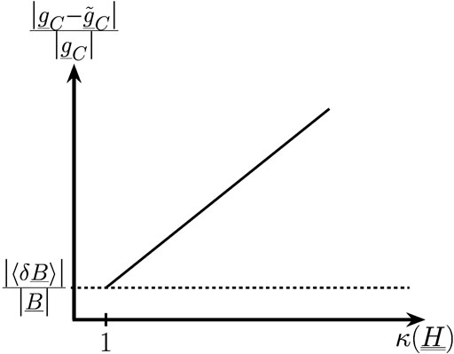
FIGURE 1. Sketch of the upper bound for the relative estimation error resulting from measurement errors with respect to the condition number $\kappa \left(\underset{¯}{\underset{¯}{H}}\right)$ of the shape matrix.

Furthermore, it should be noted that the condition number of the shape matrix determines how the measurement errors are amplified. Thereby, the condition number depends on the underlying model and the measurement positions, whereas the measurement error is produced by the sensor. For a given underlying model, the condition number solely depends on the measurement positions. Thus, the estimation errors can be reduced by analyzing measurements from suitable data points. Considering the analysis of Mercury’s magnetic field, the underlying model describes the geometry of the magnetic field, for example the internal dipole and quadrupole field [2, 3]. For the estimation of the corresponding Gauss coefficients [16, 17], the data points have to cover the geometry of the field properly. For example, the superposition of Mercury’s internal dipole field with the quadrupole field can equivalently be described as a northward shifted dipole field. When only measurement positions in the northern hemisphere are available, the condition number of the shape matrix increases, resulting in large estimation errors so that the internal field can be misinterpreted as a strong dipole field. The analysis of measurement points covering the southern and the northern hemisphere symmetrically, like that of the BepiColombo mission, decreases the condition number and enables a more detailed characterization of the geometry of Mercury’s internal magnetic field [18]. The smaller the condition number of the shape matrix becomes, the better the geometry of the field is covered by the data points [18].

Before discussing the errors resulting from the perturbed determination of the measurement positions, let us make a general comment about the error of Capon’s estimator resulting from measurement errors. The perturbed data can be rewritten in the form

$\langle \underset{¯}{\tilde{B}}\rangle =\langle \underset{¯}{B}\rangle +\langle \delta \underset{¯}{B}\rangle =\underset{¯}{\underset{¯}{H}}\underset{¯}{g}+\langle \underset{¯}{v}\rangle +\langle \delta \underset{¯}{B}\rangle =\underset{¯}{\underset{¯}{H}}\underset{¯}{g}+\langle \underset{¯}{\tilde{v}}\rangle ,(36)$

where $\langle \underset{¯}{\tilde{v}}\rangle =\langle \underset{¯}{v}\rangle +\langle \delta \underset{¯}{B}\rangle$. Since the filter matrix ${\underset{¯}{\underset{¯}{\tilde{w}}}}^{†}$ eliminates the non-parametrized parts from the total measured field [3], one might suppose that the measurement errors do not influence the estimation since these errors can as well be interpreted as non-parametrized parts. From the elimination of the non-parametrized parts

$0={\underset{¯}{\underset{¯}{\tilde{w}}}}^{†}\langle \underset{¯}{\tilde{v}}\rangle ={\underset{¯}{\underset{¯}{\tilde{w}}}}^{†}\langle \underset{¯}{v}\rangle +{\underset{¯}{\underset{¯}{\tilde{w}}}}^{†}\langle \delta \underset{¯}{B}\rangle (37)$

it does not follow that ${\underset{¯}{\underset{¯}{\tilde{w}}}}^{†}\langle \delta \underset{¯}{B}\rangle =0$. Since this term dominates the error of the estimator (cf. Eq. 28), the measurement errors are not eliminated by the filter matrix in general.

3.3 Measurement Position Errors

The model for the correctly determined measurement positions is given by

$\langle \underset{¯}{B}\rangle =\underset{¯}{\underset{¯}{H}}\underset{¯}{g}+\langle \underset{¯}{v}\rangle .(38)$

The corresponding accurate estimator results in

${\underset{¯}{g}}_C={\underset{¯}{\underset{¯}{w}}}^{†}\langle \underset{¯}{B}\rangle ,(39)$

where

${\underset{¯}{\underset{¯}{w}}}^{†}={\left[{\underset{¯}{\underset{¯}{H}}}^{†}{\underset{¯}{\underset{¯}{M}}}^{-1}\underset{¯}{\underset{¯}{H}}\right]}^{-1}{\underset{¯}{\underset{¯}{H}}}^{†}{\underset{¯}{\underset{¯}{M}}}^{-1}.(40)$

The perturbed determination of the sensor’s positions transfers onto a perturbed shape matrix $\underset{¯}{\underset{¯}{H}}$. Thus, the underlying model $\underset{¯}{\underset{¯}{H}}\underset{¯}{g}$ and the non-parametrized parts $\langle \underset{¯}{v}\rangle$ are perturbed so that the noisy model is given by

$\langle \underset{¯}{B}\rangle =\underset{¯}{\underset{¯}{\tilde{H}}}\underset{¯}{\tilde{g}}+\langle \underset{¯}{\tilde{v}}\rangle (41)$

and the corresponding perturbed estimator results in

${\underset{¯}{\tilde{g}}}_C={\underset{¯}{\underset{¯}{\tilde{w}}}}^{†}\langle \underset{¯}{B}\rangle ,(42)$

where

${\underset{¯}{\underset{¯}{\tilde{w}}}}^{†}={\left[{\underset{¯}{\underset{¯}{\tilde{H}}}}^{†}{\underset{¯}{\underset{¯}{M}}}^{-1}\underset{¯}{\underset{¯}{\tilde{H}}}\right]}^{-1}{\underset{¯}{\underset{¯}{\tilde{H}}}}^{†}{\underset{¯}{\underset{¯}{M}}}^{-1}.(43)$

The deviation between the accurate and the perturbed estimator results in

${\underset{¯}{g}}_C-{\underset{¯}{\tilde{g}}}_C=\left({\underset{¯}{\underset{¯}{w}}}^{†}-{\underset{¯}{\underset{¯}{\tilde{w}}}}^{†}\right)\langle \underset{¯}{B}\rangle .(44)$

As discussed above, only the perturbed filter matrix $\underset{¯}{\underset{¯}{\tilde{H}}}$ is known. Within a linear approximation, the unknown matrix $\underset{¯}{\underset{¯}{H}}$ can be rewritten as $\underset{¯}{\underset{¯}{H}}=\underset{¯}{\underset{¯}{\tilde{H}}}+\text{Δ}\underset{¯}{\underset{¯}{H}}$, where ${\Vert \text{Δ}\underset{¯}{\underset{¯}{H}}\Vert }_2\ll {\Vert \underset{¯}{\underset{¯}{\tilde{H}}}\Vert }_2$. For example, consider the shape matrix

$\underset{¯}{\underset{¯}{H}}=\left[\begin{array}{cc}1& {\left(\frac{R_{\text{M}}}{r_1}\right)}^3\\ 1& {\left(\frac{R_{\text{M}}}{r_2}\right)}^3\end{array}\right](45)$

which describes the magnetic field of a current sheet superposed with Mercury’s internal dipolar field [6], where $R_{\text{M}}$ indicates the planetary radius of Mercury and $r_1$ and $r_2$ are the measurement positions. The perturbed filter matrix is given by

$\underset{¯}{\underset{¯}{\tilde{H}}}=\left[\begin{array}{cc}1& {\left(\frac{R_{\text{M}}}{r_1+\text{Δ}{r}_1}\right)}^3\\ 1& {\left(\frac{R_{\text{M}}}{r_2+\text{Δ}{r}_2}\right)}^3\end{array}\right]=\left[\begin{array}{cc}1& \frac{R_{\text{M}}^3}{r_1^3{\left(1+\text{Δ}{r}_1/r_1\right)}^3}\\ 1& \frac{R_{\text{M}}^3}{r_2^3{\left(1+\text{Δ}{r}_2/r_2\right)}^3}\end{array}\right].(46)$

Assuming that $\text{Δ}{r}_i\ll r_i$, for $i=\mathrm{1,2}$, the perturbed matrix can be rewritten as

$\underset{¯}{\underset{¯}{\tilde{H}}}=\left[\begin{array}{cc}1& {\left(\frac{R_{\text{M}}}{r_1}\right)}^3\\ 1& {\left(\frac{R_{\text{M}}}{r_2}\right)}^3\end{array}\right]+\left[\begin{array}{cc}0& -3\frac{R_{\text{M}}^3}{r_1^3}\frac{\text{Δ}{r}_1}{r_1}\\ 0& -3\frac{R_{\text{M}}^3}{r_2^3}\frac{\text{Δ}{r}_2}{r_2}\end{array}\right]=\underset{¯}{\underset{¯}{H}}-\text{Δ}\underset{¯}{\underset{¯}{H}}(47)$

by making use of a Taylor series expansion. It should be noted that the shape matrix can be linearized for any underlying model by performing a Taylor series expansion for the functions within the model. Linearization of the error terms for the estimation of the unknown accurate filter matrix delivers

$\begin{array}{c}{\underset{¯}{\underset{¯}{w}}}^{†}\stackrel{\left(40\right)}{=}{\left[{\underset{¯}{\underset{¯}{H}}}^{†}{\underset{¯}{\underset{¯}{M}}}^{-1}\underset{¯}{\underset{¯}{H}}\right]}^{-1}{\underset{¯}{\underset{¯}{H}}}^{†}{\underset{¯}{\underset{¯}{M}}}^{-1}\\ ={\left[\left({\underset{¯}{\underset{¯}{\tilde{H}}}}^{†}+\text{Δ}{\underset{¯}{\underset{¯}{H}}}^{†}\right){\underset{¯}{\underset{¯}{M}}}^{-1}\left(\underset{¯}{\underset{¯}{\tilde{H}}}+\text{Δ}\underset{¯}{\underset{¯}{H}}\right)\right]}^{-1}\left({\underset{¯}{\underset{¯}{\tilde{H}}}}^{†}+\text{Δ}{\underset{¯}{\underset{¯}{H}}}^{†}\right){\underset{¯}{\underset{¯}{M}}}^{-1}\\ ={\left[{\underset{¯}{\underset{¯}{\tilde{H}}}}^{†}{\underset{¯}{\underset{¯}{M}}}^{-1}\left(\underset{¯}{\underset{¯}{\tilde{H}}}+\text{Δ}\underset{¯}{\underset{¯}{H}}\right)+\text{Δ}{\underset{¯}{\underset{¯}{H}}}^{†}{\underset{¯}{\underset{¯}{M}}}^{-1}\left(\underset{¯}{\underset{¯}{\tilde{H}}}+\text{Δ}\underset{¯}{\underset{¯}{H}}\right)\right]}^{-1}\left({\underset{¯}{\underset{¯}{\tilde{H}}}}^{†}+\text{Δ}{\underset{¯}{\underset{¯}{H}}}^{†}\right){\underset{¯}{\underset{¯}{M}}}^{-1}\\ ={\left[{\underset{¯}{\underset{¯}{\tilde{H}}}}^{†}{\underset{¯}{\underset{¯}{M}}}^{-1}\underset{¯}{\underset{¯}{\tilde{H}}}+{\underset{¯}{\underset{¯}{\tilde{H}}}}^{†}{\underset{¯}{\underset{¯}{M}}}^{-1}\text{Δ}\underset{¯}{\underset{¯}{H}}+\text{Δ}{\underset{¯}{\underset{¯}{H}}}^{†}{\underset{¯}{\underset{¯}{M}}}^{-1}\underset{¯}{\underset{¯}{\tilde{H}}}\right]}^{-1}\left({\underset{¯}{\underset{¯}{\tilde{H}}}}^{†}+\text{Δ}{\underset{¯}{\underset{¯}{H}}}^{†}\right){\underset{¯}{\underset{¯}{M}}}^{-1}.\end{array}(48)$

Making use of the Neumann series results in

$\begin{array}{l}{\left[{\underset{¯}{\underset{¯}{\tilde{H}}}}^{†}{\underset{¯}{\underset{¯}{M}}}^{-1}\underset{¯}{\underset{¯}{\tilde{H}}}+{\underset{¯}{\underset{¯}{\tilde{H}}}}^{†}{\underset{¯}{\underset{¯}{M}}}^{-1}\text{Δ}\underset{¯}{\underset{¯}{H}}+\text{Δ}{\underset{¯}{\underset{¯}{H}}}^{†}{\underset{¯}{\underset{¯}{M}}}^{-1}\underset{¯}{\underset{¯}{\tilde{H}}}\right]}^{-1}\\ ={\left[{\underset{¯}{\underset{¯}{\tilde{H}}}}^{†}{\underset{¯}{\underset{¯}{M}}}^{-1}\underset{¯}{\underset{¯}{\tilde{H}}}\right]}^{-1}-{\left[{\underset{¯}{\underset{¯}{\tilde{H}}}}^{†}{\underset{¯}{\underset{¯}{M}}}^{-1}\underset{¯}{\underset{¯}{\tilde{H}}}\right]}^{-1}\cdot \\ {\left[{\underset{¯}{\underset{¯}{\tilde{H}}}}^{†}{\underset{¯}{\underset{¯}{M}}}^{-1}\text{Δ}\underset{¯}{\underset{¯}{H}}+\text{Δ}{\underset{¯}{\underset{¯}{H}}}^{†}{\underset{¯}{\underset{¯}{M}}}^{-1}\underset{¯}{\underset{¯}{\tilde{H}}}][{\underset{¯}{\underset{¯}{\tilde{H}}}}^{†}{\underset{¯}{\underset{¯}{M}}}^{-1}\underset{¯}{\underset{¯}{\tilde{H}}}\right]}^{-1}\\ =\underset{¯}{\underset{¯}{\tilde{P}}}-\underset{¯}{\underset{¯}{\tilde{P}}}{\underset{¯}{\underset{¯}{\tilde{H}}}}^{†}{\underset{¯}{\underset{¯}{M}}}^{-1}\text{Δ}\underset{¯}{\underset{¯}{H}}\underset{¯}{\underset{¯}{\tilde{P}}}-\underset{¯}{\underset{¯}{\tilde{P}}}\text{Δ}{\underset{¯}{\underset{¯}{H}}}^{†}{\underset{¯}{\underset{¯}{M}}}^{-1}\underset{¯}{\underset{¯}{\tilde{H}}}\underset{¯}{\underset{¯}{\tilde{P}}},\end{array}(49)$

so that

$\begin{array}{c}{\underset{¯}{\underset{¯}{w}}}^{†}=\underset{¯}{\underset{¯}{\tilde{P}}}{\underset{¯}{\underset{¯}{\tilde{H}}}}^{†}{\underset{¯}{\underset{¯}{M}}}^{-1}-\underset{¯}{\underset{¯}{\tilde{P}}}{\underset{¯}{\underset{¯}{\tilde{H}}}}^{†}{\underset{¯}{\underset{¯}{M}}}^{-1}\text{Δ}\underset{¯}{\underset{¯}{H}}\underset{¯}{\underset{¯}{\tilde{P}}}{\underset{¯}{\underset{¯}{\tilde{H}}}}^{†}{\underset{¯}{\underset{¯}{M}}}^{-1}\\ -\underset{¯}{\underset{¯}{\tilde{P}}}\text{Δ}{\underset{¯}{\underset{¯}{H}}}^{†}{\underset{¯}{\underset{¯}{M}}}^{-1}\underset{¯}{\underset{¯}{\tilde{H}}}\underset{¯}{\underset{¯}{\tilde{P}}}{\underset{¯}{\underset{¯}{\tilde{H}}}}^{†}{\underset{¯}{\underset{¯}{M}}}^{-1}+\underset{¯}{\underset{¯}{\tilde{P}}}\text{Δ}{\underset{¯}{\underset{¯}{H}}}^{†}{\underset{¯}{\underset{¯}{M}}}^{-1}\\ ={\underset{¯}{\underset{¯}{\tilde{w}}}}^{†}-{\underset{¯}{\underset{¯}{\tilde{w}}}}^{†}\text{Δ}\underset{¯}{\underset{¯}{H}}{\underset{¯}{\underset{¯}{\tilde{w}}}}^{†}-\underset{¯}{\underset{¯}{\tilde{P}}}\text{Δ}{\underset{¯}{\underset{¯}{H}}}^{†}{\underset{¯}{\underset{¯}{M}}}^{-1}\underset{¯}{\underset{¯}{\tilde{H}}}{\underset{¯}{\underset{¯}{\tilde{w}}}}^{†}+\underset{¯}{\underset{¯}{\tilde{P}}}\text{Δ}{\underset{¯}{\underset{¯}{H}}}^{†}{\underset{¯}{\underset{¯}{M}}}^{-1}\\ ={\underset{¯}{\underset{¯}{\tilde{w}}}}^{†}-{\underset{¯}{\underset{¯}{\tilde{w}}}}^{†}\text{Δ}\underset{¯}{\underset{¯}{H}}{\underset{¯}{\underset{¯}{\tilde{w}}}}^{†}-\underset{¯}{\underset{¯}{\tilde{P}}}\text{Δ}{\underset{¯}{\underset{¯}{H}}}^{†}{\underset{¯}{\underset{¯}{M}}}^{-1}\left(\underset{¯}{\underset{¯}{\tilde{H}}}{\underset{¯}{\underset{¯}{\tilde{w}}}}^{†}-\underset{¯}{\underset{¯}{I}}\right),\end{array}(50)$

or equivalently

${\underset{¯}{\underset{¯}{w}}}^{†}-{\underset{¯}{\underset{¯}{\tilde{w}}}}^{†}=-{\underset{¯}{\underset{¯}{\tilde{w}}}}^{†}\text{Δ}\underset{¯}{\underset{¯}{H}}{\underset{¯}{\underset{¯}{\tilde{w}}}}^{†}-\underset{¯}{\underset{¯}{\tilde{P}}}\text{Δ}{\underset{¯}{\underset{¯}{H}}}^{†}{\underset{¯}{\underset{¯}{M}}}^{-1}\left(\underset{¯}{\underset{¯}{\tilde{H}}}{\underset{¯}{\underset{¯}{\tilde{w}}}}^{†}-\underset{¯}{\underset{¯}{I}}\right).(51)$

Thus, the deviation of the estimator can be approximated via

${\underset{¯}{g}}_C-{\underset{¯}{\tilde{g}}}_C=-{\underset{¯}{\underset{¯}{\tilde{w}}}}^{†}\text{Δ}\underset{¯}{\underset{¯}{H}}{\underset{¯}{\underset{¯}{\tilde{w}}}}^{†}\langle \underset{¯}{B}\rangle -\underset{¯}{\underset{¯}{\tilde{P}}}\text{Δ}{\underset{¯}{\underset{¯}{H}}}^{†}{\underset{¯}{\underset{¯}{M}}}^{-1}\left(\underset{¯}{\underset{¯}{\tilde{H}}}{\underset{¯}{\underset{¯}{\tilde{w}}}}^{†}\langle \underset{¯}{B}\rangle -\langle \underset{¯}{B}\rangle \right).(52)$

By ${\underset{¯}{\underset{¯}{\tilde{w}}}}^{†}\langle \underset{¯}{B}\rangle ={\underset{¯}{\tilde{g}}}_C$ it follows that

${\underset{¯}{g}}_C-{\underset{¯}{\tilde{g}}}_C=-{\underset{¯}{\underset{¯}{\tilde{w}}}}^{†}\text{Δ}\underset{¯}{\underset{¯}{H}}{\underset{¯}{\tilde{g}}}_C-\underset{¯}{\underset{¯}{\tilde{P}}}\text{Δ}{\underset{¯}{\underset{¯}{H}}}^{†}{\underset{¯}{\underset{¯}{M}}}^{-1}\left(\underset{¯}{\underset{¯}{\tilde{H}}}{\underset{¯}{\tilde{g}}}_C-\langle \underset{¯}{B}\rangle \right),(53)$

and therefore

${\left|{\underset{¯}{g}}_C-{\underset{¯}{\tilde{g}}}_C\right|}^2\le {\Vert {\underset{¯}{\underset{¯}{\tilde{w}}}}^{†}\Vert }_2^2\cdot {\Vert \text{Δ}\underset{¯}{\underset{¯}{H}}\Vert }_2^2\cdot {\left|{\underset{¯}{\tilde{g}}}_C\right|}^2+{\Vert \underset{¯}{\underset{¯}{\tilde{P}}}\text{Δ}{\underset{¯}{\underset{¯}{H}}}^{†}{\underset{¯}{\underset{¯}{M}}}^{-1/2}\Vert }_2^2\cdot {\left|{\underset{¯}{\underset{¯}{M}}}^{-1/2}\left(\underset{¯}{\underset{¯}{\tilde{H}}}{\underset{¯}{\tilde{g}}}_C-\langle \underset{¯}{B}\rangle \right)\right|}^2.(54)$

Within the application of Capon’s method to Mercury’s magnetic field analysis, the first summand on the right hand side of Eq. 54 is of the order of about $10{\text{nT}}^2$, whereas ${\Vert \underset{¯}{\underset{¯}{\tilde{P}}}\text{Δ}{\underset{¯}{\underset{¯}{H}}}^{†}{\underset{¯}{\underset{¯}{M}}}^{-1/2}\Vert }_2^2\cdot {\left|{\underset{¯}{\underset{¯}{M}}}^{-1/2}\left(\underset{¯}{\underset{¯}{\tilde{H}}}{\underset{¯}{\tilde{g}}}_C-\langle \underset{¯}{B}\rangle \right)\right|}^2\sim 500\cdot {10}^{-7}{\text{nT}}^2$ and thus, the weighted model mismatches are negligibly small compared to the measurement errors, so that the deviation can be estimated upwards via

${\left|{\underset{¯}{g}}_C-{\underset{¯}{\tilde{g}}}_C\right|}^2\le {\Vert {\underset{¯}{\underset{¯}{\tilde{w}}}}^{†}\Vert }_2^2\cdot {\Vert \text{Δ}\underset{¯}{\underset{¯}{H}}\Vert }_2^2\cdot {\left|{\underset{¯}{\tilde{g}}}_C\right|}^2.(55)$

The relative error results in

$\frac{\left|{\underset{¯}{g}}_C-{\underset{¯}{\tilde{g}}}_C\right|}{\left|{\underset{¯}{\tilde{g}}}_C\right|}\le {\Vert {\underset{¯}{\underset{¯}{\tilde{w}}}}^{†}\Vert }_2\cdot {\Vert \underset{¯}{\underset{¯}{\tilde{H}}}\Vert }_2\cdot \frac{{\Vert \text{Δ}\underset{¯}{\underset{¯}{H}}\Vert }_2}{{\Vert \underset{¯}{\underset{¯}{\tilde{H}}}\Vert }_2}=\kappa \left(\underset{¯}{\underset{¯}{\tilde{H}}}\right)\cdot \frac{{\Vert \text{Δ}\underset{¯}{\underset{¯}{H}}\Vert }_2}{{\Vert \underset{¯}{\underset{¯}{\tilde{H}}}\Vert }_2},(56)$

where $\kappa \left(\underset{¯}{\underset{¯}{\tilde{H}}}\right)$ denotes the condition number of the perturbed shape matrix $\underset{¯}{\underset{¯}{\tilde{H}}}$. The upper bound for the relative error with respect to the condition number is qualitatively sketched in Figure 2. Since ${\Vert {\underset{¯}{\underset{¯}{\tilde{w}}}}^{†}\Vert }_2={\Vert {\underset{¯}{\underset{¯}{\tilde{H}}}}^{+}\Vert }_2$ (cf. Eq. 33), the error propagation of Capon’s estimator again equals the error propagation of the least square fit estimator [15].

$\frac{\left|{\underset{¯}{g}}_L-{\underset{¯}{\tilde{g}}}_L\right|}{\left|{\underset{¯}{\tilde{g}}}_L\right|}\le {\Vert {\underset{¯}{\underset{¯}{\tilde{H}}}}^{+}\Vert }_2\cdot {\Vert \underset{¯}{\underset{¯}{\tilde{H}}}\Vert }_2\cdot \frac{{\Vert \text{Δ}\underset{¯}{\underset{¯}{H}}\Vert }_2}{{\Vert \underset{¯}{\underset{¯}{\tilde{H}}}\Vert }_2}=\kappa \left(\underset{¯}{\underset{¯}{\tilde{H}}}\right)\cdot \frac{{\Vert \text{Δ}\underset{¯}{\underset{¯}{H}}\Vert }_2}{{\Vert \underset{¯}{\underset{¯}{\tilde{H}}}\Vert }_2}.(57)$

FIGURE 2

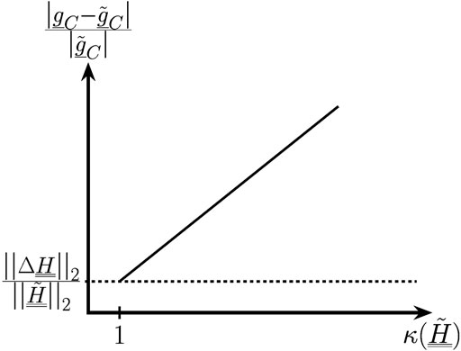
FIGURE 2. Sketch of the upper bound for the relative estimation error resulting from measurement position errors with respect to the condition number $\kappa \left(\underset{¯}{\underset{¯}{\tilde{H}}}\right)$ of the shape matrix.

3.4 Measurement Errors and Measurement Position Errors

Within the former sections the influences of measurement errors and measurement position errors have been discussed separately. Within the practical application it is expectable that both errors occur simultanously. The relative error resulting from the noisy measurements and the perturbed measurement positions is given by the quadratic sum of the two cases discussed above

$\frac{{\left|{\underset{¯}{g}}_C-{\underset{¯}{\tilde{g}}}_C\right|}^2}{{\left|{\underset{¯}{\tilde{g}}}_C\right|}^2}\le {\kappa }^2\left(\underset{¯}{\underset{¯}{\tilde{H}}}\right)\left(\frac{{\Vert \text{Δ}\underset{¯}{\underset{¯}{H}}\Vert }_2^2}{{\Vert \underset{¯}{\underset{¯}{\tilde{H}}}\Vert }_2^2}+\frac{{\left|\langle \delta \underset{¯}{B}\rangle \right|}^2}{{\left|\langle \underset{¯}{\tilde{B}}\rangle \right|}^2}\right).(58)$

This can be derived as follows:

The accurate model is given by

$\langle \underset{¯}{B}\rangle =\underset{¯}{\underset{¯}{H}}\underset{¯}{g}+\langle \underset{¯}{v}\rangle ,(59)$

so that the corresponding accurate estimator results in

${\underset{¯}{g}}_C={\underset{¯}{\underset{¯}{w}}}^{†}\langle \underset{¯}{B}\rangle (60)$

where

${\underset{¯}{\underset{¯}{w}}}^{†}={\left[{\underset{¯}{\underset{¯}{H}}}^{†}{\underset{¯}{\underset{¯}{M}}}^{-1}\underset{¯}{\underset{¯}{H}}\right]}^{-1}{\underset{¯}{\underset{¯}{H}}}^{†}{\underset{¯}{\underset{¯}{M}}}^{-1}.(61)$

The measured data are not affected by the perturbed determination of the sensor’s positions. The data are solely affected by measurement errors $\langle \delta \underset{¯}{B}\rangle$ so that the perturbed model can be written as

$\langle \underset{¯}{\tilde{B}}\rangle =\langle \underset{¯}{B}\rangle +\langle \delta \underset{¯}{B}\rangle =\underset{¯}{\underset{¯}{\tilde{H}}}\underset{¯}{\tilde{g}}+\langle \underset{¯}{\tilde{v}}\rangle +\langle \delta \underset{¯}{B}\rangle (62)$

The corresponding perturbed estimator results in

${\underset{¯}{\tilde{g}}}_C={\underset{¯}{\underset{¯}{\tilde{w}}}}^{†}\langle \underset{¯}{\tilde{B}}\rangle ,(63)$

where

${\underset{¯}{\underset{¯}{\tilde{w}}}}^{†}={\left[{\underset{¯}{\underset{¯}{\tilde{H}}}}^{†}{\underset{¯}{\underset{¯}{\tilde{M}}}}^{-1}\underset{¯}{\underset{¯}{\tilde{H}}}\right]}^{-1}{\underset{¯}{\underset{¯}{\tilde{H}}}}^{†}{\underset{¯}{\underset{¯}{\tilde{M}}}}^{-1}(64)$

and $\underset{¯}{\underset{¯}{M}}=\underset{¯}{\underset{¯}{\tilde{M}}}+\text{Δ}\underset{¯}{\underset{¯}{M}}$. The noisy shape matrix can again be written as $\underset{¯}{\underset{¯}{H}}=\underset{¯}{\underset{¯}{\tilde{H}}}+\text{Δ}\underset{¯}{\underset{¯}{H}}$ within a linear approximation. Thus, the deviation between the accurate and the perturbed estimator is given by

$\begin{array}{l}{\underset{¯}{g}}_C-{\underset{¯}{\tilde{g}}}_C={\underset{¯}{\underset{¯}{w}}}^{†}\langle \underset{¯}{B}\rangle -{\underset{¯}{\underset{¯}{\tilde{w}}}}^{†}\langle \underset{¯}{\tilde{B}}\rangle ={\underset{¯}{\underset{¯}{w}}}^{†}\langle \underset{¯}{\tilde{B}}\rangle -{\underset{¯}{\underset{¯}{w}}}^{†}\langle \delta \underset{¯}{B}\rangle -{\underset{¯}{\underset{¯}{\tilde{w}}}}^{†}\langle \underset{¯}{\tilde{B}}\rangle \\ =\left({\underset{¯}{\underset{¯}{w}}}^{†}-{\underset{¯}{\underset{¯}{\tilde{w}}}}^{†}\right)\langle \underset{¯}{\tilde{B}}\rangle -{\underset{¯}{\underset{¯}{w}}}^{†}\langle \delta \underset{¯}{B}\rangle .\end{array}(65)$

By making use of the Neumann series, the unknown filter matrix ${\underset{¯}{\underset{¯}{w}}}^{†}$ can be rewritten within a linear approximation resulting in

$\begin{array}{c}{\underset{¯}{\underset{¯}{w}}}^{†}={\left[{\underset{¯}{\underset{¯}{H}}}^{†}{\underset{¯}{\underset{¯}{M}}}^{-1}\underset{¯}{\underset{¯}{H}}\right]}^{-1}{\underset{¯}{\underset{¯}{H}}}^{†}{\underset{¯}{\underset{¯}{M}}}^{-1}\\ ={\left[\left({\underset{¯}{\underset{¯}{\tilde{H}}}}^{†}+\text{Δ}{\underset{¯}{\underset{¯}{H}}}^{†}\right){\left(\underset{¯}{\underset{¯}{\tilde{M}}}+\text{Δ}\underset{¯}{\underset{¯}{M}}\right)}^{-1}\left(\underset{¯}{\underset{¯}{\tilde{H}}}+\text{Δ}\underset{¯}{\underset{¯}{H}}\right)\right]}^{-1}\left({\underset{¯}{\underset{¯}{\tilde{H}}}}^{†}+\text{Δ}{\underset{¯}{\underset{¯}{H}}}^{†}\right){\left(\underset{¯}{\underset{¯}{\tilde{M}}}+\text{Δ}\underset{¯}{\underset{¯}{M}}\right)}^{-1}\\ ={\left[\left({\underset{¯}{\underset{¯}{\tilde{H}}}}^{†}+\text{Δ}{\underset{¯}{\underset{¯}{H}}}^{†}\right)\left({\underset{¯}{\underset{¯}{\tilde{M}}}}^{-1}-{\underset{¯}{\underset{¯}{\tilde{M}}}}^{-1}\text{Δ}\underset{¯}{\underset{¯}{M}}{\underset{¯}{\underset{¯}{\tilde{M}}}}^{-1}\right)\left(\underset{¯}{\underset{¯}{\tilde{H}}}+\text{Δ}\underset{¯}{\underset{¯}{H}}\right)\right]}^{-1}\left({\underset{¯}{\underset{¯}{\tilde{H}}}}^{†}+\text{Δ}{\underset{¯}{\underset{¯}{H}}}^{†}\right)\left({\underset{¯}{\underset{¯}{\tilde{M}}}}^{-1}-{\underset{¯}{\underset{¯}{\tilde{M}}}}^{-1}\text{Δ}\underset{¯}{\underset{¯}{M}}{\underset{¯}{\underset{¯}{\tilde{M}}}}^{-1}\right).\end{array}$

Using

$\begin{array}{l}\left({\underset{¯}{\underset{¯}{\tilde{H}}}}^{†}+\text{Δ}{\underset{¯}{\underset{¯}{H}}}^{†}\right)\left({\underset{¯}{\underset{¯}{\tilde{M}}}}^{-1}-{\underset{¯}{\underset{¯}{\tilde{M}}}}^{-1}\text{Δ}\underset{¯}{\underset{¯}{M}}{\underset{¯}{\underset{¯}{\tilde{M}}}}^{-1}\right)\left(\underset{¯}{\underset{¯}{\tilde{H}}}+\text{Δ}\underset{¯}{\underset{¯}{H}}\right)\\ =\left({\underset{¯}{\underset{¯}{\tilde{H}}}}^{†}{\underset{¯}{\underset{¯}{\tilde{M}}}}^{-1}-{\underset{¯}{\underset{¯}{\tilde{H}}}}^{†}{\underset{¯}{\underset{¯}{\tilde{M}}}}^{-1}\text{Δ}\underset{¯}{\underset{¯}{M}}{\underset{¯}{\underset{¯}{\tilde{M}}}}^{-1}+\text{Δ}{\underset{¯}{\underset{¯}{H}}}^{†}{\underset{¯}{\underset{¯}{\tilde{M}}}}^{-1}\right)\left(\underset{¯}{\underset{¯}{\tilde{H}}}+\text{Δ}\underset{¯}{\underset{¯}{H}}\right)\\ ={\underset{¯}{\underset{¯}{\tilde{H}}}}^{†}{\underset{¯}{\underset{¯}{\tilde{M}}}}^{-1}\underset{¯}{\underset{¯}{\tilde{H}}}-{\underset{¯}{\underset{¯}{\tilde{H}}}}^{†}{\underset{¯}{\underset{¯}{\tilde{M}}}}^{-1}\text{Δ}\underset{¯}{\underset{¯}{M}}{\underset{¯}{\underset{¯}{\tilde{M}}}}^{-1}\underset{¯}{\underset{¯}{\tilde{H}}}+\text{Δ}{\underset{¯}{\underset{¯}{H}}}^{†}{\underset{¯}{\underset{¯}{\tilde{M}}}}^{-1}\underset{¯}{\underset{¯}{\tilde{H}}}+{\underset{¯}{\underset{¯}{\tilde{H}}}}^{†}{\underset{¯}{\underset{¯}{\tilde{M}}}}^{-1}\text{Δ}\underset{¯}{\underset{¯}{H}}\\ ={\underset{¯}{\underset{¯}{\tilde{P}}}}^{-1}-{\underset{¯}{\underset{¯}{\tilde{H}}}}^{†}{\underset{¯}{\underset{¯}{\tilde{M}}}}^{-1}\text{Δ}\underset{¯}{\underset{¯}{M}}{\underset{¯}{\underset{¯}{\tilde{M}}}}^{-1}\underset{¯}{\underset{¯}{\tilde{H}}}+\text{Δ}{\underset{¯}{\underset{¯}{H}}}^{†}{\underset{¯}{\underset{¯}{\tilde{M}}}}^{-1}\underset{¯}{\underset{¯}{\tilde{H}}}+{\underset{¯}{\underset{¯}{\tilde{H}}}}^{†}{\underset{¯}{\underset{¯}{\tilde{M}}}}^{-1}\text{Δ}\underset{¯}{\underset{¯}{H}}\end{array}(66)$

and again making use of the Neumann series delivers

$\begin{array}{l}{\underset{¯}{\underset{¯}{w}}}^{†}=\left[\underset{¯}{\underset{¯}{\tilde{P}}}+\underset{¯}{\underset{¯}{\tilde{P}}}{\underset{¯}{\underset{¯}{\tilde{H}}}}^{†}{\underset{¯}{\underset{¯}{\tilde{M}}}}^{-1}\text{Δ}\underset{¯}{\underset{¯}{M}}{\underset{¯}{\underset{¯}{\tilde{M}}}}^{-1}\underset{¯}{\underset{¯}{\tilde{H}}}\underset{¯}{\underset{¯}{\tilde{P}}}-\underset{¯}{\underset{¯}{\tilde{P}}}\text{Δ}{\underset{¯}{\underset{¯}{H}}}^{†}{\underset{¯}{\underset{¯}{\tilde{M}}}}^{-1}\underset{¯}{\underset{¯}{\tilde{H}}}\underset{¯}{\underset{¯}{\tilde{P}}}-\underset{¯}{\underset{¯}{\tilde{P}}}{\underset{¯}{\underset{¯}{\tilde{H}}}}^{†}{\underset{¯}{\underset{¯}{\tilde{M}}}}^{-1}\text{Δ}\underset{¯}{\underset{¯}{H}}\underset{¯}{\underset{¯}{\tilde{P}}}\right]\\ \cdot \left({\underset{¯}{\underset{¯}{\tilde{H}}}}^{†}{\underset{¯}{\underset{¯}{\tilde{M}}}}^{-1}-{\underset{¯}{\underset{¯}{\tilde{H}}}}^{†}{\underset{¯}{\underset{¯}{\tilde{M}}}}^{-1}\text{Δ}\underset{¯}{\underset{¯}{M}}{\underset{¯}{\underset{¯}{\tilde{M}}}}^{-1}+\text{Δ}{\underset{¯}{\underset{¯}{H}}}^{†}{\underset{¯}{\underset{¯}{\tilde{M}}}}^{-1}\right)\\ =\underset{¯}{\underset{¯}{\tilde{P}}}{\underset{¯}{\underset{¯}{\tilde{H}}}}^{†}{\underset{¯}{\underset{¯}{\tilde{M}}}}^{-1}-\underset{¯}{\underset{¯}{\tilde{P}}}{\underset{¯}{\underset{¯}{\tilde{H}}}}^{†}{\underset{¯}{\underset{¯}{\tilde{M}}}}^{-1}\text{Δ}\underset{¯}{\underset{¯}{M}}{\underset{¯}{\underset{¯}{\tilde{M}}}}^{-1}+\underset{¯}{\underset{¯}{\tilde{P}}}\text{Δ}{\underset{¯}{\underset{¯}{H}}}^{†}{\underset{¯}{\underset{¯}{\tilde{M}}}}^{-1}\\ +\underset{¯}{\underset{¯}{\tilde{P}}}{\underset{¯}{\underset{¯}{\tilde{H}}}}^{†}{\underset{¯}{\underset{¯}{\tilde{M}}}}^{-1}\text{Δ}\underset{¯}{\underset{¯}{M}}{\underset{¯}{\underset{¯}{\tilde{M}}}}^{-1}\underset{¯}{\underset{¯}{\tilde{H}}}\underset{¯}{\underset{¯}{\tilde{P}}}{\underset{¯}{\underset{¯}{\tilde{H}}}}^{†}{\underset{¯}{\underset{¯}{\tilde{M}}}}^{-1}-\underset{¯}{\underset{¯}{\tilde{P}}}\text{Δ}{\underset{¯}{\underset{¯}{H}}}^{†}{\underset{¯}{\underset{¯}{\tilde{M}}}}^{-1}\underset{¯}{\underset{¯}{\tilde{H}}}\underset{¯}{\underset{¯}{\tilde{P}}}{\underset{¯}{\underset{¯}{\tilde{H}}}}^{†}{\underset{¯}{\underset{¯}{\tilde{M}}}}^{-1}\\ -\underset{¯}{\underset{¯}{\tilde{P}}}{\underset{¯}{\underset{¯}{\tilde{H}}}}^{†}{\underset{¯}{\underset{¯}{\tilde{M}}}}^{-1}\text{Δ}\underset{¯}{\underset{¯}{H}}\underset{¯}{\underset{¯}{\tilde{P}}}{\underset{¯}{\underset{¯}{\tilde{H}}}}^{†}{\underset{¯}{\underset{¯}{\tilde{M}}}}^{-1}={\underset{¯}{\underset{¯}{\tilde{w}}}}^{†}-{\underset{¯}{\underset{¯}{\tilde{w}}}}^{†}\text{Δ}\underset{¯}{\underset{¯}{M}}{\underset{¯}{\underset{¯}{\tilde{M}}}}^{-1}+\underset{¯}{\underset{¯}{\tilde{P}}}\text{Δ}{\underset{¯}{\underset{¯}{H}}}^{†}{\underset{¯}{\underset{¯}{\tilde{M}}}}^{-1}\\ +{\underset{¯}{\underset{¯}{\tilde{w}}}}^{†}\text{Δ}\underset{¯}{\underset{¯}{M}}{\underset{¯}{\underset{¯}{\tilde{M}}}}^{-1}\underset{¯}{\underset{¯}{\tilde{H}}}{\underset{¯}{\underset{¯}{\tilde{w}}}}^{†}-\underset{¯}{\underset{¯}{\tilde{P}}}\text{Δ}{\underset{¯}{\underset{¯}{H}}}^{†}{\underset{¯}{\underset{¯}{\tilde{M}}}}^{-1}\underset{¯}{\underset{¯}{\tilde{H}}}{\underset{¯}{\underset{¯}{\tilde{w}}}}^{†}-{\underset{¯}{\underset{¯}{\tilde{w}}}}^{†}\text{Δ}\underset{¯}{\underset{¯}{H}}{\underset{¯}{\underset{¯}{\tilde{w}}}}^{†}.\end{array}(67)$

Taking into account that

${\underset{¯}{\underset{¯}{w}}}^{†}\langle \delta \underset{¯}{B}\rangle ={\underset{¯}{\underset{¯}{\tilde{w}}}}^{†}\langle \delta \underset{¯}{B}\rangle (68)$

within the linear approximation as well as

$\begin{array}{l}{\underset{¯}{\underset{¯}{w}}}^{†}-{\underset{¯}{\underset{¯}{\tilde{w}}}}^{†}=-{\underset{¯}{\underset{¯}{\tilde{w}}}}^{†}\text{Δ}\underset{¯}{\underset{¯}{M}}{\underset{¯}{\underset{¯}{\tilde{M}}}}^{-1}+\underset{¯}{\underset{¯}{\tilde{P}}}\text{Δ}{\underset{¯}{\underset{¯}{H}}}^{†}{\underset{¯}{\underset{¯}{\tilde{M}}}}^{-1}+{\underset{¯}{\underset{¯}{\tilde{w}}}}^{†}\text{Δ}\underset{¯}{\underset{¯}{M}}{\underset{¯}{\underset{¯}{\tilde{M}}}}^{-1}\underset{¯}{\underset{¯}{\tilde{H}}}{\underset{¯}{\underset{¯}{\tilde{w}}}}^{†}\\ -\underset{¯}{\underset{¯}{\tilde{P}}}\text{Δ}{\underset{¯}{\underset{¯}{H}}}^{†}{\underset{¯}{\underset{¯}{\tilde{M}}}}^{-1}\underset{¯}{\underset{¯}{\tilde{H}}}{\underset{¯}{\underset{¯}{\tilde{w}}}}^{†}-{\underset{¯}{\underset{¯}{\tilde{w}}}}^{†}\text{Δ}\underset{¯}{\underset{¯}{H}}{\underset{¯}{\underset{¯}{\tilde{w}}}}^{†},\end{array}(69)$

the deviation between the estimators can be approximated by

$\begin{array}{l}{\underset{¯}{g}}_C-{\underset{¯}{\tilde{g}}}_C=\left({\underset{¯}{\underset{¯}{w}}}^{†}-{\underset{¯}{\underset{¯}{\tilde{w}}}}^{†}\right)\langle \underset{¯}{\tilde{B}}\rangle -{\underset{¯}{\underset{¯}{w}}}^{†}\langle \delta \underset{¯}{B}\rangle \\ =-{\underset{¯}{\underset{¯}{\tilde{w}}}}^{†}\text{Δ}\underset{¯}{\underset{¯}{M}}{\underset{¯}{\underset{¯}{\tilde{M}}}}^{-1}\langle \underset{¯}{\tilde{B}}\rangle +\underset{¯}{\underset{¯}{\tilde{P}}}\text{Δ}{\underset{¯}{\underset{¯}{H}}}^{†}{\underset{¯}{\underset{¯}{\tilde{M}}}}^{-1}\langle \underset{¯}{\tilde{B}}\rangle +{\underset{¯}{\underset{¯}{\tilde{w}}}}^{†}\text{Δ}\underset{¯}{\underset{¯}{M}}{\underset{¯}{\underset{¯}{\tilde{M}}}}^{-1}\underset{¯}{\underset{¯}{\tilde{H}}}{\underset{¯}{\underset{¯}{\tilde{w}}}}^{†}\langle \underset{¯}{\tilde{B}}\rangle \\ -\underset{¯}{\underset{¯}{\tilde{P}}}\text{Δ}{\underset{¯}{\underset{¯}{H}}}^{†}{\underset{¯}{\underset{¯}{\tilde{M}}}}^{-1}\underset{¯}{\underset{¯}{\tilde{H}}}{\underset{¯}{\underset{¯}{\tilde{w}}}}^{†}\langle \underset{¯}{\tilde{B}}\rangle -{\underset{¯}{\underset{¯}{\tilde{w}}}}^{†}\text{Δ}\underset{¯}{\underset{¯}{H}}{\underset{¯}{\underset{¯}{\tilde{w}}}}^{†}\langle \underset{¯}{\tilde{B}}\rangle -{\underset{¯}{\underset{¯}{\tilde{w}}}}^{†}\langle \delta \underset{¯}{B}\rangle \end{array}(70)$

Using ${\underset{¯}{\underset{¯}{\tilde{w}}}}^{†}\langle \underset{¯}{\tilde{B}}\rangle ={\underset{¯}{\tilde{g}}}_C$, it follows that

$\begin{array}{l}{\underset{¯}{g}}_C-{\underset{¯}{\tilde{g}}}_C=-{\underset{¯}{\underset{¯}{\tilde{w}}}}^{†}\text{Δ}\underset{¯}{\underset{¯}{M}}{\underset{¯}{\underset{¯}{\tilde{M}}}}^{-1}\langle \underset{¯}{\tilde{B}}\rangle +\underset{¯}{\underset{¯}{\tilde{P}}}\text{Δ}{\underset{¯}{\underset{¯}{H}}}^{†}{\underset{¯}{\underset{¯}{\tilde{M}}}}^{-1}\langle \underset{¯}{\tilde{B}}\rangle +{\underset{¯}{\underset{¯}{\tilde{w}}}}^{†}\text{Δ}\underset{¯}{\underset{¯}{M}}{\underset{¯}{\underset{¯}{\tilde{M}}}}^{-1}\underset{¯}{\underset{¯}{\tilde{H}}}{\underset{¯}{\tilde{g}}}_C\\ -\underset{¯}{\underset{¯}{\tilde{P}}}\text{Δ}{\underset{¯}{\underset{¯}{H}}}^{†}{\underset{¯}{\underset{¯}{\tilde{M}}}}^{-1}\underset{¯}{\underset{¯}{\tilde{H}}}{\underset{¯}{\tilde{g}}}_C-{\underset{¯}{\underset{¯}{\tilde{w}}}}^{†}\text{Δ}\underset{¯}{\underset{¯}{H}}{\underset{¯}{\tilde{g}}}_C-{\underset{¯}{\underset{¯}{\tilde{w}}}}^{†}\langle \delta \underset{¯}{B}\rangle \\ ={\underset{¯}{\underset{¯}{\tilde{w}}}}^{†}\text{Δ}\underset{¯}{\underset{¯}{M}}{\underset{¯}{\underset{¯}{\tilde{M}}}}^{-1}\left(\underset{¯}{\underset{¯}{\tilde{H}}}{\underset{¯}{\tilde{g}}}_C-\langle \underset{¯}{\tilde{B}}\rangle \right)+\underset{¯}{\underset{¯}{\tilde{P}}}\text{Δ}{\underset{¯}{\underset{¯}{H}}}^{†}{\underset{¯}{\underset{¯}{\tilde{M}}}}^{-1}\left(\langle \underset{¯}{\tilde{B}}\rangle -\underset{¯}{\underset{¯}{\tilde{H}}}{\underset{¯}{\tilde{g}}}_C\right)\\ -{\underset{¯}{\underset{¯}{\tilde{w}}}}^{†}\text{Δ}\underset{¯}{\underset{¯}{H}}{\underset{¯}{\tilde{g}}}_C-{\underset{¯}{\underset{¯}{\tilde{w}}}}^{†}\langle \delta \underset{¯}{B}\rangle \end{array}(71)$

and thus,

$\begin{array}{l}{\left|{\underset{¯}{g}}_C-{\underset{¯}{\tilde{g}}}_C\right|}^2={\Vert {\underset{¯}{\underset{¯}{\tilde{w}}}}^{†}\text{Δ}\underset{¯}{\underset{¯}{M}}{\underset{¯}{\underset{¯}{\tilde{M}}}}^{-1/2}{\underset{¯}{\underset{¯}{\tilde{M}}}}^{-1/2}\left(\underset{¯}{\underset{¯}{\tilde{H}}}{\underset{¯}{\tilde{g}}}_C-\langle \underset{¯}{\tilde{B}}\rangle \right)+\underset{¯}{\underset{¯}{\tilde{P}}}\text{Δ}{\underset{¯}{\underset{¯}{H}}}^{†}{\underset{¯}{\underset{¯}{\tilde{M}}}}^{-1/2}{\underset{¯}{\underset{¯}{\tilde{M}}}}^{-1/2}\left(\langle \underset{¯}{\tilde{B}}\rangle -\underset{¯}{\underset{¯}{\tilde{H}}}{\underset{¯}{\tilde{g}}}_C\right)-{\underset{¯}{\underset{¯}{\tilde{w}}}}^{†}\text{Δ}\underset{¯}{\underset{¯}{H}}{\underset{¯}{\tilde{g}}}_C-{\underset{¯}{\underset{¯}{\tilde{w}}}}^{†}\langle \delta \underset{¯}{B}\rangle \Vert }_2^2\\ \le {\Vert {\underset{¯}{\underset{¯}{\tilde{w}}}}^{†}\text{Δ}\underset{¯}{\underset{¯}{M}}{\underset{¯}{\underset{¯}{\tilde{M}}}}^{-1/2}\Vert }_2^2\cdot {\left|{\underset{¯}{\underset{¯}{\tilde{M}}}}^{-1/2}\left(\underset{¯}{\underset{¯}{\tilde{H}}}{\underset{¯}{\tilde{g}}}_C-\langle \underset{¯}{\tilde{B}}\rangle \right)\right|}^2+{\Vert \underset{¯}{\underset{¯}{\tilde{P}}}\text{Δ}{\underset{¯}{\underset{¯}{H}}}^{†}{\underset{¯}{\underset{¯}{\tilde{M}}}}^{-1/2}\Vert }_2^2\cdot {\left|{\underset{¯}{\underset{¯}{\tilde{M}}}}^{-1/2}\left(\langle \underset{¯}{\tilde{B}}\rangle -\underset{¯}{\underset{¯}{\tilde{H}}}{\underset{¯}{\tilde{g}}}_C\right)\right|}^2\\ +{\Vert {\underset{¯}{\underset{¯}{\tilde{w}}}}^{†}\Vert }_2^2\cdot {\Vert \text{Δ}\underset{¯}{\underset{¯}{H}}\Vert }_2^2\cdot {\left|{\underset{¯}{\tilde{g}}}_C\right|}^2+{\Vert {\underset{¯}{\underset{¯}{\tilde{w}}}}^{†}\Vert }_2^2\cdot {\left|\langle \delta \underset{¯}{B}\rangle \right|}^2\to {\Vert {\underset{¯}{\underset{¯}{\tilde{w}}}}^{†}\Vert }_2^2\cdot {\Vert \text{Δ}\underset{¯}{\underset{¯}{H}}\Vert }_2^2\cdot {\left|{\underset{¯}{\tilde{g}}}_C\right|}^2+{\Vert {\underset{¯}{\underset{¯}{\tilde{w}}}}^{†}\Vert }_2^2\cdot {\left|\langle \delta \underset{¯}{B}\rangle \right|}^2.\end{array}(72)$

Assuming that $\langle \underset{¯}{\tilde{B}}\rangle \approx \underset{¯}{\underset{¯}{\tilde{H}}}{\underset{¯}{\tilde{g}}}_C$ the relative error can be estimated by

$\begin{array}{l}\frac{{\left|{\underset{¯}{g}}_C-{\underset{¯}{\tilde{g}}}_C\right|}^2}{{\left|{\underset{¯}{\tilde{g}}}_C\right|}^2}={\Vert {\underset{¯}{\underset{¯}{\tilde{w}}}}^{†}\Vert }_2^2\cdot {\Vert \text{Δ}\underset{¯}{\underset{¯}{H}}\Vert }_2^2+{\Vert {\underset{¯}{\underset{¯}{\tilde{w}}}}^{†}\Vert }_2^2\cdot \frac{{\left|\langle \delta \underset{¯}{B}\rangle \right|}^2}{{\left|\langle \underset{¯}{\tilde{B}}\rangle \right|}^2}\frac{{\left|\langle \underset{¯}{\tilde{B}}\rangle \right|}^2}{{\left|{\underset{¯}{\tilde{g}}}_C\right|}^2}\\ ={\Vert {\underset{¯}{\underset{¯}{\tilde{w}}}}^{†}\Vert }_2^2\cdot {\Vert \underset{¯}{\underset{¯}{\tilde{H}}}\Vert }_2^2\cdot \frac{{\Vert \text{Δ}\underset{¯}{\underset{¯}{H}}\Vert }_2^2}{{\Vert \underset{¯}{\underset{¯}{\tilde{H}}}\Vert }_2^2}+{\Vert {\underset{¯}{\underset{¯}{\tilde{w}}}}^{†}\Vert }_2^2\cdot \frac{{\left|\langle \delta \underset{¯}{B}\rangle \right|}^2}{{\left|\langle \underset{¯}{\tilde{B}}\rangle \right|}^2}\frac{{\left|\underset{¯}{\underset{¯}{\tilde{H}}}{\underset{¯}{\tilde{g}}}_C\right|}^2}{{\left|{\underset{¯}{\tilde{g}}}_C\right|}^2}\\ \le {\Vert {\underset{¯}{\underset{¯}{\tilde{w}}}}^{†}\Vert }_2^2\cdot {\Vert \underset{¯}{\underset{¯}{\tilde{H}}}\Vert }_2^2\cdot \frac{{\Vert \text{Δ}\underset{¯}{\underset{¯}{H}}\Vert }_2^2}{{\Vert \underset{¯}{\underset{¯}{\tilde{H}}}\Vert }_2^2}+{\Vert {\underset{¯}{\underset{¯}{\tilde{w}}}}^{†}\Vert }_2^2\cdot {\left|\right|\underset{¯}{\underset{¯}{\tilde{H}}}\left|\right|}_2^2\cdot \frac{{\left|\langle \delta \underset{¯}{B}\rangle \right|}^2}{{\left|\langle \underset{¯}{\tilde{B}}\rangle \right|}^2}\\ ={\Vert {\underset{¯}{\underset{¯}{\tilde{w}}}}^{†}\Vert }_2^2\cdot {\Vert \underset{¯}{\underset{¯}{\tilde{H}}}\Vert }_2^2\cdot \left(\frac{{\Vert \text{Δ}\underset{¯}{\underset{¯}{H}}\Vert }_2^2}{{\Vert \underset{¯}{\underset{¯}{\tilde{H}}}\Vert }_2^2}+\frac{{\left|\langle \delta \underset{¯}{B}\rangle \right|}^2}{{\left|\langle \underset{¯}{\tilde{B}}\rangle \right|}^2}\right)\\ ={\kappa }^2\left(\underset{¯}{\underset{¯}{\tilde{H}}}\right)\left(\frac{{\Vert \text{Δ}\underset{¯}{\underset{¯}{H}}\Vert }_2^2}{{\Vert \underset{¯}{\underset{¯}{\tilde{H}}}\Vert }_2^2}+\frac{{\left|\langle \delta \underset{¯}{B}\rangle \right|}^2}{{\left|\langle \underset{¯}{\tilde{B}}\rangle \right|}^2}\right)\end{array}(73)$

It is important to note that the right sides of Eqs. 35, 56 and 73 represent upper bounds for the error of the estimator. These bounds can be much larger than the true errors. The great advantage of the bounds lies in the fact that they solely depend on known quantities, wheras the accurate estimator for calculating the true estimation error is unknown within the practical application of the method. Thus, the above derived upper bounds are conservative and guarantee that the true estimation errors cannot exceed these bounds as long as the measurement errors as well as the measurement position errors are much smaller than the measurements themselves so that the linear approximation is valid.

4 Finite Sample Averaging

For the calculation of Capon’s estimator, averaged magnetic field data

$\langle \underset{¯}{B}\rangle =\frac{1}{Q}{\displaystyle \sum }_{\alpha =1}^Q{\underset{¯}{B}}^{\alpha }(74)$

are required [3]. Here, Q denotes the number of measurements at a fixed set of data points. Within the practical application of the method only a finite number $Q<\infty$ of samples is available, which yields a standard deviation of Capon’s estimator ${\underset{¯}{g}}_C$. In the following, an approximation for the variance of Capon’s estimator is derived by regarding Capon’s method as a special case of the maximum likelihood method [6].

In the vicinity of its maximum value the likelihood function can be approximated as

$\mathrm{ℒ}\sim \text{exp}\left[-\frac{1}{2}{\displaystyle \sum }_{\alpha =1}^Q{\left({\underset{¯}{B}}^{\alpha }-\underset{¯}{\underset{¯}{H}}\underset{¯}{g}\right)}^{†}{\underset{¯}{\underset{¯}{N}}}^{-1}\left({\underset{¯}{B}}^{\alpha }-\underset{¯}{\underset{¯}{H}}\underset{¯}{g}\right)\right],(75)$

where $\underset{¯}{\underset{¯}{N}}$ denotes the noise covariance matrix [6, 19]. Before deducing the error resulting from the finite number of samples let us make a general comment about the construction of the likelihood function in terms of the averaging process. The noise matrix is already statistically evaluated so that the likelihood function is constructed by making use of two different averaging processes. Within the first averaging process the noise matrix $\underset{¯}{\underset{¯}{N}}$ is calculated. This averaging process does not incorporate the underlying model since only the distribution of the data around the mean value $\langle \underset{¯}{B}\rangle$ is determined which allows to assess the general quality of the measurements. When the distribution of the measurements is large, significant errors within the subsequent data fitting are expectable. Especially, these errors are independent of the chosen model. Within the second averaging process a specific underlying model $\underset{¯}{\underset{¯}{H}}\underset{¯}{g}$ is fitted to the data ${\underset{¯}{B}}^{\alpha }$.

For most practical applications, the noise matrix $\underset{¯}{\underset{¯}{N}}$ is unknown and has to be approximated. In the special case of Gaussian errors with zero mean and variance ${\sigma }_n$, the noise covariance matrix can be written as $\underset{¯}{\underset{¯}{N}}={\sigma }_n^2\underset{¯}{\underset{¯}{I}}$, where $\underset{¯}{\underset{¯}{I}}$ denotes the identity matrix. Substituting the noise covariance matrix $\underset{¯}{\underset{¯}{N}}$ by the data covariance matrix $\underset{¯}{\underset{¯}{M}}=\langle \underset{¯}{B}\circ \underset{¯}{B}\rangle$, the maximum likelihood estimator may be converted into Capon’s estimator [6]. The corresponding likelihood function is modified to

$\mathrm{ℒ}\sim \text{exp}\left[-\frac{1}{2}{\displaystyle \sum }_{\alpha =1}^Q{\left({\underset{¯}{B}}^{\alpha }-\underset{¯}{\underset{¯}{H}}\underset{¯}{g}\right)}^{†}{\underset{¯}{\underset{¯}{M}}}^{-1}\left({\underset{¯}{B}}^{\alpha }-\underset{¯}{\underset{¯}{H}}\underset{¯}{g}\right)\right].(76)$

The weighted difference between the model and the data can be rewritten as

$\begin{array}{l}{\left({\underset{¯}{B}}^{\alpha }-\underset{¯}{\underset{¯}{H}}\underset{¯}{g}\right)}^{†}{\underset{¯}{\underset{¯}{M}}}^{-1}\left({\underset{¯}{B}}^{\alpha }-\underset{¯}{\underset{¯}{H}}\underset{¯}{g}\right)=\left({\underset{¯}{B}}^{\alpha †}-{\underset{¯}{g}}^{†}{\underset{¯}{\underset{¯}{H}}}^{†}\right){\underset{¯}{\underset{¯}{M}}}^{-1}\left({\underset{¯}{B}}^{\alpha }-\underset{¯}{\underset{¯}{H}}\underset{¯}{g}\right)\\ ={\underset{¯}{B}}^{\alpha †}{\underset{¯}{\underset{¯}{M}}}^{-1}{\underset{¯}{B}}^{\alpha }-2{\underset{¯}{g}}^{†}{\underset{¯}{\underset{¯}{H}}}^{†}{\underset{¯}{\underset{¯}{M}}}^{-1}{\underset{¯}{B}}^{\alpha }+{\underset{¯}{g}}^{†}{\underset{¯}{\underset{¯}{H}}}^{†}{\underset{¯}{\underset{¯}{M}}}^{-1}\underset{¯}{\underset{¯}{H}}\underset{¯}{g}.\end{array}(77)$

As discussed above, the data covariance matrix $\underset{¯}{\underset{¯}{M}}$ is already statistically evaluated so that the averaging process results in

${\displaystyle \sum }_{\alpha =1}^Q{\left({\underset{¯}{B}}^{\alpha }-\underset{¯}{\underset{¯}{H}}\underset{¯}{g}\right)}^{†}{\underset{¯}{\underset{¯}{M}}}^{-1}\left({\underset{¯}{B}}^{\alpha }-\underset{¯}{\underset{¯}{H}}\underset{¯}{g}\right)=Q\langle {\underset{¯}{B}}^{†}{\underset{¯}{\underset{¯}{M}}}^{-1}\underset{¯}{B}\rangle -2Q{\underset{¯}{g}}^{†}{\underset{¯}{\underset{¯}{H}}}^{†}{\underset{¯}{\underset{¯}{M}}}^{-1}\langle \underset{¯}{B}\rangle +Q{\underset{¯}{g}}^{†}{\underset{¯}{\underset{¯}{H}}}^{†}{\underset{¯}{\underset{¯}{M}}}^{-1}\underset{¯}{\underset{¯}{H}}\underset{¯}{g}.(78)$

Insertion into Eq. 76 yields

$\mathrm{ℒ}\sim \text{exp}\left\{-\frac{Q}{2}[\langle {\underset{¯}{B}}^{†}{\underset{¯}{\underset{¯}{M}}}^{-1}\underset{¯}{B}\rangle -2{\underset{¯}{g}}^{†}{\underset{¯}{\underset{¯}{H}}}^{†}{\underset{¯}{\underset{¯}{M}}}^{-1}\langle \underset{¯}{B}\rangle +{\underset{¯}{g}}^{†}{\underset{¯}{\underset{¯}{H}}}^{†}{\underset{¯}{\underset{¯}{M}}}^{-1}\underset{¯}{\underset{¯}{H}}\underset{¯}{g}]\right\}(79)$

or equivalently

$\mathrm{ℒ}\sim \text{exp}\left\{-\frac{Q}{2}\left[\langle B_i{M}_{ij}^{-1}{B}_j\rangle -2g_k{H}_{ki}^{†}{M}_{ij}^{-1}\langle B_j\rangle +g_l{H}_{lk}^{†}{M}_{ki}^{-1}{H}_{ij}{g}_j\right]\right\}.(80)$

The m’th component of Capon’s estimator ${\underset{¯}{g}}_C$ corresponds with the maximum value of the likelihood function [6, 19]. The corresponding standard deviation ($1\sigma$-error) is described by the width of the likelihood function at its maximum value which is given by [6, 19].

${\sigma }_{g_m}={[-{\partial }_{g_m}^2\text{ln}\mathrm{ℒ}]}^{-1/2},(81)$

where

${\partial }_{g_m}^2\text{ln}\mathrm{ℒ}={\partial }_{g_m}\left(\frac{1}{\mathrm{ℒ}}{\partial }_{g_m}\mathrm{ℒ}\right).(82)$

Since

$\begin{array}{l}{\partial }_{g_m}\mathrm{ℒ}=-\frac{Q}{2}\mathrm{ℒ}{\partial }_{g_m}\left[\langle B_i{M}_{ij}^{-1}{B}_j\rangle -2g_k{H}_{ki}^{†}{M}_{ij}^{-1}\langle B_j\rangle +g_l{H}_{lk}^{†}{M}_{ki}^{-1}{H}_{ij}{g}_j\right]\\ =-\frac{Q}{2}\mathrm{ℒ}\left[-2{\delta }_{km}{H}_{ki}^{†}{M}_{ij}^{-1}\langle B_j\rangle +{\delta }_{lm}{H}_{lk}^{†}{M}_{ki}^{-1}{H}_{ij}{g}_j+g_l{H}_{lk}^{†}{M}_{ki}^{-1}{H}_{ij}{\delta }_{jm}\right]\\ =-\frac{Q}{2}\mathrm{ℒ}\left[-2H_{mi}^{†}{M}_{ij}^{-1}\langle B_j\rangle +H_{mk}^{†}{M}_{ki}^{-1}{H}_{ij}{g}_j+g_l{H}_{lk}^{†}{M}_{ki}^{-1}{H}_{im}\right]\end{array}(83)$

where ${\delta }_{ij}$ denotes the Kronecker delta, the m’th component of Capon’s estimator ${\underset{¯}{g}}_C$ can be calculated via [6].

${\partial }_{g_m}\mathrm{ℒ}=0(84)$

yielding

$-2H_{mi}^{†}{M}_{ij}^{-1}\langle B_j\rangle +H_{mk}^{†}{M}_{ki}^{-1}{H}_{ij}{g}_j+g_l{H}_{lk}^{†}{M}_{ki}^{-1}{H}_{im}=0.(85)$

Because of $M_{ki}^{-1}=M_{ik}^{-1}$, as well as $H_{lk}^{†}=H_{kl}$ and $H_{im}=H_{mi}^{†}$ in the case of real shape matrices [3], it follows that

$\begin{array}{l}\text{0}=-2H_{mi}^{†}{M}_{ij}^{-1}\langle B_j\rangle +H_{mk}^{†}{M}_{ki}^{-1}{H}_{ij}{g}_j+g_l{H}_{kl}{M}_{ik}^{-1}{H}_{mi}^{†}\\ =-2H_{mi}^{†}{M}_{ij}^{-1}\langle B_j\rangle +H_{mk}^{†}{M}_{ki}^{-1}{H}_{ij}{g}_j+H_{mi}^{†}{M}_{ik}^{-1}{H}_{kl}{g}_l\\ =-2H_{mi}^{†}{M}_{ij}^{-1}\langle B_j\rangle +2H_{mk}^{†}{M}_{ki}^{-1}{H}_{ij}{g}_j\end{array}(86)$

and therefore,

${\underset{¯}{g}}_C={\left[{\underset{¯}{\underset{¯}{H}}}^{†}{\underset{¯}{\underset{¯}{M}}}^{-1}\underset{¯}{\underset{¯}{H}}\right]}^{-1}{\underset{¯}{\underset{¯}{H}}}^{†}{\underset{¯}{\underset{¯}{M}}}^{-1}\langle \underset{¯}{B}\rangle (87)$

which is in agreement with the estimator resulting from the linear algebraic formulation of Capon’s method [3]. The second derivative results in

$\begin{array}{c}{\partial }_{g_m}^2\text{ln}\mathrm{ℒ}=-\frac{Q}{2}{\partial }_{g_m}\left[-2H_{mi}^{†}{M}_{ij}^{-1}\langle B_j\rangle +H_{mk}^{†}{M}_{ki}^{-1}{H}_{ij}{g}_j+g_l{H}_{lk}^{†}{M}_{ki}^{-1}{H}_{im}\right]\\ =-\frac{Q}{2}\left[H_{mk}^{†}{M}_{ki}^{-1}{H}_{ij}{\delta }_{jm}+{\delta }_{lm}{H}_{lk}^{†}{M}_{ki}^{-1}{H}_{im}\right]\\ =-\frac{Q}{2}\left[H_{mk}^{†}{M}_{ki}^{-1}{H}_{im}+H_{mk}^{†}{M}_{ki}^{-1}{H}_{im}\right]\\ =-Q{H}_{mk}^{†}{M}_{ki}^{-1}{H}_{im}.\end{array}(88)$

Using the definition of the coefficient matrix [3].

$\underset{¯}{\underset{¯}{P}}={\left[{\underset{¯}{\underset{¯}{H}}}^{†}{\underset{¯}{\underset{¯}{M}}}^{-1}\underset{¯}{\underset{¯}{H}}\right]}^{-1}(89)$

or equivalently

${\left({\underset{¯}{\underset{¯}{P}}}^{-1}\right)}_{mm}=H_{mk}^{†}{M}_{ki}^{-1}{H}_{im}(90)$

delivers

${\partial }_{g_m}^2\text{ln}\mathrm{ℒ}=-Q{\left({\underset{¯}{\underset{¯}{P}}}^{-1}\right)}_{mm}.(91)$

Thus, the error of the m’th component of Capon’s estimator results in

${\sigma }_{g_m}=\frac{1}{\sqrt{Q\cdot {\left({\underset{¯}{\underset{¯}{P}}}^{-1}\right)}_{mm}}},(92)$

which declines as $1/\sqrt{Q}$. The functional dependence of the error is qualitatively illustrated in Figure 3.

FIGURE 3

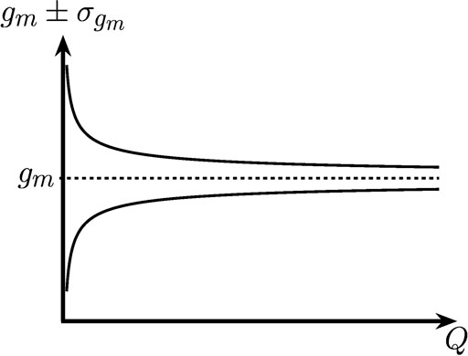
FIGURE 3. Sketch of the m’the component of Capon’s estimator and the corresponding $1\sigma$-error subject to the sample size Q. The error declines as $1/\sqrt{Q}$.

5 Summary and Outlook

The analysis of the error propagation is of major importance for the application of linear inversion methods. Within a linear approximation, upper bounds for the errors of Capon’s estimator resulting from measurement errors and measurement position errors are derived. These upper bounds solely depend on known quantities, i.e., measurements and measurement positions, whereas the true estimation error cannot be calculated within the practical application of the method, since the accurate estimator is unavailable. It turns out that Capon’s method provides the same error propagation as the least square fit method. These two methods differ in the filter matrices which weight or eliminate parts of the data in different ways. Since these matrices are applied to the same set of measurements, the different weighting of the data or the elimination of subsets does not reduce the errors. The condition number of the shape matrix is the key parameter for the error propagation, since it determines how the errors are amplified. The measurement errors as well as the measurement position errors have to be estimated from the measurements. For a given underlying model, the condition number of the shape matrix solely depends on the measurement positions. Thus, the amplification of the errors can be reduced by choosing preferred data points.

Furthermore, Capon’s method is based on the evaluation of statistically averaged data. For the practical application of the method only a finite number Q of samples is available. This limited number of samples results in an error of Capon’s estimator which can be derived by regarding Capon’s method as a special case of the maximum likelihood estimator. The more samples are available, the smaller the error becomes, since the error declines as $1/\sqrt{Q}$.

As a follow-up of the generalized derivation of Capon’s method, the present work establishes the mathematical basis of Capon’s error propagation for the practical application of the method.

Appendix: Matrix Power of the Data Covariance Matrix

For the calculation of Capon’s estimator the inverse data covariance matrix ${\underset{¯}{\underset{¯}{M}}}^{-1}$ is necessary. First of all it should be noted that the inverse exists due to the averaging process, whereas the matrix $\underset{¯}{B}\circ \underset{¯}{B}$ is not invertible [3]. In the case of a vanishing standard deviation (${\sigma }_n=0$), the application of the diagonal loading technique [3] guarantees the existence of the inverse data covariance matrix, since the condition number of $\underset{¯}{\underset{¯}{M}}$ is close to unity at the optimal diagonal loading parameter.

Furthermore, there exists a unitary transformation $\underset{¯}{\underset{¯}{V}}$ so that

$\underset{¯}{\underset{¯}{M}}=\underset{¯}{\underset{¯}{V}}{\underset{¯}{\underset{¯}{D}}}_{\underset{¯}{\underset{¯}{M}}}{\underset{¯}{\underset{¯}{V}}}^{-1}(93)$

where

${\underset{¯}{\underset{¯}{D}}}_{\underset{¯}{\underset{¯}{M}}}=\text{diag}\left[{\lambda }_1,\dots ,{\lambda }_n\right](94)$

is a diagonal matrix that contains the eigenvalues of $\underset{¯}{\underset{¯}{M}}$. Therefore, the inverse data covariance matrix results in

${\underset{¯}{\underset{¯}{M}}}^{-1}={\left[\underset{¯}{\underset{¯}{V}}{\underset{¯}{\underset{¯}{D}}}_{\underset{¯}{\underset{¯}{M}}}{\underset{¯}{\underset{¯}{V}}}^{-1}\right]}^{-1}=\underset{¯}{\underset{¯}{V}}{\underset{¯}{\underset{¯}{D}}}_{\underset{¯}{\underset{¯}{M}}}^{-1}{\underset{¯}{\underset{¯}{V}}}^{-1},(95)$

where

${\underset{¯}{\underset{¯}{D}}}_{\underset{¯}{\underset{¯}{M}}}^{-1}=\text{diag}\left[{\lambda }_1^{-1},\dots ,{\lambda }_n^{-1}\right].(96)$

Further transformation delivers

$\begin{array}{c}{\underset{¯}{\underset{¯}{M}}}^{-1}=\underset{¯}{\underset{¯}{V}}{\underset{¯}{\underset{¯}{D}}}_{\underset{¯}{\underset{¯}{M}}}^{-1}{\underset{¯}{\underset{¯}{V}}}^{-1}\\ =\underset{¯}{\underset{¯}{V}}{\underset{¯}{\underset{¯}{D}}}_{\underset{¯}{\underset{¯}{M}}}^{-1/2}{\underset{¯}{\underset{¯}{D}}}_{\underset{¯}{\underset{¯}{M}}}^{-1/2}{\underset{¯}{\underset{¯}{V}}}^{-1}\\ =\underset{¯}{\underset{¯}{V}}{\underset{¯}{\underset{¯}{D}}}_{\underset{¯}{\underset{¯}{M}}}^{-1/2}{\underset{¯}{\underset{¯}{V}}}^{-1}\underset{¯}{\underset{¯}{V}}{\underset{¯}{\underset{¯}{D}}}_{\underset{¯}{\underset{¯}{M}}}^{-1/2}{\underset{¯}{\underset{¯}{V}}}^{-1}\\ ={\underset{¯}{\underset{¯}{M}}}^{-1/2}{\underset{¯}{\underset{¯}{M}}}^{-1/2}\end{array}(97)$

so that the square root of the inverse data covariance matrix is defined as

${\underset{¯}{\underset{¯}{M}}}^{-1/2}=\underset{¯}{\underset{¯}{V}}{\underset{¯}{\underset{¯}{D}}}_{\underset{¯}{\underset{¯}{M}}}^{-1/2}{\underset{¯}{\underset{¯}{V}}}^{-1}(98)$

where

${\underset{¯}{\underset{¯}{D}}}_{\underset{¯}{\underset{¯}{M}}}^{-1/2}=\text{diag}\left[{\lambda }_1^{-1/2},\dots ,{\lambda }_n^{-1/2}\right].(99)$

Data Availability Statement

The original contributions presented in the study are included in the article/Supplementary Material, further inquiries can be directed to the corresponding author.

Author Contributions

All authors contributed conception and design of the study; ST and UM wrote the first draft of the manuscript; All authors contributed to manuscript revision, read and approved the submitted version.

Funding

We acknowledge support by the German Research Foundation and the Open Access Publication Funds of the Technische Universität Braunschweig. The work by YN is supported by the Austrian Space Applications Program at the Austrian Research Promotion Agency under contract 865967. DH was supported by the German Ministerium für Wirtschaft und Energie and the German Zentrum für Luft-und Raumfahrt under contract 50 QW1501.

Conflict of Interest

The authors declare that the research was conducted in the absence of any commercial or financial relationships that could be construed as a potential conflict of interest.

The reviewer LZ declared a past collaboration with one of the authors YN to the handling editor.

Acknowledgments

The authors are grateful for stimulating discussions and helpful suggestions by Karl-Heinz Glassmeier, Patrick Kolhey and Alexander Schwenke.

References

1. Capon J. High-resolution Frequency-Wavenumber Spectrum Analysis. Proc IEEE (1969) 57:1408–18. doi:10.1109/PROC.1969.7278

CrossRef Full Text | Google Scholar

2. Toepfer S, Narita Y, Heyner D, Motschmann U. The Capon Method for Mercury's Magnetic Field Analysis. Front Phys (2020) 8:249. doi:10.3389/fphy.2020.00249

CrossRef Full Text | Google Scholar

3. Toepfer S, Narita Y, Heyner D, Kolhey P, Motschmann U. Mathematical Foundation of Capon's Method for Planetary Magnetic Field Analysis. Geosci Instrum Method Data Syst (2020) 9:471–81. doi:10.5194/gi-9-471-2020

CrossRef Full Text | Google Scholar

4. Motschmann U, Woodward TI, Glassmeier KH, Southwood DJ, Pinçon JL. Wavelength and Direction Filtering by Magnetic Measurements at Satellite Arrays: Generalized Minimum Variance Analysis. J Geophys Res (1996) 101:4961–5. doi:10.1029/95JA03471

CrossRef Full Text | Google Scholar

5. Su W, Gu H, Ni J, Liu G. Performance Analysis of MVDR Algorithm in the Presence of Amplitude and Phase Errors. IEEE Trans Antennas Propagat (2001) 49(12):1875–7. doi:10.1109/8.982472

CrossRef Full Text | Google Scholar

6. Narita Y. A Note on Capon’s Minimum Variance Projection for Multi-Spacecraft Data Analysis. Front Phys (2019) 7:121. doi:10.3398/fphy.2019.00008

CrossRef Full Text | Google Scholar

7. Sahraoui F, Belmont G, Rezeau L, Cornilleau-Wehrlin N, Pinçon JL, Balogh A. Anisotropic Turbulent Spectra in the Terrestrial Magnetosheath as Seen by the Cluster Spacecraft. Phys Rev Lett (2006) 96:7. doi:10.1103/PhysRevLett.96.075002

CrossRef Full Text | Google Scholar

8. Huang SY, Zhou M, Sahraoui F, Deng XH, Pang Y, Yuan ZG, et al. Wave Properties in the Magnetic Reconnection Diffusion Region with Highβ: Application of Thek-Filtering Method to Cluster Multispacecraft Data. J Geophys Res (2010) 115:17–9. doi:10.1029/2010JA015335

CrossRef Full Text | Google Scholar

9. Narita Y, Comişel H, Motschmann U. Spatial Structure of Ion-Scale Plasma Turbulence. Front Phys (2014) 2:13. doi:10.3389/fphy.2014.00013

CrossRef Full Text | Google Scholar

10. Roberts OW, Li X, Jeska L. A Statistical Study of the Solar Wind Turbulence at Ion Kinetic Scales Using the K-Filtering Technique and Cluster Data. ApJ (2015) 802:1. doi:10.1088/0004-637X/802/1/2

CrossRef Full Text | Google Scholar

11. Wang T, Cao J, Fu H, Meng X, Dunlop M. Compressible Turbulence with Slow-Mode Waves Observed in the Bursty Bulk Flow of Plasma Sheet. Geophys Res Lett (2016) 43(5):1854–61. doi:10.1002/2016GL068147

CrossRef Full Text | Google Scholar

12. Zhang L, He J, Narita Y, Feng X. Reconstruction Test of Turbulence Power Spectra in 3D Wavenumber Space with at Most 9 Virtual Spacecraft Measurements. J Geophys Res Space Phys (2021) 126:e2019JA027413. doi:10.1029/2019JA027413

CrossRef Full Text | Google Scholar

13. Narita Y, Plaschke F, Magnes W, Fischer D, Schmid D. Error Estimate for Fluxgate Magnetometer In-Flight Calibration on a Spinning Spacecraft. Geosci Instrum Method Data Syst (2021) 10:13–24. doi:10.5194/gi-10-13-202

CrossRef Full Text | Google Scholar

14. Werner D. Funktionalanalysis. Berlin: Springer (2007)

15. Belsley DA, Kuh E, Welsch RE. The Condition Number, Regression Diagnostics: Identifying Influential Data and Sources of Collinearity. New York: Wiley (1980). p. 100–4.

16. Gauß CF. (1839) Allgemeine Theorie des Erdmagnetismus: Resultate aus den Beobachtungen des magnetischen Vereins im Jahre 1838, editorsCF Gauss, and W Weber. Leipzig: Weidmannsche Buchhandlung (1839). p. 1–57.

17. Glassmeier K-H, Tsurutani BT. Carl Friedrich Gauss—General Theory of Terrestrial Magnetism—A Revised Translation of the German Text. Hist Geo Space Sci (2014) 5:11–62. doi:10.5194/hgss-5-11-2014

CrossRef Full Text | Google Scholar

18. Toepfer S, Narita Y, Glassmeier K-H, Heyner D, Kolhey P, Motschmann U, et al. The Mie Representation for Mercury's Magnetic Field. Earth Planets Space (2021) 73:65. doi:10.1186/s40623-021-01386-4

CrossRef Full Text | Google Scholar

19. Dodelson S. Modern Cosmology. London: Academic Press (2003).