Abstract
Numerous worm and arthropod species form physically-connected aggregations in which interactions among individuals give rise to emergent macroscale dynamics and functionalities that enhance collective survival. In particular, some aquatic worms such as the California blackworm (Lumbriculus variegatus) entangle their bodies into dense blobs to shield themselves against external stressors and preserve moisture in dry conditions. Motivated by recent experiments revealing emergent locomotion in blackworm blobs, we investigate the collective worm dynamics by modeling each worm as a self-propelled Brownian polymer. Though our model is two-dimensional, compared to real three-dimensional worm blobs, we demonstrate how a simulated blob can collectively traverse temperature gradients via the coupling between the active motion and the environment. By performing a systematic parameter sweep over the strength of attractive forces between worms, and the magnitude of their directed self-propulsion, we obtain a rich phase diagram which reveals that effective collective locomotion emerges as a result of finely balancing a tradeoff between these two parameters. Our model brings the physics of active filaments into a new meso- and macroscale context and invites further theoretical investigation into the collective behavior of long, slender, semi-flexible organisms.
1 Introduction
Throughout the living world, interactions among individuals, and between individuals and the environment, give rise to emergent collective phenomena across scales: cell migration, flocking birds, schooling fish, and human crowds moving in unison [1–4]. While most examples of collective behavior occur in regimes without physical contact among individuals, many insect, arthropod, and worm species form dense aggregations, where constituent individuals are in constant physical contact with each other, for the purposes of survival, foraging, migration, and mating [5–7]. Small-scale interactions among individuals enable emergent functionalities at the group level, such as the formation of adaptive structures, including fire ant rafts [8], army ant bridges [9], and bee clusters [10], that can enhance the survival of the aggregation compared to solitary individuals. These living aggregations, where the constituents exert forces on each other or even entangle their bodies into a single mass [6, 11], are associated with the world of soft active matter, which comprises a wide range of systems in which self-propelled individuals can convert energy from the environment into directed motion [7, 12–14].
Here, we examine the aggregation and swarming behavior of active polymer-like organisms, such as worms, that are flexible and characterized by their slender bodies (i.e., each possessing a length much longer than the width). Some species of worms can physically braid their bodies into highly entangled aggregations [11, 15–17]. In this paper, we focus on Lumbriculus variegatus, an aquatic worm also known as the California blackworm or mudworm. Blackworms are approximately 1 mm in diameter and up to 2–4 cm in length and live in shallow, marshy conditions across the Northern Hemisphere [11]. The physiology, neurology, biology, and behavior of individual L. variegatus has been extensively studied [11, 18–20], while their collective behavior has only recently been examined [17]. Blackworms can form entangled, shape-shifting blobs which allow the constituent worms to protect themselves against environmental stressors and to preserve moisture in dry conditions [17]. Recent experiments have quantified the material properties and aggregation dynamics of blackworm blobs, which can contain anywhere from a few to over tens of thousands worms and behave as a non-Newtonian fluid [17].
Most notably, these experiments resulted in the first observation of emergent locomotion in an entangled aggregation of multicellular organisms and robophysical models. While some physically-connected aggregations of worms and arthropods have been observed to demonstrate collective, coordinated movement and migration (e.g., [21, 22]), the blackworm blobs demonstrated collective self-transport in temperature gradients [17]. Under high light intensity, the worms remained a single entangled unit as they moved toward cooler environments, but only about 70% of worms moved together as an entangled blob in the absence of the spotlight [17]. It was observed in small blobs that the mechanism of this collective movement lies in a differentiation of activity, with outstretched “puller” worms in the front pulling the coiled, raised “wiggler” worms at the back [17]. This phenomenon was also captured in robophysical models of “smarticle” robots, indicating the importance of this mechanism in the self-motility of an entangled collective [17].
Other recent work has investigated the rheology and phase separation in aggregations of a similar organism, T. tubifex, also called the sludge worm or sewage worm. These worms also form highly entangled blobs in water to minimize exposure to poisonous dissolved oxygen, though collective locomotion has not been observed [16, 23]. The authors of this work showed that the dynamics observed in their experiments could not be captured by modeling blobs as coalescing droplets undergoing Brownian motion [16]. Namely, the diffusion constant of the blobs, which describes how quickly the blobs explore space, was observed to be independent of their size, rather than scaling as the inverse of the blob radius as would have been expected assuming completely random motion; this discrepancy was attributed to the active random motion of worms at the surface of the blob. Moreover, it was asserted that a model of collective worm behavior would likely need to account for the self-propelled tangentially-driven motion of individual worms [23].
Motivated by these experiments and insights on aggregations of blackworms and sludge worms [16, 17, 23], we pursue a theoretical model that captures the collective behavior of aquatic worms by linking together local rules governing interactions between individual worms with the emergent macroscale dynamics of the blob. Worms consume energy in order to propel themselves; hence, we look toward the extensive body of research in modeling active polymers and worm-like filaments [24, 25], where activity can be implemented in different ways, such as by immersing the polymer in a bath of colored or non-Gaussian noise [26, 30–32], or via monomers driven by active forces [27–29, 33]. In general, application of these models has been geared toward biopolymers and unicellular organisms in the microscopic regime, such as actin filaments, microtubules, cilia and flagella, and swarms of slender bacteria [24, 28, 34–37]. In this paper, we adapt the physics of active filaments to a macroscale, whole-organism context in order to characterize the collective behavior of worm blobs.
A similarly polymer-like organism that has also demonstrated aggregation and swarming is the nematode C. elegans, which is about an order of magnitude smaller than the blackworm [38]. Agent-based modeling was used to elucidate the behavioral rules governing collective C. elegans behavior [38], in which individual nematodes were modeled in polymer-like fashion as nodes connected by springs, with the head node undergoing a persistent random walk and the rest of the body following.
Here, we are primarily interested in tangentially-driven active filaments [27, 28], as their behavior is qualitatively similar to that of worms. Such semi-flexible, tangentially-driven filaments demonstrate a rich diversity of behavior. The bending rigidity, activity, aspect ratio, and density of filaments define phases of flocking, spiraling, clustering, jamming, and nematic laning [28].
Drawing upon these models, we model worms as two-dimensional active Brownian polymers, driven by experimental observations of the behavior of single worms (Figure 1A), worm blobs (Figure 1B), and the collective locomotion of worm blobs in temperature gradients (Figure 1C; [17]). We model each worm as a polymer with a tangential self-propulsion force acting only on a portion of the worm designated as the head end, as this qualitatively reflects our observations of worms being more active at the head (Figure 1D). After developing this single-worm model, we simulate worm blobs via aggregation of multiple identical worms (Figure 1E) attracted to each other via an interaction potential.
FIGURE 1
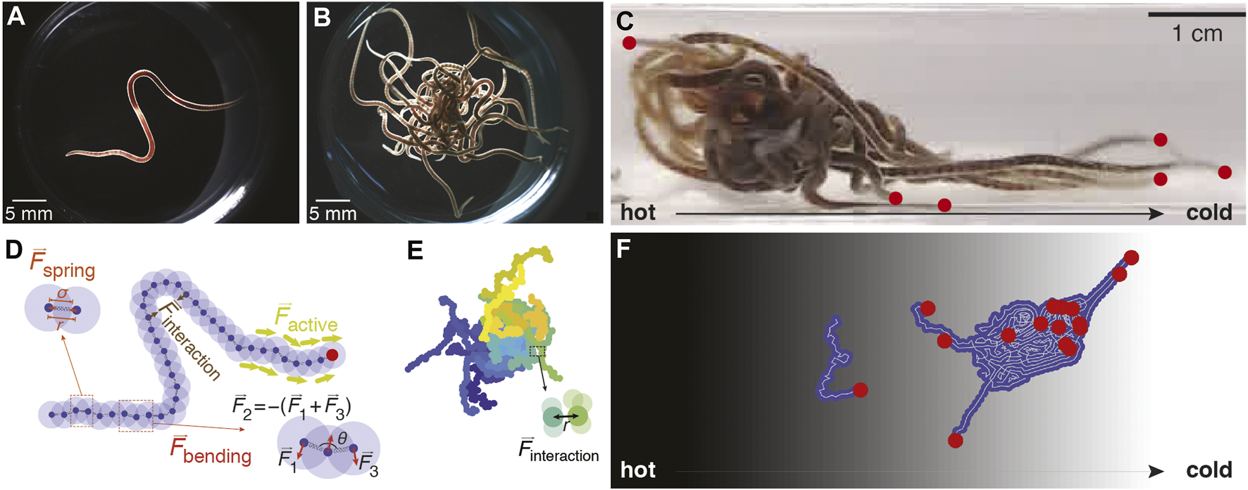
Worm-inspired active polymer model. (A). A single California blackworm (L. variegatus). (B). An entangled worm blob consisting of 20 worms. (C) An entangled worm blob ( ∼20 worms) in a temperature gradient displays collective locomotion toward the cold side (right), with “puller” worms extending from the front (worm heads marked by red dots). (D). Polymer model of single worm consisting of 40 monomers connected by springs with interaction potential described in Eq. 1. The “head” section (with the distal head node indicated by the red dot) of the worm is subject to a constant-magnitude tangential force generating self-propulsion. The spring force (Eq. 2) is computed for adjacent pairs of monomers, and the bending force (Eq. 3) for adjacent triplets of monomers. The interaction force (Eq. 1) is computed for every pair of monomers in a chain and is attractive if the monomers are further apart than the equilibrium distance σ and repulsive if they are closer than σ. (E). Simulated worm blob consisting of 20 polymers. Each color represents a different worm. The interaction force (Eq. 6) is computed for every pair of monomers and is stronger between monomers of different chains. (F). Simulated worm blob in a temperature gradient with the hotter side on the left (black background) and the colder side on the right (white background) demonstrates collective locomotion toward the cold side. Red dots indicate the head ends of each worm; some worm heads protrude from the bulk of the blob.
We then simulate worm blobs in a temperature gradient, which sets a preferred direction of the worm toward the cold side, reflecting real worms’ preference for cooler temperatures in analogous experimental setups [17]. We perform a parameter sweep over the strength of attraction between worms and the magnitude of the tangential force. We find that from the resulting rich phase diagram, collective locomotion arises only when the attraction strength and tangential force are finely balanced (Figure 1F). Though our model is in 2-D, it captures the emergent collective locomotion of the worm blob as observed in experiments [17].
2 Active Polymer Model
To construct our model, we begin by modeling a single worm as a polymer: a series of individual monomers linked together by springs of equal length (Figure 1D). The monomers are subject to three potentials: interaction (Uinteraction), spring (Uspring), and bending (Ubending) [39, 40]:where Nm is the number of monomers per chain, rij = rj −ri is the vector between the positions of monomers i and j, σ is the equilibrium length of the spring connecting two adjacent monomers, ks is the spring constant, and kb is the bending stiffness. The bending potential Ubending, described by a harmonic angle potential, is computed for every consecutive triplet of monomers i, i + 1, i + 2 whose connecting springs form an angle ϕi,i+1,i+2 = cos−1(ri+1,i ⋅ri+1,i+2/|ri+1,i||ri+1,i+2|). ϕ0 is the equilibrium angle of each adjacent pair of springs and is set to π.
The interaction potential is inspired by the Lennard-Jones potential used to describe interatomic interactions [39]. We use a modified form of this potential as it captures strong short-range repulsion and weaker long-range attraction, though with slightly smaller exponents that enable computational efficiency with qualitatively similar results. For two monomers with a separation r < σ, the interaction potential mimics an excluded volume mechanism to prevent the monomers from occupying the same space. For two monomers with separation r > σ, the potential is weakly attractive. This results in the polymer forming a more coiled-up conformation. The coiling up is offset partially by the bending potential, which acts to straighten the polymer.
At each step of the simulation, the force on each monomer is computed:and the position of each monomer is updated via the overdamped equation of motionwhere is a two-dimensional random vector with each component sampled from the normal distribution with mean 0 and variance 1, such that represents noise with standard deviation given by a temperature value T.
L. variegatus cultivated in the laboratory measured approximately 25 ± 10 mm in length with a radius of 0.6 ± 0.1 mm, corresponding to an average length-to-radius ratio of approximately 40. In our model, each pair of monomers is connected by a spring with equilibrium length σ, which is also set to be the equilibrium distance at which the interaction potential of each monomer has value 0. In our simulations, we model worms that are N = 40 monomers long, such that each worm can be considered to have a length of 41 σ with radius σ, corresponding to a length-to-radius ratio of 41. We also set the spring coefficient ks = 5,000, a relatively high value as worms do not easily stretch along their axis. We also set the bending coefficient kb = 10, an intermediate value that results in more elongated worms at low temperatures and coiled worms at high temperatures (2A-D). This bending coefficient is also partially offset by a interaction of ɛ = 1. The model parameters are tabulated in Table 1.
TABLE 1
| Parameter | Description | Range of values |
|---|---|---|
| N m | Number of monomers | 40 |
| Σ | Equilibrium distance between monomers | 1.189 (arb. units) |
| ɛ | Interaction coefficient, single worm | 1 |
| k s | Spring constant | 5000 |
| k b | Bending stiffness | 10 |
| F active | Self-propulsion force magnitude | 220–440 |
| ɛ blob | Interaction coefficient for blob (attraction parameter) | 2–22 |
List of model parameters and corresponding ranges of values used in simulations.
The dynamics of the simulated worm-like polymer are governed by the imposed thermal fluctuations, and as such the polymer is expected to exhibit Brownian motion. However, previous studies have indicated that a Brownian depiction does not accurately describe worm behavior [16]. We also observe that simulated worms in this Brownian model demonstrate little exploration of the simulation arena (e.g., low mean squared displacement) at low temperatures, with greater exploration at high temperatures due to large random fluctuations. However, in our observations of real L. variegatus, blackworms often demonstrate greater exploration at low temperatures (Figure 2A). Thus, we add an additional active force that reflects the self-propelled forward peristaltic crawling of the worm (Figure 1). The force acts with equal magnitude on eight monomers at one end of the worm, denoted the head end, in the tangential direction determined by averaging the position vectors of the links on either side of the monomer; that is, . This also reflects our observation that the worms in experiments demonstrate more activity at their heads than from the rest of their bodies.
FIGURE 2
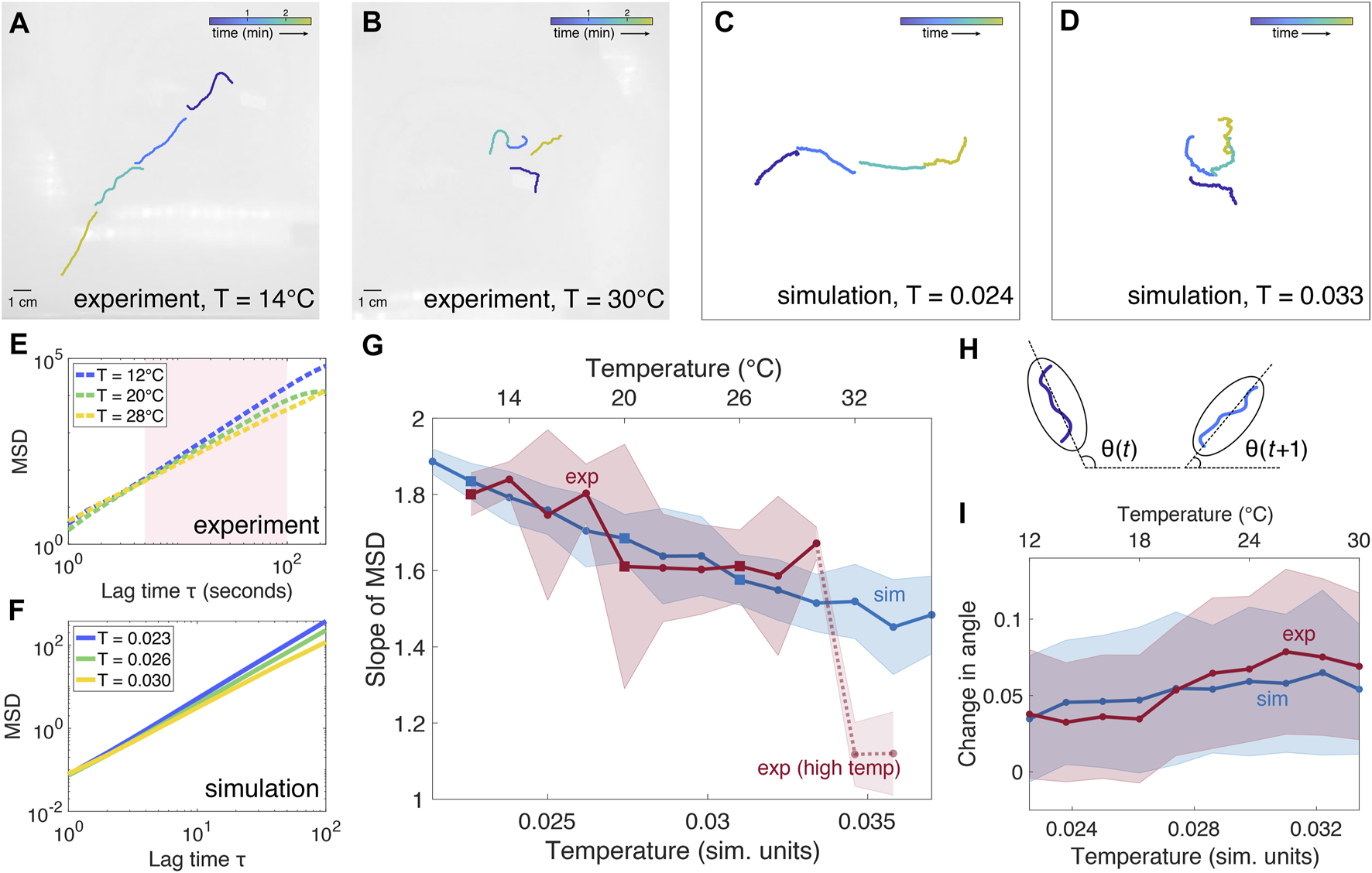
Active polymer model of a single worm. (A–B): Snapshots of single worm experiments at T = 14°C and T = 30°C, respectively. Worms are colored in software to visualize time progression. (C–D): Snapshots of simulated single worm conformations at T = 0.024 and T = 0.033 (simulation units), respectively. (E): Examples of mean squared displacement (MSD) as a function of lag time τ from three separate experimental trials at three different temperatures, indicated by the squares in panel (G). Because the MSD is not linear over the entire range of τ, the slope is computed for the region shaded in pink. (F): Examples of MSD from three simulations at three different temperatures, indicated by the squares in panel (G). (G): Comparison of mean slope ± SD of mean squared displacement (MSD) as a function of temperature for simulation (blue) and experiment (red, 5 trials). The slope of MSD generally decreases with increasing temperature. Experimental data at T = 32–34°C are indicated by a dashed line, as worm physiology is likely to be affected by the high temperature. Squares indicate temperatures at which examples of MSD are plotted in panels (E–F). (H): The angle θ at time t is computed by fitting an ellipse to the worm and calculating the angle of the major axis with respect to the horizontal. The average change in angle between consecutive timesteps θ(t + 1) −θ(t) is used as a measure of worm fluctuations. (I): For the trials analyzed in panel (G), the average change in angle θ increases with temperature for both simulation and experiment.
To fit the parameters of the model (Table 1) to reflect the observed behavior of blackworms, we compare simulations with single-worm experiments (Figures 2A,B). Blackworms obtained from Aquatic Foods and Blackworm Co. (CA, United States) and were cultivated in several boxes (35 cm × 20 cm × 12 cm, 25 g of worms per box) filled with spring water (at a height of approximately 2 cm) at ∼4°C for at least 3 weeks. Worms were habituated to room temperature in a 50 ml beaker with spring water at ∼20°C at least 6 h prior to experiments. Worms were fed with tropical fish flakes twice a week, and the water was changed 1 day after feeding them. Studies with L. variegatus do not require approval by the institutional animal care committee.
In these experiments, a single worm was placed in the center of a 30 cm × 30 cm × 1 cm container filled with water at a height of approximately 0.5 cm. We recorded experiments at water temperatures from 12 to 34°C ± 1°C in increments of 2°C. The worm behavior was recorded at a rate of two frames per second for 15 min. Video frames were analyzed using MATLAB Image Processing Toolbox (MathWorks, Natick, MA, United States) to extract the position and geometry of the worm. Example trajectories of the tracked worms are animated in Supplementary Video S1–S4 and plotted in Supplementary Figures S1–S12.
We observe that at temperatures of 30°C or lower, the worm tends to explore the arena. Often, the worm will travel in a relatively straight path until it reaches the wall of the container, after which it will then continue to explore along the edge of the wall. In some cases, the worm fails to find the wall and continues to explore somewhat erratically. Beyond 30°C, the worm exhibits significantly less exploration, staying close to its original starting position. We attribute this to the temperature being too high for the worm to comfortably explore, and potentially even causing physiological changes to the worm [41]. Above 34°C, the worm is unlikely to survive for more than a few minutes if not seconds.
In our simulations, the self-propelled Brownian polymer remains subject to Gaussian thermal fluctuations. Most noticeably at low T, the active tangential force results in the simulated worm moving persistently in a single direction (Figure 2C). At high T, the thermal fluctuations tend to dominate over the bending potential, resulting in a coiled-up conformation of the simulated worm, and as such the individual tangential forces are likely to effectively cancel each other out in direction, resulting in lower overall displacement (Figure 2D, also see Supplementary Video S5–S7).
To compare simulation and experiment, we examine the mean squared displacement (MSD) as a function of lag time τ (Figures 2E–G; Supplementary Figures S1–S12). Our key observation is that the slope of the MSD, when plotted on a logarithmic scale, differs depending on the temperature. A higher MSD slope indicates that the worm undergoes more directed motion, while a lower MSD slope indicates more diffusive motion, with a slope of one representing Brownian motion. In both experiment and simulation, the slope of the MSD generally decreases as temperature increases: at low temperatures, the worm displays near-ballistic movement, which becomes increasingly less directed as temperature increases. Because the worm is confined in the experiments, the MSD is limited by the size of the arena and begins to plateau at large values of τ. Hence, we calculate the slope for the regime in which the logarithm of MSD is generally linear, for τ between 5 and 100. The simulated worm is not subject to boundary conditions and, at low T, will move persistently in the direction set by its initial orientation.
By comparing the slope of the MSD from experiments with simulations, we derive a rough scaling of the temperature between simulation units (Tsim) and degrees Celsius (Texp): Texp = (5,000/3)Tsim − 77/3. In determining this scaling, we excluded experimental data above 30°C, due to the drastic decrease in worm activity at high temperatures. Hence, this scaling is valid only for temperatures between 12 and 30°C inclusive.
While the slope of the MSD captures whether the worm’s motion is directed or random, it does not capture higher-order measures of worm activity. To examine the amount by which a worm fluctuates over time, we calculate the average change in angle of the worm between consecutive timesteps (Figures 2H,I). The angle θ is determined by fitting the smallest ellipse that encloses the worm and calculating the angle of the major axis with respect to the horizontal direction (Figure 2H). The change in angle increases with temperature, reflecting the greater fluctuations observed in both simulation and experiment.
3 Worm Blob Aggregation
To model a collective system of worms, we retain the dynamics of the single-worm model, but specify a stronger interaction potential between monomers of different chains:where M is the number of worms in the system, Nm is the number of monomers per worm, is the vector between the positions of monomer i of chain g and monomer j of chain h, and the coefficient ɛblob > ɛ. We refer to ɛblob as the attraction parameter governing the strength of attractive forces between worms.
We observe in experiments that temperature affects the attachment of worms in a blob, resulting in a transition between a solid-like phase to a fluid-like phase (Figure 3A). At a low temperature (10°C), a tightly entangled blob remains approximately the same size over the course of several minutes. At a moderate temperature (25°C), the worms spread out slightly, though the blob remains intact; at a high temperature (35°C), the worms quickly disentangle from one another, forming a fluid of detached, coiled worms.
FIGURE 3
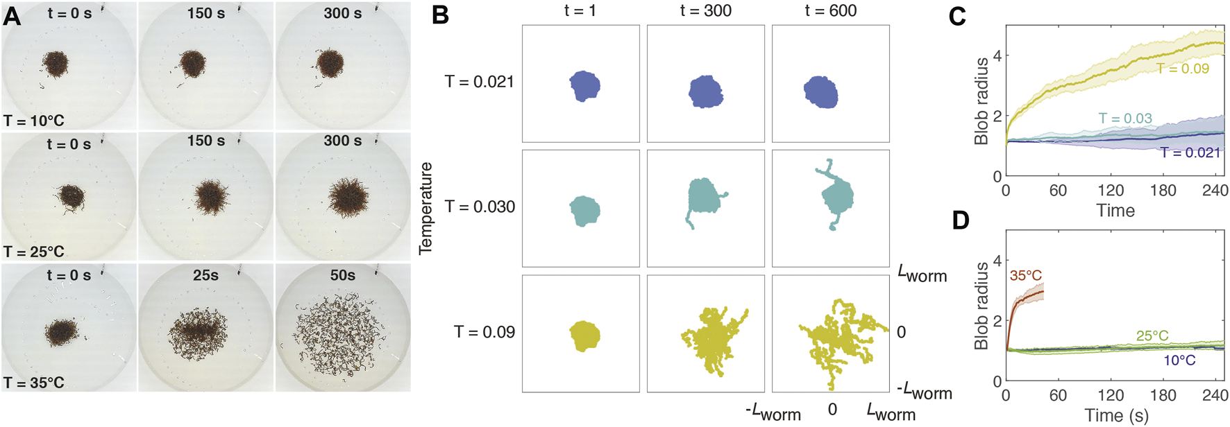
Temperature affects cohesion of worm blobs. (A): Snapshots of experimental blobs (N ∼ 600) at 10, 25, and 35°C. Experiments at T = 35°C were performed for only 1 min since worms begin to die after about 2 min at this temperature. The diameter of the dish is 20 cm. (B). Snapshots of simulated blobs at different temperatures (row) and time steps (column). Each box is a square with side twice the equilibrium length of one worm (Lworm = 41σ). Each blob contains 20 worms with attachment strength ɛblob = 12. (C): Mean radius ± SD of simulated blob as a function of time for different temperatures (T = 0.021 (dark blue), 0.03 (cyan), and 0.09 (yellow)), corresponding roughly to the experimental temperatures used in panel (A). For each trial, the radius is normalized to the initial radius at t = 0. (D): Mean radius ± SD of experimental blob (N ∼ 600) as a function of time for different temperatures (T = 10 (blue), 25 (green), 35 (red) °C). For each trial, the radius is normalized to the initial radius at t = 0.
We simulate worm blobs at three different temperatures, T = 0.021, 0.030, and 0.09 (Figure 3; Supplementary Video S8–S10). The first two temperatures roughly correspond to 10 and 25°C, respectively, following the temperature scaling described in Section 2. Since temperatures above 30°C result in drastic changes to worm behavior and scale differently than at moderate temperatures, we choose a high simulation temperature of 0.09 to represent 35°C. In these simulations, ɛblob was set to 12, and the active force magnitude was 220.
Each simulation (row of Figure 3B) begins from the same initial conditions shown in the t = 1 column. To generate these conditions, we perform a preliminary simulation starting from 20 worms initialized to random positions: the location of the head node was randomly sampled from a square with side length equal to half the worm length, with the angle of the worm sampled from the interval [0, 2π). This ensured that the worms were close enough to aggregate into a single blob. The worms were then allowed to aggregate at a low temperature, T = 0.02, for a period of 20 time steps. The interaction coefficient ɛblob was set to a high value of 20, and the active tangential force was set to zero (i.e., the worms obeyed Brownian dynamics) to facilitate attachment. The values of the parameters in this preliminary simulation are chosen such that this “equilibration” process results in worms attaching into a stable, densely-packed blob from random conditions. This same resulting blob was used as the starting point for all simulations described below.
At T = 0.021, the worms remain in a compact, solid-like blob, demonstrating little activity. At T = 0.030, a few worms begin to detach, but most of the worms remain tightly attached. However, at T = 0.090, the blob “melts” into a fluid-like state, as the worms separate from each other and disperse across the arena, corroborating the experimental results (Figure 3A).
4 Emergent Locomotion and Collective Thermotaxis
Previous experiments demonstrated the ability of biological worm blobs to undergo emergent collective locomotion in temperature gradients [17]. The blobs exhibited negative thermotaxis, moving from the high temperature side of the gradient to the low temperature side (Figure 4A). The collective locomotion was enhanced by shining a spotlight on the worms [17]: a worm blob subject to bright light conditions (5,500 lux) moved together as an entangled unit, resulting in over 90% of worms reaching the cold side over the course of the 30-min experiment. In contrast, worms under low room light conditions (400 lux) did not move as a compact blob, with most disentangling and moving individually, resulting in approximately 70% of worms successfully reaching the cold side in the same timeframe.
FIGURE 4
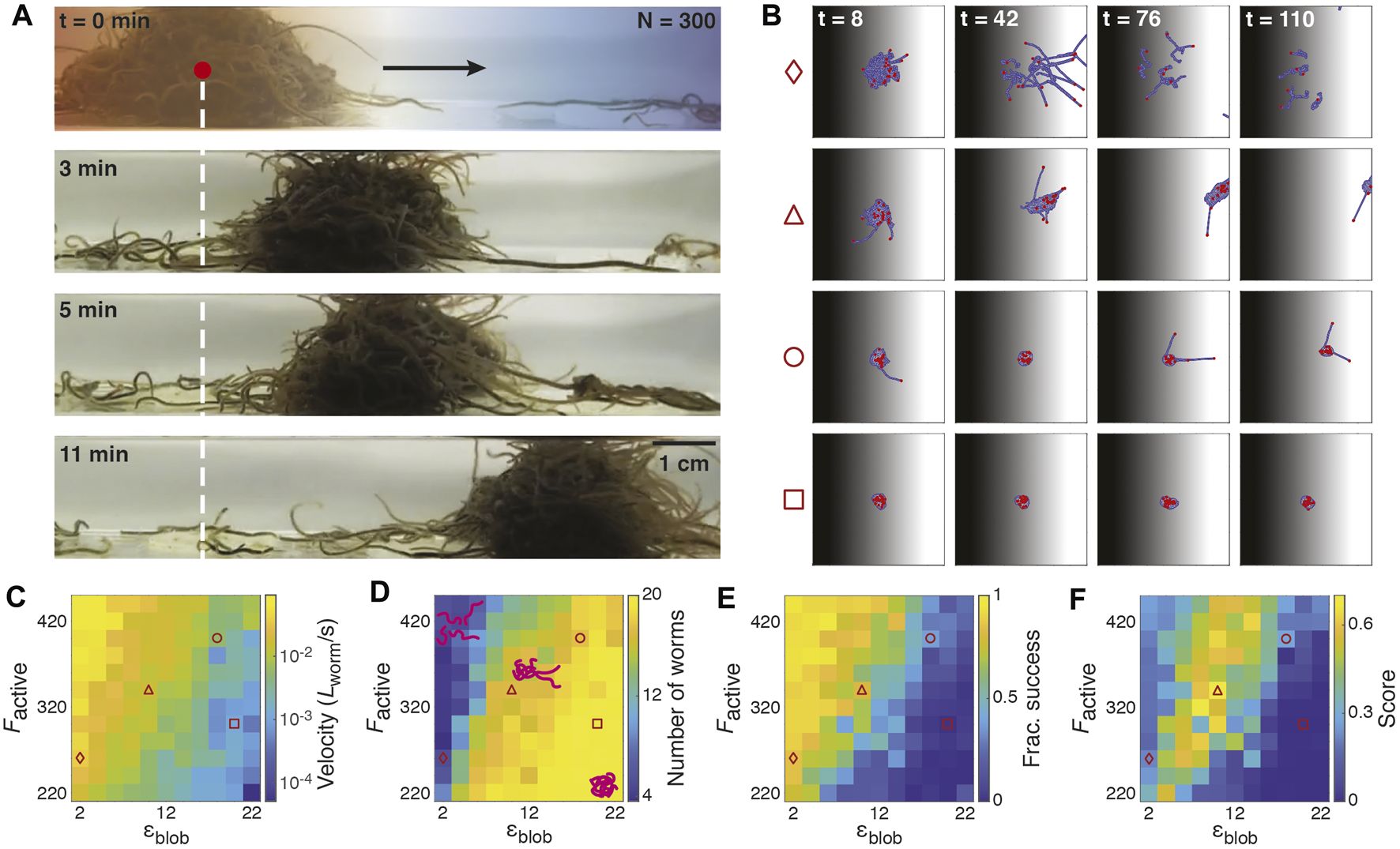
Emergent locomotion in temperature gradients. (A): Snapshots of an experimental worm blob (N = 300 worms) demonstrating emergent locomotion in a temperature gradient (left: high temperature; right: low temperature). (B): Snapshots of blob in temperature gradient from T = 0.08 (black) on the left to T = 0 (white) on the right. Each column corresponds to a different simulation time step (t = 8, 42, 76, and 110 respectively). Each row corresponds to different set of attraction parameters ɛblob and active force magnitudes Factive (diamond: ɛblob = 2, Factive = 260; triangle: ɛblob = 10, Factive = 340; circle: ɛblob = 18, Factive = 400; square: ɛblob = 20, Factive = 300). Red dots indicate the heads of individual worms. Despite the three-dimensional nature of real worm blobs, our two-dimensional model captures emergent collective locomotion for some combinations of ɛblob and Factive: in the triangle sequence, the majority of worms collectively move from the hot side of the gradient to the cold side, with the heads of some worms extending into the cold side. (C): Heatmap of the average x-component of the blob velocity (in worm length per second) for a range of Factive and ɛblob. The velocity is computed for the center of mass of the largest cohesive blob in the simulation. (D): Heatmap of the average number of worms (maximum of 20) of the largest cohesive blob for a range of Factive and ɛblob. Cartoons indicate typical configurations of worms for different regimes of parameter space. (E): Heatmap of the fraction of successful worms per simulation. Success is indicated by the fraction of worms that reach the T = 0 cold side of the gradient by the end of a 120-timestep simulation. (F): Heatmap of the collective locomotion score, given by the product of the blob velocity, blob size, and fraction of success, with each term weighted so that its maximum is 1 (Eq. 7).
In the single worm case, a simulated worm has no preferred direction in the absence of a gradient; if the temperature is low enough, the worm will move in the tangential direction dictated by its head end, but this direction relies only on the initial orientation of the worm, which is randomly chosen. A temperature gradient will break this symmetry and sets a preferred direction of motion. At high temperatures, the worm’s motion is largely random. However, if, via fluctuations, the head of the worm becomes oriented along the temperature gradient, pointing toward colder temperatures, the tangential forces will cause the worm to move in that direction. The further the worm moves toward lower temperatures, the more it will straighten out, resulting more pronounced ballistic motion. Inversely, if the worm is oriented such that it points toward warmer temperatures, the worm will continue to move in that direction if the surrounding temperature is low enough that the active force is not immediately dominated by random fluctuations. However, the component of the worm’s velocity parallel to the gradient will decrease as it moves toward higher temperatures, at which point fluctuations will dominate, and the worm more frequently reorients itself (Figure 2I).
Here, we simulate blobs in temperature gradients and observe that the level of attachment of worms in a blob depends on a tradeoff between the interaction coefficient ɛblob and active force magnitude Factive. The higher the interaction coefficient ɛblob, the more compact the blob, with worms tightly adhering to one another. Increasing the active force magnitude Factive, on the other hand, increases the likelihood that worms will break apart from the blob.
Simulated blobs with 20 worms were placed in a temperature gradient linearly decreasing from T = 0.08 on the left edge of the visualization area to T = 0 on the other edge. The visualization area corresponds to a square arena with each edge chosen to be 120 arbitrary units long, approximately 2.5 times the equilibrium length of a single worm. While only this region is visualized, the arena extends indefinitely in each direction, with a constant T = 0.08 beyond the left edge and T = 0 beyond the right edge.
Each temperature gradient simulation was run from the same initial conditions as described previously in Section 3, where the initial blob aggregated in the absence of a temperature gradient. The same initial blob was used for each simulation and was subsequently placed in the temperature gradient such that its center of mass was located in the center of visualization area, corresponding to T = 0.04. We then performed a systematic parameter sweep over the interaction coefficient ɛblob between values of 2–22 and the active force magnitude Factive between 220 and 420.
In Figure 4B, we highlight four examples of simulations from different regions of the explored parameter space that illustrate cases in which the blob successfully or unsuccessfully traverses the gradient as a collective. Simulations from a larger sampling of parameter space are also shown in Supplementary Video S11. If ɛblob is too low (diamond sequence), the worms do not remain attached; if ɛblob is too high (square sequence), the strong attachment forces dominate over the active forces, and the blob remains at its starting position. If ɛblob and Factive are balanced, this can lead to emergent cohesive locomotion toward the cold side of the gradient (triangle sequence). If ɛblob is slightly larger than Factive, collective locomotion may also occur, but at a slower speed (circle sequence).
In Figures 4C–E, we compare three quantities as a function of ɛblob and Factive: the velocity of the center of mass of the largest worm blob in the simulation, the size of the largest blob, and the fraction of worms that successfully reach the cold side of the gradient. Generally, we observe that each of these quantities is positively correlated with Factive and negatively correlated with ɛblob, or vice versa.
Figure 4C is a heatmap of the blob velocity as a function of Factive and ɛblob; as all of the worms in a given simulation may not be attached as a single aggregation, especially for lower values of ɛblob, we report here the velocity of the center of mass of the largest cohesive blob as identified using the DBSCAN clustering algorithm [42]. We use this algorithm to identify blobs of arbitrary size and shape where the separation between two monomers in a blob is no greater than 2σ, though many other clustering methods exist, with a range of applications across fields [43, 44]. We find here that the velocity increases as Factive increases, but decreases as ɛblob increases.
Meanwhile, Figure 4D shows a heatmap of the average number of worms in the largest blob, which shows the opposite trend as Figure 4C: the size of the blob is positively correlated with ɛblob but negatively correlated with Factive. For high ɛblob and low Factive, the blob remains completely cohesive, encompassing all 20 worms. For low ɛblob and high Factive, the worms are less cohesive, with the largest blobs containing down to about four worms.
Figure 4E illustrates the fraction of worms successfully reaching the cold side of the gradient per simulation. This heatmap parallels that of Figure 4C, showing that the highest proportion of success occurs for low ɛblob and high Factive, and the least successful blobs for high ɛblob and low Factive.
In general, simulated worms are most effective at reaching the cold side when ɛblob is low and Factive is high. However, they do not move cohesively, with the largest blobs containing between approximately 25–50% of the total worms in the simulation. At the other extreme, when ɛblob is high and Factive is low, nearly all worms remain in a cohesive aggregation, but the blob demonstrates little to no movement toward the cold side of the gradient, due to the attachment forces dominating over the active motion. We note that for real worms, remaining in a cohesive aggregation is beneficial, especially when there is danger of moisture loss [17]. Moreover, individual blackworms can die within minutes in high temperature environments (above 30°C). Our simulations do not reflect any potential worm death; in some cases, individual simulated worms that have moved toward the hot side of the gradient become “unstuck” via random fluctuations and may eventually find the cold side.
Hence, we seek a regime in which the worms demonstrate a high rate of success at reaching the cold side of the gradient and move relatively quickly while remaining mostly cohesive. To do so, we compute a score for each simulation given by the product of the velocity of the center of mass, largest blob size, and fraction of success, which each of the three terms normalized such that each individual term scales between 0 and 1. All three terms are moreover equally weighted such that the score takes on values between 0 and 1:where min(vblob, vmax) represents the smaller value between the average speed of the blob in the direction of decreasing temperature vblob, and v0, which is defined as half the width of the arena divided by the total simulation time (e.g., the slowest possible speed of a successful blob); and Nlargest blob is the number of worms in the largest blob.
Figure 4F illustrates this score as a function of ɛblob and Factive. The tradeoff between ɛblob and Factive produces a regime in which the highest scores are achieved, along a band that roughly follows the line Factive = 22ɛblob + 132.
Figure 5 illustrates a phase diagram corresponding to this function overlaid with example snapshots of blob configurations from corresponding simulations, revealing the rich ensemble of behaviors across the parameter space of Factive and ɛblob. To generate the phase diagram, we fit the score landscape from Figure 4F to the following function of Factive and ɛblob:
FIGURE 5
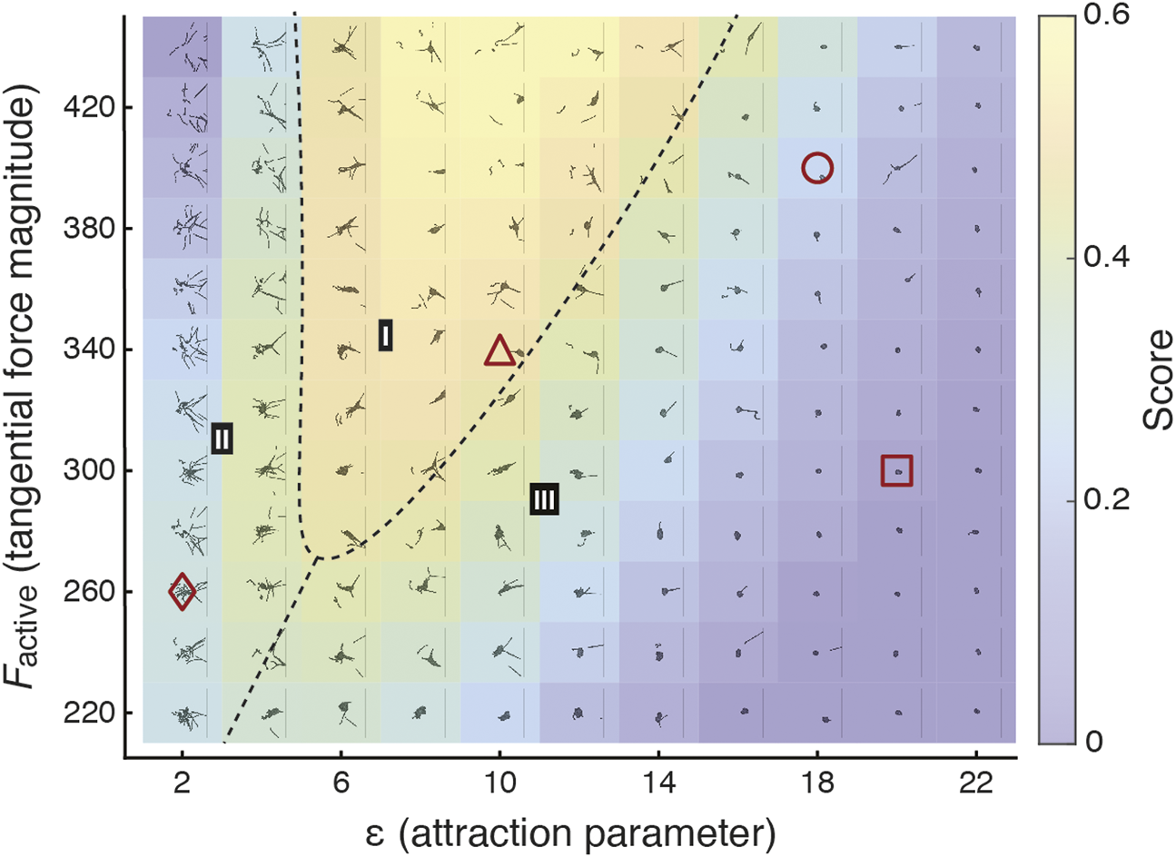
Heatmap of score reveals parameter regime in which the most effective collective locomotion is observed. The score illustrated in Figure 4F is fit to the function given in Eq. 8. The heatmap illustrates this fitted score function and is divided into three regimes (I-III). I: consistently successful cohesive blob locomotion, reflecting observed emergent locomotion in real worm blobs (Figure 4A); II: generally unsuccessful blob locomotion, with failure due to dissociation of blobs; III: generally unsuccessful blob locomotion, with failure due to overly strong attachment, resulting in little collective movement. In phases II and III, parameter combinations near the boundary of phase I can intermittently lead to successful collective locomotion. Each subpanel shows an overlaid snapshot at between t = 50 and 150 of an example simulation with the corresponding Factive and ɛblob. Red shapes correspond to example sequences shown in Figure 4B.
The parameters are tabulated in Supplementary Table S1.
The dashed lines in Figure 5 separate three regions (I-III) characterized by the prevailing collective behavior. In region I, corresponding to the region where the highest scores are achieved, the worms consistently traverse the gradient as a collective. In this region, the emergent collective locomotion reflects what is observed in experiments (Figures 1C, 4A; [17]). We note that while these real worm blobs inhabit three-dimensional space, our two-dimensional model nevertheless captures collective locomotion. In regions II and III, collective locomotion is generally unsuccessful, though successful cases of collective locomotion are intermittently observed near the boundary with region I. In region II, failures typically occur when the blob dissociates and worms move individually, as Factive is too high for the corresponding values of ɛblob. For failed cases in region III far from the boundary with region I, the worms are too strongly attached and as such the blob does not demonstrate any self-motility and remains near the starting position. Closer to the boundary with region I, the majority of worms may remain attached, with a few worms detaching from the blob and potentially moving toward the cold side on their own. The center of mass of the largest blob either remains close to the origin or drifts slowly to cold side, as here ɛblob is slightly too high compared to Factive.
5 Discussion
Following the first observation of collective locomotion in entangled worm blobs [17], we developed a model that employs the physics of active, semi-flexible polymers and filaments in the context of the collective behavior of macroscale, multicellular organisms. We model worms as self-propelled Brownian polymers, focusing specifically on the parameter space of aspect ratio, bending rigidity, activity, and temperature that describes the California blackworm, L. variegatus, at temperatures between 10 and 35°C. In the simulated single worm case, the constant-magnitude tangential force Factive results in a persistent directed motion at low temperatures, with larger fluctuations erasing the persistent motion at high temperatures. In a temperature gradient, this results in a preferred direction of movement from high to low temperatures.
Multiple simulated worms can aggregate into a blob, held together by attractive forces as governed by the attachment strength ɛblob. We show that the simulated blob can collectively navigate along a temperature gradient provided that the tangential force and attachment strength are balanced. In a parameter sweep over the attachment strength ɛblob and the magnitude of the tangential force Factive, we observe a tradeoff between the worm velocity and the cohesiveness of the blob. Higher attachment reduces the speed of the blob and hinders collective motion in extreme cases, while a higher force increases the individual worm speed but can result in worms detaching from the blob. We identify the regime where blob movement is “optimal” from a biological perspective–i.e., where the blob quickly moves toward cooler, less dangerous temperatures, while remaining largely cohesive, as worms are less likely to survive on their own outside of the blob–quantified by a score that combines the blob velocity, blob size, and fraction of worms successfully reaching the cold side of the gradient.
We note that a similar tradeoff, between the fraction of successful worms and the blob speed, was observed in experiments, as illustrated in Supplementary Figure S12 of [17]. For experiments at four different worm blob sizes (N = 10, 20, 40, and 80), it was observed that as the number of worms in a blob increased, the fraction of worms successfully reaching the cold side of the gradient increased as well. However, larger blobs were slower at reaching the cold side. While we have focused on a single blob size in this paper, our model can be expanded to other system sizes and can be used to make experimentally testable predictions of how the number of worms affects collective locomotion. Moreover, future experiments can involve altering the activity of individual worms (e.g. by adding alcohol to the water) and/or their attachment strength (e.g., by manipulating light conditions as observed in [17]) in order to test our predictions on these parameters’ effect on blob motility.
Currently, the parameters of our model are chosen such that there is qualitative agreement between the behavior of the simulated worm and observed L. variegatus. However, we expect that our model should be broadly generalizable to describe other long, slender, flexible organisms including annelids and nematodes. Future work will investigate the effect of the aspect ratio of individual worms on their collective behavior in temperature gradients. For instance, T. tubifex are a similar length to blackworms but are about a quarter as thick, though collective locomotion in T. tubifex has not been observed. Blob formation was also observed in terrestrial worms such as common earthworms (Lumbricus terrestris) and red wigglers (Eisenia fetida) [17], but collective locomotion in such worms remains to be investigated. Moreover, in the limit of an aspect ratio of 1, the polymer picture reduces to that of a single round particle. Such a model can be useful to describe aggregations of organisms that more closely resemble particles rather than filaments, such as ants and bees; future research can work toward a unified model that captures collective behavior along the gradient between active particles and filaments.
A primary limitation of our current model is its two-dimensionality. While we are able to capture collective behavior of active worm-like polymers, in reality, blackworms form blobs that are three-dimensional in nature. In sufficiently deep water, small blackworm blobs are hemispherical (Figure 4A). Future work will generalize the current model to three dimensions, which will also allow us to explicitly model the physical entanglement of polymers. Entanglement and reptation in polymer melts and solutions has been extensively examined for decades (e.g., by de Gennes [45]). More recently, non-equilibrium polymeric fluids containing active polymers have come under focus, as these systems cannot be explained by statistical-mechanical theories [24, 35, 46]. For instance, Manna and Kumar showed that in a confined volume, contractile active polymers spontaneously entangled, and moreover that this entangled state was stable for any volume fraction of polymers [46]. Meanwhile, for extensile active polymers, they observed a phase transition between disentanglement and entanglement governed by the activity and volume fraction.
In our current model, for simplicity, we have implemented self-propulsion of worms as a tangential force with constant magnitude, without consideration of the medium through which the worms are moving. In reality, worms harness friction to propel themselves, employing a combination of peristaltic elongation and contraction, undulatory strokes, and helical movements to crawl on surfaces, burrow through sediments, or swim through water [18, 47]. While our goal in this paper is to develop a parsimonious and generalizable description of worm behavior, accounting for hydrodynamics and friction can provide a more complete analysis of a specific biological system. As such, we expect that while a model with hydrodynamics can allow for a more accurate depiction of worm dynamics at smaller time and length scales, our current model nevertheless captures observed collective worm behavior.
By simulating entangled active polymers, we can more closely examine the mechanisms by which blackworm blobs collectively locomote: the differentiation of activity whereby worms at the front are elongated and pull the clump of coiled worms at the back. In particular, we can examine the role of trailing “wiggler” worms that lift themselves off the surface, potentially to reduce friction, which cannot be probed currently with our 2-D model. In experiments, differentiation of activity has only been explicitly observed in small blobs containing on the order of tens of worms, where such differentiation of activity can be seen by eye [17]. These observations were validated by force cantilever experiments, which demonstrated that a few worms were able to exert a force strong enough to pull the blob, and by robophysical experiments, in which a blob of entangled “smarticles” could only move as a unit if the group was divided into a few robots that use a “crawl” or “wiggle” gait while the rest remain inactive, as opposed to all crawling or all wiggling [17]. In future simulations, we aim to simulate 3-D entangled worm blobs in order to elucidate whether this collective motion mechanism remains valid as blob size increases.
Here, we have examined the collective dynamics in a general system of active filament-like worms, focusing on a section of parameter space chosen to reflect blackworm behavior. However, real three-dimensional blackworm blobs also exhibit properties that are not captured in our model. For instance, in a surface in air, blackworms form a hemispherical blob to maximize moisture retention; they will also spread out in long “arms” in order to search for moisture and shrink back into a hemisphere if no moisture is found [17]. To describe this particular biological system, our current model could be expanded to explicitly incorporate rules that describe worms’ sensing of their local environments. Indeed, the interplay between individual sensing and interaction with the environment, coupled with interactions between worms in close proximity, leads to fascinating emergent collective phenomena such as this cooperative searching behavior.
In conclusion, we have developed a model that examines active polymers in the context of entangled living systems much larger than the scale of cytoskeletal, cellular, and other biological systems typically described within similar frameworks. We subsequently identified a regime wherein effective collective locomotion emerges as a result of balancing the tradeoff between directed activity and attachment of individuals. While the experimental observations of the California blackworm in particular have driven our current work, our research opens up avenues for new experiments and theoretical investigations of the collective behavior of long, slender organisms at the meso- and macroscales.
Statements
Data availability statement
The simulation code developed for this study can be found at https://github.com/peleg-lab/active-polymer-worm.
Author contributions
All authors designed the study. YO-A and HT conducted the experiments; CN and YO-A analyzed the experiments; and CN and OP constructed the model and wrote the code for the simulations. CN wrote the paper and all authors revised the final manuscript.
Funding
DG acknowledges funding support from ARO MURI award (W911NF-19-1-023) and NSF Physics of Living Systems Grant (PHY-1205878). MB. acknowledges funding support from NSF Grants CAREER 1941933 and 1817334.
Conflict of interest
The authors declare that the research was conducted in the absence of any commercial or financial relationships that could be construed as a potential conflict of interest.
Publisher’s note
All claims expressed in this article are solely those of the authors and do not necessarily represent those of their affiliated organizations, or those of the publisher, the editors and the reviewers. Any product that may be evaluated in this article, or claim that may be made by its manufacturer, is not guaranteed or endorsed by the publisher.
Supplementary material
The Supplementary Material for this article can be found online at: https://www.frontiersin.org/articles/10.3389/fphy.2021.734499/full#supplementary-material
References
1.
Friedl P Gilmour D . Collective Cell Migration in Morphogenesis, Regeneration and Cancer. Nat Rev Mol Cel Biol. (2009) 10:445–57. 10.1038/nrm2720
2.
Giardina I . Collective Behavior in Animal Groups: Theoretical Models and Empirical Studies. HFSP J (2008) 2:205–19. PMID: 19404431. 10.2976/1.2961038
3.
Farkas I Helbing D Vicsek T . Mexican Waves in an Excitable Medium. Nature (2002) 419:131–2. 10.1038/419131a
4.
Silverberg JL Bierbaum M Sethna JP Cohen I . Collective Motion of Humans in Mosh and circle Pits at Heavy Metal Concerts. Phys Rev Lett (2013) 110:228701. 10.1103/PhysRevLett.110.228701
5.
Camazine S Deneubourg JL Franks NR Sneyd J Theraulaz G Bonabeau E .Self-Organization in Biological Systems. Princeton, NJ: Princeton University Press (2001).
6.
Anderson C Theraulaz G Deneubourg J-L . Self-assemblages in Insect Societies. Insectes Sociaux (2002) 49:99–110. 10.1007/s00040-002-8286-y
7.
Hu DL Phonekeo S Altshuler E Brochard-Wyart F . Entangled Active Matter: From Cells to Ants. Eur Phys J Spec Top (2016) 225:629–49. 10.1140/epjst/e2015-50264-4
8.
Mlot NJ Tovey CA Hu DL . Fire Ants Self-Assemble into waterproof Rafts to Survive Floods. Proc Natl Acad Sci (2011) 108:7669–73. 10.1073/pnas.1016658108
9.
Reid CR Lutz MJ Powell S Kao AB Couzin ID Garnier S . Army Ants Dynamically Adjust Living Bridges in Response to a Cost-Benefit Trade-Off. Proc Natl Acad Sci USA (2015) 112:15113–8. 10.1073/pnas.1512241112
10.
Peleg O Peters JM Salcedo MK Mahadevan L . Collective Mechanical Adaptation of Honeybee Swarms. Nat Phys (2018) 14:1193–8. 10.1038/s41567-018-0262-1
11.
Brinkhurst RO Gelder SR .Annelida: Oligochaeta and Branchiobdellida. San Diego, CA: Academic Press (1991). p. 431–64. chap. 12.
12.
Ramaswamy S . The Mechanics and Statistics of Active Matter. Annu Rev Condens Matter Phys (2010) 1:323–45. 10.1146/annurev-conmatphys-070909-104101
13.
Marchetti MC Joanny JF Ramaswamy S Liverpool TB Prost J Rao M et al Hydrodynamics of Soft Active Matter. Rev Mod Phys (2013) 85:1143–89. 10.1103/RevModPhys.85.1143
14.
Bechinger C Di Leonardo R Löwen H Reichhardt C Volpe G Volpe G . Active Particles in Complex and Crowded Environments. Rev Mod Phys (2016) 88:045006. 10.1103/RevModPhys.88.045006
15.
Zirbes L Brostaux Y Mescher M Jason M Haubruge E Deneubourg J-L . Self-assemblage and Quorum in the Earthworm eisenia Fetida (Oligochaete, Lumbricidae). PLOS ONE (2012) 7:e32564. 10.1371/journal.pone.0032564
16.
Deblais A Maggs AC Bonn D Woutersen S . Phase Separation by Entanglement of Active Polymerlike Worms. Phys Rev Lett (2020) 124:208006. 10.1103/PhysRevLett.124.208006
17.
Ozkan-Aydin Y Goldman DI Bhamla MS . Collective Dynamics in Entangled Worm and Robot Blobs. Proc Natl Acad Sci USA (2021) 118:e2010542118. 10.1073/pnas.2010542118
18.
Drewes CD . Helical Swimming and Body Reversal Behaviors in Lumbriculus Variegatus (Annelida: Clitellata: Lumbriculidae). Hydrobiologia (1999) 406:263–9. 10.1007/978-94-011-4207-6_26
19.
Lesiuk NM Drewes CD . Behavioral Plasticity and central Regeneration of Locomotor Reflexes in the Freshwater Oligochaete, Lumbriculus Variegatus. I: Transection Studies. Invertebrate Biol (2001) 120:248–58. 10.1111/j.1744-7410.2001.tb00035.x
20.
Lesiuk NM Drewes CD . Behavioral Plasticity and central Regeneration of Locomotor Reflexes in the Freshwater Oligochaete, Lumbriculus Variegatus. II: Ablation Studies. Invertebrate Biol (2001) 120:259–68. 10.1111/j.1744-7410.2001.tb00036.x
21.
Brues CT . A Migrating Army of Sciarid Larvae in the philippines. Psyche: A J Entomol (1951) 58:73–6. 10.1155/1951/36389
22.
Zirbes L Deneubourg J-L Brostaux Y Haubruge E . A New Case of Consensual Decision: Collective Movement in Earthworms. Ethology (2010) 116:546–53. 10.1111/j.1439-0310.2010.01768.x
23.
Deblais A Woutersen S Bonn D . Rheology of Entangled Active Polymer-like T. Tubifex Worms. Phys Rev Lett (2020) 124:188002. 10.1103/PhysRevLett.124.188002
24.
Winkler RG Elgeti J Gompper G . Active Polymers - Emergent Conformational and Dynamical Properties: A Brief Review. J Phys Soc Jpn (2017) 86:101014. 10.7566/JPSJ.86.101014
25.
Winkler RG Gompper G . The Physics of Active Polymers and Filaments. J Chem Phys (2020) 153:040901. 10.1063/5.0011466
26.
Ghosh A Gov NS . Dynamics of Active Semiflexible Polymers. Biophysical J (2014) 107:1065–73. 10.1016/j.bpj.2014.07.034
27.
Isele-Holder RE Elgeti J Gompper G . Self-propelled Worm-like Filaments: Spontaneous Spiral Formation, Structure, and Dynamics. Soft Matter (2015) 11:7181–90. 10.1039/C5SM01683E
28.
Duman Ö Isele-Holder RE Elgeti J Gompper G . Collective Dynamics of Self-Propelled Semiflexible Filaments. Soft Matter (2018) 14:4483–94. 10.1039/C8SM00282G
29.
Martín-Gómez A Eisenstecken T Gompper G Winkler RG . Active Brownian Filaments with Hydrodynamic Interactions: Conformations and Dynamics. Soft Matter (2019) 15:3957–69. 10.1039/C9SM00391F
30.
Samanta N Chakrabarti R . Chain Reconfiguration in Active Noise. J Phys A: Math Theor (2016) 49:195601. 10.1088/1751-8113/49/19/195601
31.
Chaki S Chakrabarti R . Enhanced Diffusion, Swelling, and Slow Reconfiguration of a Single Chain in Non-gaussian Active bath. J Chem Phys (2019) 150:094902. 10.1063/1.5086152
32.
Martin-Gomez A Eisenstecken T Gompper G Winkler RG . Hydrodynamics of Polymers in an Active bath. Phys Rev E (2020) 101:052612. 10.1103/PhysRevE.101.052612
33.
Bianco V Locatelli E Malgaretti P . Globulelike Conformation and Enhanced Diffusion of Active Polymers. Phys Rev Lett (2018) 121:217802. 10.1103/PhysRevLett.121.217802
34.
Huber F Schnauß J Rönicke S Rauch P Müller K Fütterer C et al Emergent Complexity of the Cytoskeleton: from Single Filaments to Tissue. Adv Phys (2013) 62:1–112. PMID: 24748680. 10.1080/00018732.2013.771509
35.
Kruse K Joanny JF Jülicher F Prost J Sekimoto K . Asters, Vortices, and Rotating Spirals in Active Gels of Polar Filaments. Phys Rev Lett (2004) 92:078101. 10.1103/PhysRevLett.92.078101
36.
Lin S-N Lo W-C Lo C-J . Dynamics of Self-Organized Rotating Spiral-Coils in Bacterial Swarms. Soft Matter (2014) 10:760–6. 10.1039/C3SM52120F
37.
Chelakkot R Gopinath A Mahadevan L Hagan MF . Flagellar Dynamics of a Connected Chain of Active, Polar, Brownian Particles. J R Soc Interf (2014) 11:20130884. 10.1098/rsif.2013.0884
38.
Ding SS Schumacher LJ Javer AE Endres RG Brown AE . Shared Behavioral Mechanisms Underlie C. elegans Aggregation and Swarming. eLife (2019) 8:e43318. 10.7554/eLife.43318
39.
Rubinstein M Colby RH .Polymer Physics. Oxford, UK: Oxford University Press (2003).
40.
Allen MP Tildesley DJ .Computer Simulation of Liquids. 2 edn. Oxford, UK: Oxford University Press (2017).
41.
Fillafer C Schneider MF . On the Temperature Behavior of Pulse Propagation and Relaxation in Worms, Nerves and Gels. PLOS ONE (2013) 8:e66773–7. 10.1371/journal.pone.0066773
42.
Ester M Kriegel HP Sander J Xu X . A Density-Based Algorithm for Discovering Clusters in Large Spatial Databases with Noise. In: Proceedings of the Second International Conference on Knowledge Discovery and Data Mining (KDD-96). AAAI Press (1996). p. 226–31.
43.
Kriegel HP Kröger P Sander J Zimek A . Density‐based Clustering. Wires Data Mining Knowl Discov (2011) 1:231–40. 10.1002/widm.30
44.
Li H-J Bu Z Wang Z Cao J . Dynamical Clustering in Electronic Commerce Systems via Optimization and Leadership Expansion. IEEE Trans Ind Inf (2020) 16:5327–34. 10.1109/TII.2019.2960835
45.
de Gennes PG . Reptation of a Polymer Chain in the Presence of Fixed Obstacles. J Chem Phys (1971) 55:572–9. 10.1063/1.1675789
46.
Manna RK Kumar PBS . Emergent Topological Phenomena in Active Polymeric Fluids. Soft Matter (2019) 15:477–86. 10.1039/C8SM01981A
47.
Kudrolli A Ramirez B . Burrowing Dynamics of Aquatic Worms in Soft Sediments. Proc Natl Acad Sci USA (2019) 116:25569–74. 10.1073/pnas.1911317116
Summary
Keywords
collective behavior, active matter, locomotion, active polymers, blackworms, annelids
Citation
Nguyen C, Ozkan-Aydin Y, Tuazon H, Goldman DI, Bhamla MS and Peleg O (2021) Emergent Collective Locomotion in an Active Polymer Model of Entangled Worm Blobs. Front. Phys. 9:734499. doi: 10.3389/fphy.2021.734499
Received
01 July 2021
Accepted
06 September 2021
Published
30 September 2021
Volume
9 - 2021
Edited by
Hui-Jia Li, Beijing University of Posts and Telecommunications (BUPT), China
Reviewed by
Rajarshi Chakrabarti, Indian Institute of Technology Bombay, India
Wen-Xuan Wang, Beijing University of Posts and Telecommunications (BUPT), China
Updates
Copyright
© 2021 Nguyen, Ozkan-Aydin, Tuazon, Goldman, Bhamla and Peleg.
This is an open-access article distributed under the terms of the Creative Commons Attribution License (CC BY). The use, distribution or reproduction in other forums is permitted, provided the original author(s) and the copyright owner(s) are credited and that the original publication in this journal is cited, in accordance with accepted academic practice. No use, distribution or reproduction is permitted which does not comply with these terms.
*Correspondence: M. Saad Bhamla, saadb@chbe.gatech.edu; Orit Peleg, orit.peleg@colorado.edu
†These authors have contributed equally to this work and share first authorship
‡These authors have contributed equally to this work and share senior authorship
This article was submitted to Social Physics, a section of the journal Frontiers in Physics
Disclaimer
All claims expressed in this article are solely those of the authors and do not necessarily represent those of their affiliated organizations, or those of the publisher, the editors and the reviewers. Any product that may be evaluated in this article or claim that may be made by its manufacturer is not guaranteed or endorsed by the publisher.