Feasibility of Data-Driven, Model-Free Quantitative MRI Protocol Design: Application to Brain and Prostate Diffusion-Relaxation Imaging

Introduction

Quantitative MRI (qMRI) techniques enable the estimation of biophysical properties of imaged tissues from multi-contrast images [1], providing promising system-independent biomarkers in several clinical contexts. Notable examples include: relaxation times, useful to assess myelination in the brain [2] or luminal structures in the prostate [3]; diffusion characteristics, linked to cytoarchitecture in various anatomical districts [4–9]; blood flow [10]; mechanical stiffness of organs such as liver [11]; tissue temperature [12].

qMRI can potentially overcome the key limitations of routine clinical MRI, e.g., its limited sensitivity and specificity to early and diffuse alterations that often precede the appearance of focal lesions [13, 14]. Importantly, recent advances in acquisition have increased dramatically the number of images that can be acquired per unit time [15–17], enabling rich multi-modal qMRI sampling schemes, such as joint diffusion-relaxation imaging (DRI) [18–20]. Such novel approaches exploit complementary information from multiple MRI contrasts, and may enable better estimation of microstructural properties compared to single-contrast methods [21, 22]. Nonetheless, the increased acquisition complexity makes the design of clinically viable protocols challenging. Clinical acquisitions should capture salient signal features within vast sampling spaces in acceptable times, thereby trading off between scan duration and information content.

Previous literature has dealt extensively with qMRI protocol optimisation, i.e., with the design of informative samplings given a specified scan time. Examples include the design of optimal diffusion-weighting protocols [4, 5, 23–26]; number and spacing of temporal sampling in relaxometry [27, 28]; DRI sampling [18]. These previous studies adopt different optimisation strategies, such as Cramér-Rao lower bound (CRLB) minimisation based on Fisher information [29], Monte Carlo (MC) samplings [30], mutual information computation [31], empirical approaches [32] or discrete searches [33]. Importantly, these previous optimisation approaches rely on fixed, a priori representation of measured signals, such as biophysical models (e.g., multi-compartment models [4, 7, 9, 34]) or phenomenological descriptors (e.g., cumulant expansions [35] or continuous distributions of signal sources [18]). Such representations are indeed useful to capture salient patterns in response to changes in the prescribed MRI pulse sequence. Adopting a priori representations for protocol optimisation implies that users may need to choose sets of tissue parameter values for which to perform the experiment-design optimisation [29], which may not be necessarily known at the time of the acquisition. Moreover, explicit model-based optimisation typically considers only thermal noise [36] as a source of signal variability, ignoring instrument-dependent factors [37] and physiological noise [38]. Ultimately this may limit the generalisability of optimised protocols in real clinical settings and in presence of complex pathophysiological processes.

In this work we investigate the feasibility of alternative data-driven, model-free qMRI protocol optimisation, in the form of selection of informative measurements from a small set of richly sampled in vivo qMRI scans. To this end, we introduce an algorithm that does not rely on any a priori explicit parametric biophysical signal model, and refer to it as “Select and retrieve via direct upsampling” network (SARDU-Net). SARDU-Net selects a subset of qMRI measurements that best enables the estimation of comprehensively-sampled qMRI signals. Here we demonstrate it by concatenating two fully-connected artificial neural networks (ANNs), which are trained on real-world in vivo qMRI measurements end-to-end. Following previous preliminary investigation [39], we present the implementation of SARDU-Net and demonstrate its capability of finding economical but informative sub-protocols within lengthy state-of-the-art qMRI scans, namely joint DRI of the brain [17] and prostate [40–42], whose deployment in clinical settings is subject to high time pressure.

Materials and Methods

Below we introduce our algorithm and describe experiments performed on data acquired in healthy volunteers in ethically-approved sessions after obtaining informed written consent.

SARDU-Net Algorithm

We consider the problem of identifying $D$ informative qMRI measurements within an input data set of in vivo voxel signals, each made of vectors of $M>D$ measurements. To this end, we couple a selector, which extracts a subset of size $D$ (which is predefined by the end user, and not optimised), and a predictor, which estimates fully-sampled $M$-measurement sets from the subsets (Figure 1). We optimise the two jointly under the hypothesis that the most informative subset enables the best reconstruction of fully-sampled signals. We demonstrate our selector-predictor framework implementing these two as fully-connected ANNs, inspired by deep autoencoders [43, 44], recent unsupervised learning tools that hold promise to guide MRI sampling in vast acquisition spaces [45]. The selector ANN takes a voxel signal made of $M$ measurements $\mathbf{s}= {\left[\begin{array}{ccc}{\mathit{s}}_1& \dots & {\mathit{s}}_{\mathit{M}}\end{array}\right]}^{\text{T}}$ as input, and outputs a set of $\mathit{M}$ corresponding scores $\mathbf{w}= {\left[\begin{array}{ccc}{\mathit{w}}_1& \dots & {\mathit{w}}_{\mathit{M}}\end{array}\right]}^{\text{T}}$, of which $M-D$ are zero. Afterwards, the Hadamard product

$\mathbf{w}\mathrm{o}\cdot \mathbf{s} = {\left[\begin{array}{ccc}{\mathit{w}}_1 {\mathit{s}}_1& \dots & {\mathit{w}}_{\mathit{M}} {\mathit{s}}_{\mathit{M}}\end{array}\right]}^{\text{T}}(1)$

is evaluated to select a subset of $D$ out of $M$ measurements, and passed to the predictor ANN. The predictor outputs $\mathbf{u}= {\left[\begin{array}{ccc}{\mathit{u}}_1& \dots & {\mathit{u}}_{\mathit{M}}\end{array}\right]}^{\text{T}}$, an estimate of the fully-sampled signal $\mathbf{s}$ derived directly from the subset $\mathbf{w}\mathrm{o}\cdot \mathbf{s}$.

FIGURE 1

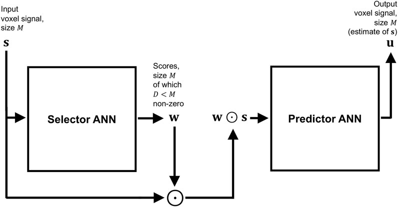
FIGURE 1. Block diagram summarising the architecture of SARDU-Net, made of two fully-connected ANNs that are optimised jointly end-to-end to find optimal subsets of measurements within lengthy quantitative MRI acquisitions. The first ANN is a selector: it takes as input a signal made of multiple MRI measurements from a voxel, and outputs a corresponding set of scores, which nullify non-salient measurements effectively extracting a subset of the fully-sampled signal. The second ANN is a predictor: it aims to retrieve the fully-sampled signal from the subset received from the selector.

Both selector and predictor are constructed as multi-layer, fully-connected feedforward ANNs, where each layer is obtained as a linear matrix operation followed by element-wise Rectified Linear Units (ReLU). Additionally, the activations of the selector output neurons are normalised to add up to one via softmin normalisation, and then thresholded so that only the $D$ top-firing neurons are kept. The remaining $M-D$ neurons are zeroed, so that the output scores $\mathbf{w}$ effectively select $D$ measurements. The activations of the selector output neurons are positive continuous numbers. The thresholding stage identifies which $D$ out of $M$ neurons to keep (i.e., the top firing), binarising the activations and selecting $D$ out of $M$ qMRI measurements. The selector and predictor are optimised jointly end-to-end to find a subset of measurements that carries the most information about the fully-sampled signal. For this, a loss function

$\mathit{L}= \Vert \mathbf{u}\left(\mathbf{w}\mathrm{o}\cdot \mathbf{s}\right)-\mathbf{s}\Vert { }_2^2(2)$

measuring the ${\ell }^2$-norm of the reconstruction error (i.e., mean squared error (MSE)) is minimised via back-propagation [46] with ADAM optimisation [47] and dropout regularisation [48]. In practice, the differentiable product $\mathbf{w}\mathrm{o}\cdot \mathbf{s}$ enables the propagation of error gradients from the predictor to the selector, and hence their joint optimisation.

For network training, input voxels intensities are normalised as

$\widehat{\mathbf{s}}= \frac{\mathbf{s}- {\mathit{s}}_{\text{min}}}{ {\mathit{s}}_{\text{max}}- {\mathit{s}}_{\text{min}} },(3)$

where $s_{\text{min}}= {10}^{-6}$ and $s_{\text{max}}$ is the 99th percentile of the range of variation of the signal intensity across the whole input set. Afterwards, voxels are split at random into actual training and validation sets. Training voxels are grouped and passed through the network in mini-batches; during one such forward network pass, the selector’s output neuron activations are averaged over the mini-batch before computing $\mathbf{w}$, and network parameters then updated. The whole set of training voxels is the input to the system for a fixed number of epochs, during which the loss function is evaluated on both training and validation set. In the latter case, the selector ANN is temporarily deactivated and the scores $\mathbf{w}$ are fixed to the latest values provided by training. The concatenation of a selector and a predictor network is trained end-to-end by backpropagating fully-sampled signal prediction errors through the predictor and then back through the selector.

Brain MRI

Acquisition

We performed brain DRI scans on three healthy volunteers (2 females, 1 male) using a 3T Philips Ingenia CX system. DRI featured joint diffusion-/T1-weightings, achieved by varying diffusion weighting and inversion time TI [17]. A multi-slice saturation inversion recovery (SIR) [49] DW EPI sequence was used, with the vendor’s 32-channel head coil for reception. Salient sequence parameters were: 48 axial-oblique slices, 2.4 mm-thick; field-of-view: 230 × 230 mm²; in-plane resoluton: 2.4 × 2.4 mm²; repetition time TR = 2,563 ms; TE = 90 ms; saturation delay TS = 300 ms; SENSE factor: 2; multiband factor: 3; readout bandwidth: 2.51 KHz/pixel. Scans were performed with 32 unique (b,TI) values among b = (0, 1000, 2000, 3000) s/mm² × TI = (70, 320, 570, 820, 1070, 1320, 1570, 1820) ms. For each (b,TI) pair, three images were acquired for b = 0 and 21 isotropic-distributed gradient directions for non-zero b-values, optimising directional distribution across the 3 b-shells according to [50]. This corresponded to 528 EPI images in total, with scan time of 45 min:12 s (MRI parameters in Supplementary Table S1). Additionally, one b = 0 image with reversed phase encoding direction was acquired for distortion correction.

Post-processing

Brain scans were denoised with Marchenko-Pastur Principal Component Analysis (MP-PCA) [51] (kernel: 5 × 5 × 5 voxels) and noise floor mitigated with a custom-written Matlab (The MathWorks, Inc., Natick, Massachusetts, United States) implementation of the method of moments [52]. Afterwards, motion and eddy current distortions were mitigated via affine co-registration based on NiftyReg (http://cmictig.cs.ucl.ac.uk/wiki/index.php/NiftyReg), with each volume co-registered with reg_aladin to the mean of all 528 EPI images. Finally, FSL topup [53] and bet [54] were used to mitigate EPI distortions and segment the brain. The median signal across all voxels and measurements was used to re-scale image intensities prior to downstream processing.

Experiments

We studied the ability of SARDU-Net to select informative sub-protocols within the set of DRI measurements. We followed a leave-one-out approach and used two out of three subjects to train a SARDU-Net in turn. The remaining subject was then used to test whether SARDU-Net selected an informative sub-protocol. For this demonstration we focussed for simplicity on (b,TI) sub-protocols, and did not consider gradient direction dependence, as in related literature [29]. We fed SARDU-Net with directionally-averaged DW signals [55] at fixed (b,TI), which are commonly referred to as powder-averaged or spherical mean signals. Directional averaging provides measurements that are not confounded by the underlying fibre orientation distribution [56], and is a common step in several DW MRI techniques [57–59].

SARDU-Net Training

Sub-protocols of $D=\{16, 8, 4\}$ out of $M=32$ measurements were searched, training a SARDU-Net for 300 epochs with the following parameters: 80 and 20% of voxels as training/validation sets; four hidden layers for selector ANN with $\{32,28,20,28,32\}$ neurons for $D=16$, $\{32,26,20,14,32\}$ for $D=8$, $\{32,25,18,11,32\}$ for $D=4$; architecture of the predictor mirroring that of the selector; 18 different sets of learning options within mini-batch size $=\{100, 800, 1500\}$ voxels × learning rate $=\{{10}^{-4}, {10}^{-3}\}$ × dropout regularisation $=\{0.0, 0.2, 0.4\}$. We used four hidden layers for both selector and predictor to obtain a total of 8 layers, as in preliminary tests this minimised the validation loss while also avoiding overfitting over a long epoch range (Supplementary Figure S3). The number of neurons was linearly decreased layer-by-layer from $M$ to $D$ for the selector, while it was increased from $D$ to $M$ for the predictor (note that $M-D$ non-selected measurements are zeroed in the selector input/predictor output). Training was performed 8 times for each learning option configuration, initialising the ANNs randomly each time to assess reproducibility. The performance of SARDU-Net sub-protocols in multi-contrast analyses (see below) was assessed using sub-protocols providing the lowest validation loss.

Multi-Contrast Analysis

We adapted a previous approach [60], which modelled brain white matter inversion recovery DW measurements at b-value $b$, gradient direction $\mathbf{g}$, inversion time $\text{TI}$ as

$\mathit{s}\left(\mathit{b}, \text{TI},\mathbf{g}\right)= s_0\left| {\displaystyle \sum }_{i=1}^{N_f}{v}_i \left(1-2 e^{- \frac{\text{TI}}{T_{1i}}}\right) e^{-b {\mathbf{g}}^{\text{T}}{\mathbf{D}}_i\mathbf{g}} \right|.(4)$

Above $v_i$, $T_{1i}$ and ${\mathbf{D}}_i$ are the volume fraction, longitudinal relaxation time and cylindrically-symmetric diffusion tensor of fibre population $i=1, \dots , N_f$. Here we adapted Eq. 4 by 1) including the effect of the saturation pulse (fixed saturation-inversion delay, TS = 300 ms); 2) considering directionally-averaged signals; 3) setting $N_f=1$ to deploy the model across the whole parenchyma, obtaining

$\mathit{s}\left(\mathit{b}, \text{TI},\text{ TS}\right)= \frac{\sqrt{\pi }}{2} s_0 \left| 1 - e^{- \frac{\text{TI}}{T_1}} - \left(1-e^{- \frac{\text{TS}}{T_1}} \right)e^{- \frac{\text{TI}}{T_1}} \right| e^{-b{d}_{\perp }} \frac{ \text{erf}\left( \sqrt{b(d_{\parallel }- d_{\perp })} \right) }{\sqrt{b(d_{\parallel }- d_{\perp })}} .(5)$

We refer to Eq. 5 as T1-weighted spherical mean diffusion tensor (T1-SMDT) model (the explanation of all terms in Eq. 5 is reported in the Appendix A1), with tissue parameters: $s_0$ (apparent proton density), $d_{\parallel }$ (fibre parallel diffusivity), $d_{\perp }$ (fibre perpendicular diffusivity), $T_1$ (relaxation time). $d_{\parallel }$ and $d_{\perp }$ map properties that are independent of the underlying fibre orientation distribution, and a per-fibre anisotropy index (${\text{AI}}_f$) can be derived [56] as

${\text{AI}}_f= \frac{d_{\parallel }}{d_{\perp }}.(6)$

We fitted the T1-SMDT model to the full set of (b,TI) measurements using a recent ANN-based fitting approach [61], as available in the qMRI-Net toolbox [62] (link: http://github.com/fragrussu/qMRINet; details in Supplementary Table S2). For comparison, we repeated T1-SMDT fitting for SARDU-Net sub-protocols as well as for sub-protocols obtained by uniform and geometric [63, 64] downsampling of the (b,TI) space.

Finally, we performed an extensive numerical evaluation in Matlab to assess SARDU-Net sub-protocols for their ability to inform downstream multi-contrast analyses for which they were not explicitly optimised. We compared SARDU-Net and uniform/geometric sub-protocols against 300 random unique sub-protocols of the same size in a dictionary-based model fitting experiment. We generated ∼400,000 synthetic signals for each SARDU-Net, naïve uniform and random sub-protocols of the same size by varying tissue parameters ($s_0$, $d_{\parallel }$, $d_{\perp }$, $T_1$) of Eq. 4 within a uniform grid. Afterwards, we obtained the combination of tissue parameters providing the lowest signal MSE, and used it to synthesise fully-sampled signals in each voxel. These were compared to the actual fully-sampled measured signals, obtaining voxel-wise MSEs which were averaged within one brain slice passing through the corpus callosum and containing all tissue types. Moreover, the mean value of the difference between each parameter map obtained from a sub-protocol and that obtained from the fully-sampled signal was also calculated. The closest quantile of the random protocol distribution to which the observed MSEs and parametric map differences (in absolute value) corresponded were also recorded for all of SARDU-Net, uniform and geometric sub-samplings.

Prostate MRI

Acquisition

We acquired in vivo DRI scans on three healthy males as part of an ongoing study [65] using a 3T Philips Achieva system. DRI featured different diffusion-/T2-weightings, achieved by varying b-value and echo time TE. A multi-slice diffusion-weighted (DW) echo planar imaging (EPI) sequence was used, with the vendor’s 32-channel cardiac coil for reception. Salient parameters were: 14 axial slices, 5 mm-thick; field-of-view of 220 × 220 mm²; in-plane resolution of 1.75 × 1.75 mm²; repetition time TR = 2,800 ms; SENSE factor: 1.6; half-scan factor: 0.62; 2 averages; 1 coronal REST slab for spatial saturation; readout bandwidth: 2.39 KHz/pixel. Scans were performed with 16 unique (b,TE) values among b = (0, 500, 1000, 1500) s/mm² × TE = (55, 87, 121, 150) ms. For each (b,TE), three images were acquired, using three orthogonal diffusion gradients when b was not zero, for a total of 48 DRI images (total scan time of 6 min:15 s; MRI parameters in Supplementary Table S3).

Post-processing

Prostate scans were denoised slice-by-slice with MP-PCA [51] (kernel: 7 × 7 voxels), and noise floor mitigated with the method of moments [52]. Motion and eddy current distortions were mitigated slice-by-slice by co-registering each 2D image to a reference with affine registration. NiftyReg reg_aladin was used, and the reference was obtained as the average of all volumes. Finally, the three images at any fixed (b,TE) obtaining 16 unique (b,TE) volumes, which were normalised by dividing by the median signal across all volumes and voxels within the prostate (same normalisation factor for all volumes). For this, a prostate mask was manually segmented on the mean EPI image calculated after co-registration in FSLView [66].

Experiments

Measurement subsets selected by SARDU-Net were tested for their potential of informing downstream tissue parameter estimation, as for example via HM-MRI [40, 41]. As in to brain DRI experiments, we followed a leave-one-out approach and used two out of three subjects to train a SARDU-Net in turn. The remaining subject was then used to test the SARDU-Net sub-protocol.

SARDU-Net Training

For each leave-one-out fold, measurements from prostate voxels of the two training subjects were extracted and assigned at random to training (80% of voxels) and validation (20% of voxels) sets. Sub-protocols of $D=\{12, 9\}$ out of $M=16$ measurements were searched by training a SARDU-Net for 300 epochs. Four hidden layers were used for selector/predictor ANNs (selector: $\{16, 15, 14, 13, 16\}$ neurons for $D=12$ and $\{16, 14, 13, 11, 16\}$ for $D=9$; predictor architecture mirroring selector), and 18 different sets of learning options (mini-batch size $=\{100, 800, 1500\}$ voxels × learning rate $=\{{10}^{-4}, {10}^{-3}\}$ × dropout regularisation $=\{0.0, 0.2, 0.4\}$). As for brain MRI, we used four hidden layers for selector/predictor to obtain a total of 8 layers, with the number of hidden neurons being linearly decreased layer-by-layer. Moreover, for each configuration of learning options, training was repeated 8 times using different random network initialisation seeds to assess reproducibility. For assessing the performance of SARDU-Net sub-protocols in multi-contrast analyses (see below), we used sub-protocols provided by the trained net with lowest validation loss.

Multi-Contrast Analysis

SARDU-Net measurement subsets were evaluated for their potential to inform multi-contrast signal analyses. For this evaluation, we adopted one among several potential methods in the literature, i.e., the HM-MRI [41] model, a multi-exponential approach describing the total prostate signal as the sum of luminal, epithelial and stromal components:

$s\left(b,\text{TE}\right)= s_0 \left(v_l e^{-b d_l - \frac{\text{TE}}{T_{2l}} }+\left(1- v_l\right) \left(v_e e^{-b d_e - \frac{\text{TE}}{T_{2e}} }+ \left(1- v_e\right) e^{-b d_s - \frac{\text{TE}}{T_{2s}} }\right(\right(.(7)$

In Eq. 7, $s\left(b,\text{TE}\right)$ is the prostate signal at a fixed $b$-value and echo time $\text{TE}$. The 9 tissue parameters are: $s_0$ (apparent proton density); $v_l$ (luminal water voxel volume fraction); $v_e$ (epithelial fraction of non-luminal tissue); $d_l$, $d_e$, $d_s$ and $T_{2l}$, $T_{2e}$, $T_{2s}$ (ADC and T2 of luminal/epithelial/stromal water).

Firstly, HM-MRI metrics were computed on the fully-sampled scans and on SARDU-Net and on naïve sub-protocols ($D=\{12, 9\}$) for comparison, with sub-protocols obtained by uniform and geometric [63, 64] downsampling of the (b,TE) measurement space. We used the same ANN-based fitting procedure used for brain DRI [62] and estimated voxel-wise $v_l$, $v_e$ and $s_0$, while fixing compartment-wise ADC and T2 values to literature values [41] (details in Supplementary Table S4).

Subsequently, we assessed the potential of SARDU-Net sub-protocols to enable downstream analyses for which they were not explicitly optimised for. We performed a similar dictionary-based fitting experiment in Matlab as done for brain DRI (Experiments, Multi-contrast analysis). In this case, we restricted our analysis to the central slice of each prostate and synthesised a database of ∼125,000 reference signals for each $\left(\begin{array}{c}M\\ D\end{array}\right)= \frac{M!}{\left(M-D\right)! D!}$ subset of $D=\{12, 9\}$ out of $M=16$ measurements (1,820 for $D=12$; 11,440 for $D=9$) by varying tissue parameters uniformly on a grid of previously reported values [41]. The combination of parameters providing the lowest sub-protocol MSE was used to synthesise fully-sampled signals and then compute the average mean squared error (MSE) for the fully-sampled protocols within the region-of-interest. As for the brain data, the mean value of the difference between each parameter maps obtained from a sub-protocol and from the full protocol was recorded. Finally, the distributions of MSE and parameter map differences from the whole set of $\left(\begin{array}{c}M\\ D\end{array}\right)$ sub-protocols were used to assess to which quantile each of SARDU-Net, uniform and geometric figures corresponded to.

For all analyses, computation was run on a 24-core 2.8 GHz AMD Opteron(tm) 6,348 Processor CPU, running CentOS Linux 7 (Core).

Results

Brain MRI

Figure 2 shows SARDU-Net selection of $D=\{16,8,4\}$ out of $M=32$ (b,TI) measurements on brain DRI from training fold 1 (complete list of measurement selection available in Supplementary Table S5; examples of sub-protocol selection during training available in Supplementary Figure S1). SARDU-Net sub-protocols sample the full range of b and TI values. However, they sample less densely measurements characterised by the lowest signal-to-noise ratio (SNR) levels, as for example strong diffusion-weightings for TI close to the SIR null point.

FIGURE 2

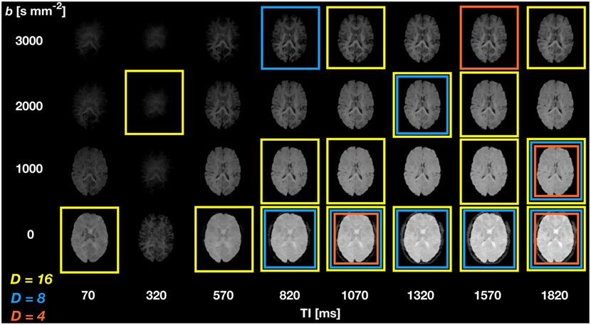
FIGURE 2. SARDU-Net measurement selection on DRI of the brain. The figure illustrates results from leave-one-out fold 1 (subject 1 left out during training, which is performed on subjects 2 and 3) for selection of $D=16$ (yellow boxes), and $D=8$ (blue boxes) and $D=4$ (orange boxes) out of $M=32$ (b,TI) measurements. The images show spherical mean signals form one brain slice of subject 1. Inversion times (TI, delay between inversion pulse and slice excitation) are arranged along different columns, while diffusion-weightings (b) along different rows. The saturation delay TS (i.e., delay between saturation pulse and inversion pulse) is fixed for all (b,TI) measurements to TS = 300 ms.

Figure 3 shows SARDU-Net reproducibility on brain DRI. Results from different sub-sampling factors are shown in different rows, while results from different leave-one-out training folds are shown in different columns. SARDU-Net measurement selection is consistent across different algorithm initialisations and different training folds. A number of measurements are selected consistently in all cases [e.g., (b,TI) = (0 s mm⁻²; 1800 ms)], while other measurements [e.g., (b,TI) = (1,000 s mm⁻²; 70 ms)] are avoided consistently.

FIGURE 3

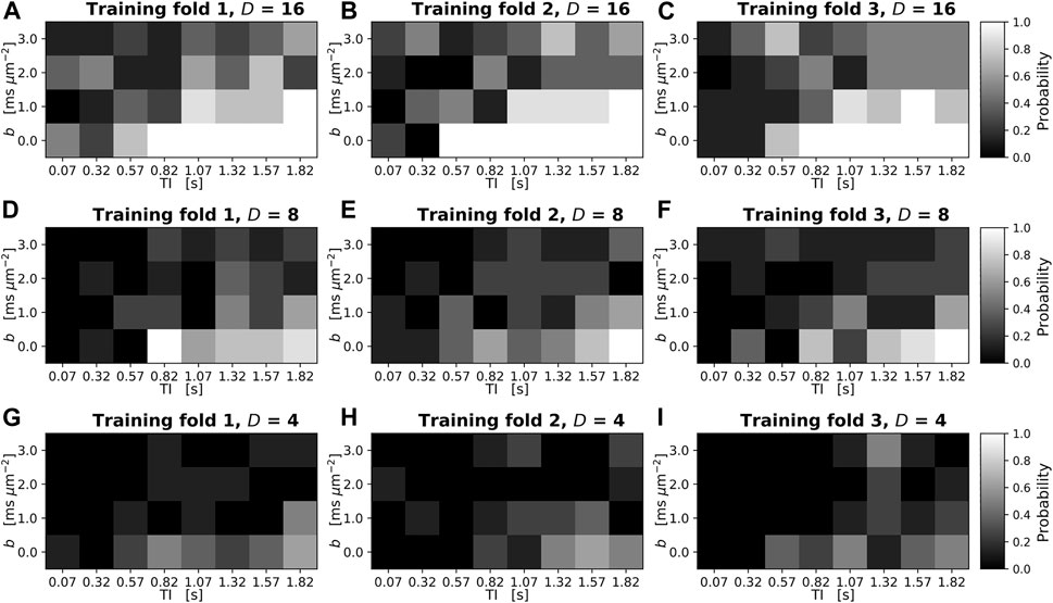
FIGURE 3. Reproducibility of SARDU-Net measurement selection for in vivo brain DRI over different leave-one-out training folds and random initialisations. The normalised 2D histogram in each panel shows the probability of each (b,TI) measurement being selected over eight different repetitions of the SARDU-Net training. Each repetition featured a unique random initialisation of the SARDU-Net parameters, with all other training options (i.e., mini-batch size, dropout regularisation, learning rate) fixed to the configuration providing the lowest validation loss. Panels (A–C) (top row): selection of $D=16$ out of $M=32$ measurements (A, left: subject 1 out during training and used for testing; B, middle: subject 2 left out; C, right: subject 3 left out). Panels (D–F) (middle row): selection of $D=8$ measurements (D, left: subject 1 out; E, middle: subject 2 out; F, right: subject 3 out). Panels (G–I) (bottom row): selection of $D=4$ measurements (G, left: subject 1 out; H, middle: subject 2 out; I, right: subject 3 out).

Table 1 reports subject-wise signal MSE and mean brain T1-SMDT map differences with respect to maps obtained from fully sampled signals. The table also reports 95% ranges from the random sub-protocol distribution, and the quantile of such a distribution to which SARDU-Net, uniform and geometric sub-sampling figures correspond to. For all sub-sampling factors, SARDU-Net sub-protocols ensure a better signal reconstruction (i.e., lower MSE) based on the T1-SMDT model as compared to uniform and geometric sub-sampling. For 2 subjects out of 3, SARDU-Net-based MSE is also within the lowest 5% of the random protocol distribution, being higher in just two cases (9 and 12% for subject 2, $D=16$ and $D=8$). Among SARDU-Net, uniform and geometric sub-sampling, SARDU-Net sub-protocols enable the computation of maps that are the closest to those obtained from fully sampled signals for $T_1$ and $s_0$ for strong sub-sampling factors ($M=4$). For less strong sub-sampling factors and for parametric maps $d_{\parallel }$ and $d_{\perp }$, there is not a sub-sampling strategy that consistently enables the reconstruction of parametric maps that are the closest to full sampling. Finally, in most cases SARDU-Net, uniform and geometric sub-samplings lead to the computation of parametric maps whose difference with respect to reference metrics lies in the interquartile range of the random sub-protocol distribution.

TABLE 1

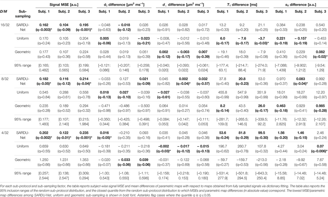
TABLE 1. Results of the SARDU-Net, uniform and geometric sub-protocol comparison against a null distribution from randomly selected sub-protocols (brain data, T1-SMDT model).

Figure 4 shows T1-SMDT reference parametric maps from the full protocol as well as those derived from sub-protocols. On visual inspection, parametric maps derived from SARDU-Net, uniform and geometric sub-protocols are comparable to the reference when half of the measurements are kept in the sub-protocol ($D=16$ out of $M=32$ measurements). However, for stronger downsampling ($D=8$ and $D=4$), SARDU-Net and geometric sub-protocols preserve key between-tissue contrasts in all parametric maps, unlike uniform sub-protocols.

FIGURE 4

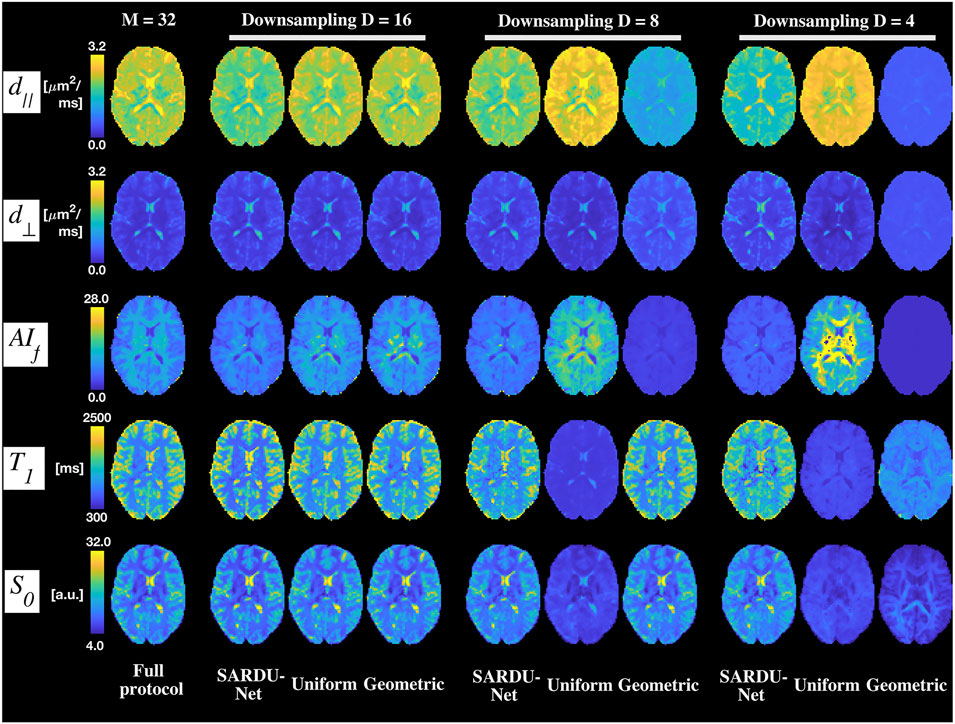
FIGURE 4. Examples of brain T1-SMDT parametric maps. Different rows show T1-SMDT metrics, while different columns refer to different protocols. From left to right: full protocol; SARDU-Net, uniform and geometric subprotocols for $D=16$, $D=8$ and $D=4$ measurements. Uniform sub-protocols are: (b,TI) = (0, 1000, 2000, 300) s mm⁻² × (70, 570, 1070, 1570) ms for $D=16$; (b,TI) = (0, 1000, 2000, 300) s mm⁻² × (70, 1070) ms for $D=8$; (b,TI) = [(0, 70), (2000, 70), (1000, 1070), (3000, 1070)] (s mm⁻², ms) for $D=4$. Geometric sub-protocols are: (b,TI) = (0, 1000, 2000, 300) s mm⁻² × (70, 320, 820, 1820) ms for $D=16$; (b,TI) = (0, 2000) s mm⁻² × (70, 320, 820, 1820) ms for $D=8$; (b,TI) = [(1000, 70), (0, 320), (2000, 820), (3000, 1820)] (s mm⁻², ms) for $D=4$.

Prostate MRI

Figure 5 shows SARDU-Net selection of $D=12$ and $D=9$ out of $M=16$ prostate measurements. The figure refers to training fold 1, with the complete list of measurement selection for all folds in Supplementary Table S6. Additionally, an example of the evolution of sub-protocol selection during training is included as Supplementary Figure S2. Figure 6 demonstrates that SARDU-Net sub-protocols sample the full range of diffusion and relaxation weightings. While measurements with the lowest SNR levels (i.e., maximum b and longest TE) are generally not kept in SARDU-Net sub-protocols, in some cases measurements that are selected by SARDU-Net feature lower SNR than measurements that are not selected (e.g., for $D=9$, (b,TE) = (1,500 s mm⁻², 87 ms) is kept, while (b,TE) = (500 s mm⁻², 87 ms) is not).

FIGURE 5

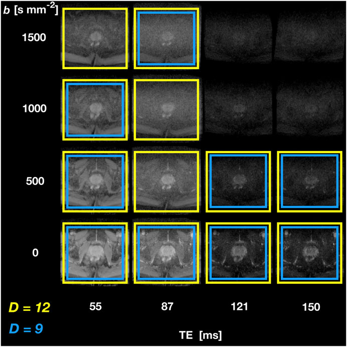
FIGURE 5. SARDU-Net measurement selection on DRI of the prostate. The figure illustrates results from leave-one-out training fold 1 (subject 1 left out during training, which is performed on subjects 2 and 3) for selection of $D=12$ (yellow boxes) and $D=9$ (blue boxes) out of $M=16$ (b,TE) measurements. Echo times (TE) are arranged along different columns, while diffusion-weightings (b) along different rows.

FIGURE 6

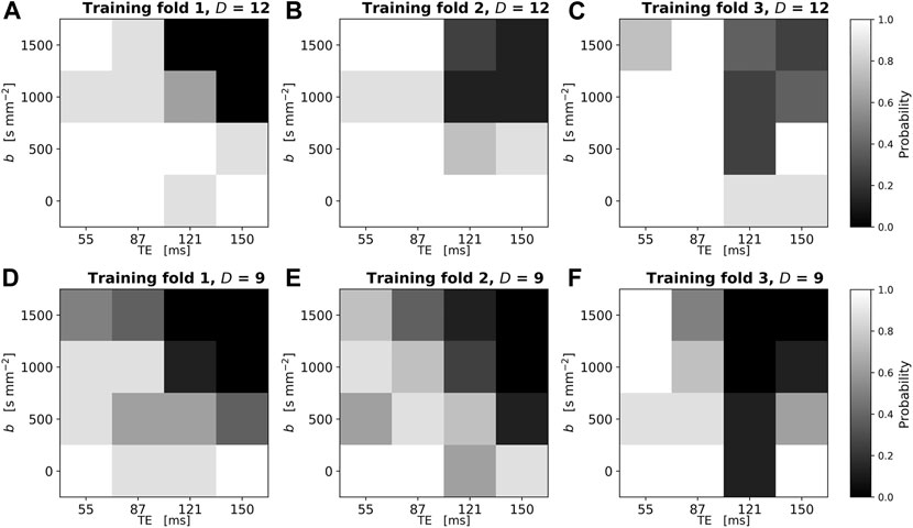
FIGURE 6. Reproducibility of SARDU-Net measurement selection for in vivo prostate DRI over different leave-one-out training folds and random initialisations. The normalised 2D histogram in each panel shows the probability of each (b,TE) measurement being selected over eight different repetitions of the SARDU-Net training. Each repetition featured a unique random initialisation of the SARDU-Net parameters, with all other training options (i.e., mini-batch size, dropout regularisation, learning rate) fixed to the configuration providing the lowest validation loss. Panels (A–C) (top row): selection of $D=12$ out of $M=16$ measurements (A, left: subject 1 left out during training and used for testing; B, middle: subject 2 out; C, right: subject 3 out). Panels (D–F) (bottom row): selection of $D=9$ measurements (D, left: subject 1 out; E, middle: subject 2 out; F, right: subject 3 out).

Figure 6 shows the reproducibility of SARDU-Net sub-protocol selection across 8 different random initialisations in each training fold. Each panel reports as a 2D histogram the normalised count of each (b,TE) measurement being selected over the 8 different random seeds (top row: $D=12$; bottom row: $D=9$; different folds along different columns). The illustrations demonstrate that SARDU-Net sub-protocol selection is consistent across leave-one-out folds and random initialisations. For instance, the same 8 measurements out of 12 were consistently selected in all 8 random training repetitions for $D=12$ in fold 2 and 3, while in no cases SARDU-Net selected the measurement corresponding to sequence parameters (b,TE) = (1,500 s mm⁻²,150 ms).

Table 2 reports subject-wise signal MSE and mean prostate HM-MRI map differences with respect to maps obtained from fully sampled. The table also reports 95% ranges from the all sub-protocol distribution, and the quantile of such a distribution to which SARDU-Net, uniform and geometric sub-sampling figures correspond to. For all sub-sampling factors, SARDU-Net sub-protocols ensure a better signal reconstruction (i.e., lower MSE) based on the HM-MRI model as compared to uniform and geometric sub-sampling. In all cases, SARDU-Net sub-protocols lead to an MSE that is within the lowest 6% of the distribution from all $\left(\begin{array}{c}M\\ D\end{array}\right)$ sub-protocols. SARDU-Net sub-protocols also enable the computation of parametric maps that in most cases show smaller differences (in absolute value) to metrics derived from fully-sampled signals as compared to uniform and geometric sub-sampling. The differences are in most cases within the lowest quartile of the distribution from all possible $\left(\begin{array}{c}M\\ D\end{array}\right)$ sub-protocols.

TABLE 2

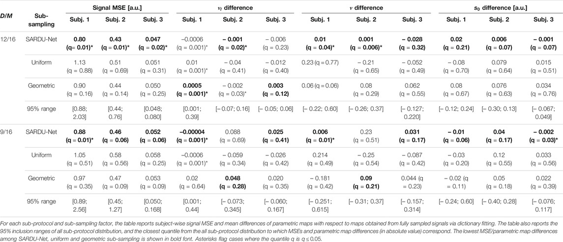
TABLE 2. Results of the SARDU-Net, uniform and geometric sub-protocol comparison against a null distribution obtained from all possible sub-protocols (prostate data, HM-MRI model). The bold font indicates the lowest MSE/lowest parametric map difference among values obtained for SARDU-Net, uniform and geometric sub-samplings.

Figure 7 illustrates examples of HM-MRI indices obtained on the full protocols as well as on SARDU-Net, uniform and geometric sub-protocols. Regional variation of $v_l$ and $v_e$ maps is in line with known anatomy of the healthy prostate, as for example increased luminal water fraction in the peripheral zone. On visual inspection, metrics obtained from both SARDU-Net, uniform and geometric sub-protocols show within-prostate contrasts that are qualitatively similar to those obtained from the full protocols. HM-MRI metrics from SARDU-Net sub-protocols appear closer to the fully-sampled reference than other sub-protocols.

FIGURE 7

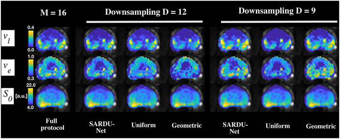
FIGURE 7. Examples of prostate HM-MRI parametric maps. Different rows show HM-MRI metrics, while different columns refer to different protocols. From left to right: full protocol; SARDU-Net, uniform and geometric subprotocols for $D=12$ and $D=9$ measurements. Uniform sub-protocols were: (b,TE) = (0, 500, 1000, 1500) s mm⁻² × (55, 121, 150) ms ($D=12$); (b,TE) = (0, 1000, 1500) s mm⁻² × (55, 121, 150) ms ($D=9$). Geometric sub-protocols were: (b,TE) = (0, 500, 1500) s mm⁻² × (55, 87, 121, 150) ms ($D=12$); (b,TE) = (0, 500, 1500) s mm⁻² × (55, 87, 150) ms ($D=9$).

Discussion

Key Findings

This paper investigates the feasibility of data-driven, model-free qMRI experiment design based on the analysis of lengthy pilot in vivo scans. Such scans were analysed with an ANN-based method, SARDU-Net, which identifies informative sub-protocols to facilitate the deployment of the latest qMRI techniques in contexts where scan time is limited. Our main finding is that identifying informative sub-protocols within in vivo pilot scans without relying on explicit parametric, biophysical signal models is feasible, and that SARDU-Net provides a general, robust and reproducible procedure to identify such sub-protocols, showing utility across a range of anatomical districts (e.g., brain, prostate) and contrasts (diffusion, T2, T1).

Sub-protocol Selection

We studied DRI scans of the brain and prostate acquired at 3T on two separate groups of healthy volunteers. Brain scans consisted of 32 unique (b,TI) measurements via SIR DW imaging, while prostate scans featured 16 unique (b,TE) measurements. Data were analysed with SARDU-Net to identify informative sub-protocols within the fully-sampled measurement set, made of 16, 8 and 4 out of 32 for brain and 12 and 9 measurements out of 16 for prostate. The reproducibility of the measurement selection procedure across leave-one-out folds and random initialisations was also assessed.

Our results demonstrate that data-driven, model-free protocol selection methods such as SARDU-Net identify informative sub-protocols within densely sampled measurement sets, and that such sub-protocols do not necessarily feature uniform downsampling of the acquisition space. The selected measurements span the whole range of signal weightings for both brain and prostate. Nonetheless, measurements with the lowest SNR levels (i.e., maximum b and TI close to neural tissue SIR null point; maximum b and longest TE for prostate DRI) are consistently avoided. This suggests that noise is an important factor to consider for qMRI sampling design. While model-based optimisation typically relies on some a priori hypotheses on the level and statistics of thermal noise, our fully-data driven approach enables the design of qMRI samplings from real-world SNRs and noise distributions. Moreover, in this pilot investigation we did not focus on the angular dependence of the diffusion signal, and therefore treated all (b,TI) (for brain) and (b,TE) (for prostate) contrasts equally. Nevertheless, in real-life scenarios some contrasts may be much cheaper to acquire than others (e.g., a b = 0 image is much faster to acquire than a full b-shell at non-zero b), and could therefore be included in the final qMRI sub-protocol in any case, even if not selected by the algorithm. Also, the measurement selection algorithm could be adapted to account for the difference in acquisition time needed for b-shells of different size and/or b = 0 images, e.g., by weighting scores attached to each b-shell by their cost in terms of acquisition [67].

We also characterised the reproducibility of SARDU-Net. Results from both brain and prostate demonstrate that the stability of our sub-protocol selection procedure can enable practical protocol design from a limited number of pilot scans. However, our results also highlight that some variation in sub-protocol selection across training folds ad random algorithm initialisations. The former is likely to originate from intrinsic between-subject variability, and could be minimised by ensuring that the pilot training cohort is large enough to capture biological variability. The latter suggests the presence of different local minima in the algorithm loss function, a known issue in optimisation problems. Such latter variability appears to be small, since a number of key information-carrying measurements are selected consistently. However, in future we aim to reduce the sensitivity of the training procedure to the initial conditions.

Multi-Contrast Analysis

We tested sub-protocols selected by SARDU-Net for their ability to inform downstream model-based multi-contrast analyses, for which they were not optimised explicitly. To this end, we adapted a previous brain white matter modelling method to our SIR DWI data (i.e., here referred to as T1-SMDT), and utilised a simple multi-exponential model capturing the joint (b,TE) dependence of the MRI signal in the prostate (i.e., the HM-MRI model). Both models were fitted to the full set of measurements and on sub-protocols provided by SARDU-Net, as well as on uniform and geometric sub-sampling of the measurement space. On visual inspection, parametric maps obtained from SARDU-Net sub-protocols are closer to reference maps from full protocols, especially in the brain and when downsampling is stronger, suggesting that SARDU-Net sub-protocols preserve key features of measured signals.

Importantly, parametric maps from both HM-MRI and T1-SMDT models exhibit differences when derived from different DRI protocols. This highlights the intrinsic challenge of inverting highly non-linear models to resolve diffusion/relaxation properties from noisy measurements [8, 68]. Importantly, we point out that the HM-MRI and T1-SMDT models were simple and convenient choices for our demonstration. Different approaches within a wider landscape of alternative models could have been equally adopted, each with its own advantages and disadvantages. In particular, VERDICT [7] and Relaxed-VERDICT [69] would account for diffusion time in prostate DRI, neglected in this study, while multi-compartment models [8, 58, 70, 71] could be adapted for brain DRI. We reserve such alternative approaches for future investigation.

Finally, we compared SARDU-Net sub-protocols for their ability to capture salient characteristics of input MRI signals against an extensive list of alternative sub-protocols. We used the T1-SMDT and HM-MRI models to reconstruct fully-sampled signals from 1) all possible sub-protocols of fixed size for prostate DRI (12 and 9 measurements out of 16) and from 2) 300 random sub-protocols for brain DRI (16, 8 and 4 measurements out of 32), as well as from SARDU-Net, uniform and geometric downsampling. Our analyses show that SARDU-Net sub-protocols capture salient features of fully-sampled DRI signals, since in almost all cases they are within the top-performing (best 5%) sub-protocols in terms of reconstruction MSE, hence approximating the best small-sample/task-specific protocols without being trained specifically to do so. Also, Figures 4, 7 as well as Tables 1, 2 show that parametric maps from SARDU-Net sub-protocols are good approximations of reference metrics from fully-sampled signal. Nevertheless, they are not the closest to the reference maps, despite being the signal MSE (i.e., a measure of the quality of fit) the lowest, as for example for $d_{\left|\right|}$ in brain MRI. This finding may be explained by considering that: 1) parameters such as $d_{\left|\right|}$ may be generally very difficult to estimate because of low sensitivity of the signal [68]; 2) different combinations of microstructural parameters may lead to similar MRI signal predictions and hence MSE; 3) the random protocols that score best on a specific parametric maps may be the best for this specific task and data set, whereas SARDU-net is designed in such a way as to be generically most informative. We point out that 2) can lead to ill-posed model inversion in quantitative MRI, i.e., to degenerate model fitting landscapes [68] such that a good quality of fit in signal space may not be a guarantee of accurate parameter estimation [72]. Regarding the accuracy in brain MRI parameter maps estimation (e.g., point 1) above for $d_{\left|\right|}$), we point out that SARDU-Net sub-protocol maps are less close to references for brain MRI than they are for prostate MRI. We speculate that this issue is seen more clearly in our brain data, rather than prostate data, since the model used in brain MRI has more tissue parameters than for prostate (T1-SMDT for brain, with four free parameters: $d_{\left|\right|}$, $d_{\perp }$, $T_1$, $s_0$; HM-MRI for prostate, with three free parameters: $v_l$, $v_e$, $s_0$. Note that in HM-MRI compartment-wise diffusivities and T2 relaxation times, notoriously difficult to fit [68], are fixed and not fitted. Regarding signal prediction, SARDU-Net MSEs are consistently lower than those provided by uniform/geometric uniform sub-protocols in both brain and prostate data, with the difference in performance becoming stronger as subsampling becomes more aggressive. This suggests that uniform sampling of DRI measurement spaces is a reasonable choice when a high number of measurements can be taken. However, non-trivial sampling is likely to capture salient signal characteristics better when only a few measurements can be taken. When the sub-sampling factor is not too strong (i.e., for moderate sub-sampling), simpler sub-sampling strategies (i.e., geometric/uniform sub-sampling) may work reasonably well. Therefore, data-driven sub-protocol selection approaches such as SARDU-Net may be most useful when very short acquisitions are to be searched within lengthy pilot protocols.

Finally, we remark once more that no information about parametric maps is used for SARDU-Net training: this is a deliberate design choice, as we aim to explore the potential of model-free protocol design. SARDU-Net sub-protocols are assessed during training for their ability to enable prediction of fully-sampled signals. Here we find that SARDU-Net sub-protocols do enable excellent fully-sampled signal predictions, even when an independent predictor (i.e., the T1-SMDT/HM-MRI models for brain/prostate) is used instead of the trained SARDU-Net predictor network. This demonstrates that SARDU-Net is an effective algorithm to identify measurements that carry information about the overall signal characteristics. Interestingly, SARDU-Net parametric maps are not necessarily the closest to references from fully-sampled signals. This is seen, for example, when comparing uniform and SARDU-Net sub-sampling for $D$/$M$ = 16/32, a task for which brain T1-SMDT parametric maps from SARDU-Net sub-protocols exhibit certain qualitative differences compared to references from fully-sampled signals. However, we also point out that in the same sub-sampling task the signal MSE from SARDU-Net sub-protocols is lower than for uniform sub-sampling, demonstrating that SARDU-Net training was successful in identifying a sub-protocol that supports optimal estimation of the full signal. We speculate that the measurements selected by SARDU-Net for the brain $D$/$M$ = 16/32 task may be prone to degeneracies of the fitting landscape [68, 72]. This could explain why the better quality-of-fit in terms of MRI signal for the SARDU-Net subprotocol does not translate to a higher accuracy in terms of parameter maps, as compared to uniform sub-sampling. Importantly, we highlight that for a specific choice of model, it is likely that a sub-protocol enabling the most accurate parameter map estimation could be found by optimising the Fisher matrix of the model itself [29]. SARDU-Net aims for a protocol that is generally the richest in information, independently of the choice of model. Our experiments verify this by showing that SARDU-Net sub-protocols enable optimal estimation of the full signal, and also perform well in estimating parameter maps for previously unseen models.

Methodological Considerations

Data-driven qMRI protocol design methods such as SARDU-Net would require the acquisition of a small number of rich, pilot qMRI scans when a new clinical study is being set up, from which informative sub-protocols could be identified given a scan time budget. Pilot scans are typically performed any way for quality control when developing new MRI procedures. Importantly, such pilot scans could be included in subsequent group-level analyses, since the final protocol would be a subset of it.

In this first explorative analysis, we tested data-driven protocol design on a small number of healthy volunteers, under the hypothesis that this suffices to capture the essence of DRI qMRI signals in brain and prostate, at least to demonstrate the potential of SARDU-net. Nonetheless, we acknowledge that including greater diversity of training data is important to enable the selection of qMRI protocols that capture key signal features, in particular including patient data to provide samples from pathological tissues we expect to observe in practice. Also, richer training data sets may lead more generalisable solutions, for instance by enabling a better characterisation of inter-subject variability. The choice of the training set remains a critical issue in general for machine learning-based approaches of this type; poor choices can lead to bias in many applications including qMRI, as demonstrated in [73, 74]. Such effects can affect data-driven protocol optimisation in a very similar way and future work will need to address this critical point to ensure responsible and reliable application of the method. We reserve the investigation of measurement selection in larger cohorts including both patients and controls to future applicative studies. These may exploit data augmentation techniques to increase the number of examples of under-represented pathological signals, as well as from any other tissue whose accurate characterisation may be of interest (e.g., grey matter compared to white matter).

Importantly, we point out that the latest acquisition technologies [15] make it achievable to sample two to four sequence parameters (e.g., echo time, inversion time and diffusion encoding) densely in under 1 h [17], as required in data-driven protocol optimisation approaches as SARDU-Net. However, data-driven optimisation would become impractical if larger acquisition spaces were of interest, as pilot protocols exceeding the hour would be needed. Related to this point, we acknowledge that our prostate DRI was well under the hour limit (nominal scan time of 6 min), and therefore may not be as representative of rich qMRI samplings as our brain DRI acquisition instead. This was due to the fact that the scan was performed as part of an ongoing MRI study [65]. In future, we will explore richer (b,TE) samplings and include diffusion time dependence [7, 69], which is not considered in this demonstration, to better assess the potential of SARDU-Net for prostate imaging.

We remark that our model-free approach is an alternative to previous model-based optimisation strategies [29], which remain valid options when a specific model is the main interest of a study. Here we report on a first exploratory analysis of the feasibility of an alternative framework, i.e., data-driven model-free qMRI protocol design. Model-based approaches make strong assumptions about the mathematical form of the signal and its relation to the underlying tissue, but do not require the acquisition of training data; data-driven approaches, on the other hand, do not make hypothesis on the explicit MRI signal parametrisation as a function of microstructural properties, but rely on the hypothesis that the available training data is representative. Such an alternative approach, with its own advantages and disadvantages, may be appealing when multiple downstream analyses are of interest or when the qMRI model is not known to a high degree of confidence at the time of the acquisition, a common situation in qMRI. Nevertheless, we acknowledge that future work is required to confirm the findings of this study before data-driven, model-free protocol design can be deployed in larger groups of healthy volunteers or patients.

Importantly, data-driven protocol design based on dense pilot scans, such as SARDU-Net, inevitably leads to discretising the acquisition parameter space, owing to the discrete sampling of the input scans, which is further sub-sampled in the sub-protocol search (Figures 3, 6). Such an approach requires the input qMRI protocol to be dense enough to capture the essence of the signal, i.e., that the resolution in sequence parameter space suffices to characterise its salient features (note that the output qMRI sub-protocol is necessarily a subset of the input measurement set). Moreover, we point out that the discretised acquisition space still supports, continuous, band-limited representations (e.g., expansions in spherical harmonic bases for the diffusion signal), which may offer complementary solutions for protocol optimisation to the ANN-based approach used here. This may prove especially useful when considering the angular dependence of the diffusion signal, which is not considered here, where all (b,TI) (for brain) and (b,TE) (for prostate) contrasts are treated equally as a first proof-of-concept. In future, we plan to compare our approach to alternative and equally valid frameworks based on continuous representations [75–77] or on the joint the application of dictionary learning and compressed sensing on simulated data [78].

Furthermore, in this work we compared sub-protocols selected by SARDU-Net to uniform and geometric downsamplings of DRI measurement spaces and, more generally, to a large number of randomly selected sub-protocols. We acknowledge that alternative uniform or geometric sub-samplings of the discrete input (b,TI) and (b,TE) measurement space could have been identified. We avoided trivial sub-protocols that would have provided unfair advantages to SARDU-Net (for instance, all b-values were included in uniform brain DRI sub-protocols even when $D=4$), and included computational experiments where SARDU-Net sub-protocols are compared to an exhaustive list of alternatives (300 sub-protocols for brain DRI; all sub-protocols for prostate DRI). In both cases SARDU-Net sub-protocols enable downstream analyses for which they were not explicitly optimised for, suggesting model-free methods such as SARDU-Net can capture the salient features of input MRI signals. Interestingly, testing the quality of signal/metric predictions for a number of randomly-selected sub-protocols may be per se an effective way of finding informative sub-samplings when exhaustive searchers are not tractable. However, these random protocol searches as implemented here are fundamentally distinct from SARDU-Net, since they relied on biophysical models of the MRI signal (i.e., T1-SMDT for brain; HM-MRI for prostate). Therefore, they do not represent an alternative model-free solution to SARDU-Net, but constitute a model-based optimisation strategy. Notably, SARDU-Net provided close to optimal solutions even for tasks for which it was not directly optimised for.

We showed the utility of coupling and optimising jointly a selector and a predictor. We demonstrated this by implementing both with fully-connected ANNs, given their excellent function approximation properties [79, 80]. This simple structure suffices to demonstrate the potential and flexibility of data-driven qMRI protocol design, making the algorithm easy to train with limited computational resources when extensive sub-protocols searches become unfeasible (i.e., a situation quickly reached for $M \sim 30$). Nonetheless, we acknowledge that different design choices could be equally valid, as for example genetic searches [33] for the selection stage. Also, at present we use the selector output neuron activations to decide on which measurements to include in the sub-protocols, effectively performing hard thresholding. We plan to explore more sophisticated selection strategies that could make use of the continuous information carried out by the selector output activations. We also plan to replace the simple grid search used here to design SARDU-Net learning options, and to explore alternative architectures beyond the four layers with linearly decreasing/increasing hidden neuron number used here (Supplementary Figure S3). Future work will extend sub-protocol selection to search for a trade-off between signal reconstruction quality (i.e., signal MSE) and scan time (i.e., sub-protocol size $D$), or to implement hybrid approaches that include information on the quality of parametric maps.

In this study, we used SARDU-Net as a tool to identify informative sub-protocols within lengthy pilot scan. Nonetheless, it should be noted that SARDU-Net effectively learns a mapping from a short qMRI protocol to a richer one. Therefore, one could potentially employ a trained SARDU-Net to enhance/enrich a qMRI protocol. Here we did not explore this application, since alternative architectures and/or learning strategies, specifically designed for this task [81], are likely to outperform SARDU-Net.

We also point out that SARDU-Net neither measures the SNR level of the input data, nor parametrises the sub-protocol selection as a function of SNR. SARDU-Net is a fully data-driven approach, and the sub-protocols that it identifies may therefore vary depending on the SNR of the input scans, for any fixed input sampling scheme. It follows that such output sub-protocols should be used for prospective acquisitions whose SNR is comparable to that of the data used for SARDU-Net training. Moreover, SARDU-Net does not model explicitly the dependence of the signal on the actual sequence parameter values, as it outputs a simple numbered list of selected measurements (e.g., measurement #0, #4, #9, etc). Departures from the nominal sequence parameter values may lead to the selection of different measurement sub-sets should such departures be strong enough to introduce new features in the fully-sampled signal.

Conclusions

The model-free, data-driven identification of economical but informative qMRI protocols for clinical application under high time pressure from a small number of rich pilot acquisitions with long acquisition times is feasible. For this purpose, approaches such as SARDU-Net offer practical solutions to identify sub-protocols that capture the salient characteristics of densely-sampled training MRI signals.

Data Availability Statement

The raw data supporting the conclusions of this article will be made available by the authors, without undue reservation.

Data and Code Availability Statement

Our open-source implementation of SARDU-Net is freely available online (permanent link: http://github.com/fragrussu/sardunet). All analysis scripts written for this paper will be made openly available online upon publication (permanent link: http://github.com/fragrussu/PaperScripts/tree/master/sardunet). These depend on the following third-party toolkits:

• FSL: http://fsl.fmrib.ox.ac.uk/fsl/fslwiki

• NiftyReg: http://cmictig.cs.ucl.ac.uk/wiki/index.php/NiftyReg

• MP-PCA: http://github.com/NYU-DiffusionMRI/mppca_denoise/blob/master/MPdenoising.m

• Noise-floor mitigation: https://github.com/fragrussu/MRItools/tree/master/matlabtools/MPio_moments.m

• Gibbs ringing removal: http://github.com/RafaelNH/gibbs-removal

• qMRI-Net: http://github.com/fragrussu/qMRINet

The diffusion gradient direction scheme for the in vivo brain data was generated with: http://www.emmanuelcaruyer.com/q-space-sampling.php.

Researchers interested in accessing the prostate MRI scans can contact Prof Daniel C. Alexander (d.alexander@ucl.ac.uk), while researchers interested in the brain MRI scans can contact Prof Claudia A. M. Gandini Wheeler-Kingshott (c.wheeler-kingshott@ucl.ac.uk). They will facilitate the stipulation of a data sharing agreement to access the data in fully anonymised form, enabling non-commercial research use will be stipulated.

Ethics Statement

The study was reviewed and approved by the London-Harrow Research Ethics Committee (05/Q0502/101) and by the London-Central Research Ethics Committee (16/LO/1440, ClinicalTrials.gov Identifier: NCT03151512). The participants provided their written informed consent to participate in this study.

Author Contributions

Conceptualisation: all authors. Algorithm and software development: FG, SB, HL, AI, TM, DCA. Data Acquisition: FG, MB, LK, TS, SS, DA, TM, RB. Data curation, formal analysis and visualisation: FG. Project administration: FG, TM, EP, DCA. Manuscript writing and editing: all authors. Funding acquisition: SP, DA, RB, CWK, EP, TM, DCA.

Funding

This project was funded by the Engineering and Physical Sciences Research Council (EPSRC EP/R006032/1, M020533/1, G007748, I027084, N018702). This project has received funding under the European Union’s Horizon 2020 research and innovation programme under grant agreement No. 634541 and 666992, and from: Rosetrees Trust (United Kingdom, funding FG); Prostate Cancer United Kingdom Targeted Call 2014 (Translational Research St.2, project reference PG14-018-TR2); Cancer Research United Kingdom grant ref. A21099; Spinal Research (United Kingdom), Wings for Life (Austria), Craig H. Neilsen Foundation (United States) for jointly funding the INSPIRED study; Wings for Life (#169111); United Kingdom Multiple Sclerosis Society (grants 892/08 and 77/2017); the Department of Health’s National Institute for Health Research (NIHR) Biomedical Research Centres and UCLH NIHR Biomedical Research Centre; Champalimaud Centre for the Unknown, Lisbon (Portugal); European Union’s Horizon 2020 research and innovation programme under the Marie Sklodowska-Curie grant agreement No. 101003390. FG is currently supported by the investigator-initiated PREdICT study at the Vall d’Hebron Institute of Oncology (Barcelona), funded by AstraZeneca and CRIS Cancer Foundation.

Conflict of Interest

FG is supported by PREdICT, a study co-funded by AstraZeneca (Spain). TS is an employee of DeepSpin (Germany) and previously worked for Philips (United Kingdom). MB is an employee of ASG Superconductors. AstraZeneca, Philips, DeepSpin and ASG Superconductors were not involved in the study design; collection, analysis, interpretation of data; manuscript writing and decision to submit the manuscript for publication; or any other aspect concerning this work.

Publisher’s Note

All claims expressed in this article are solely those of the authors and do not necessarily represent those of their affiliated organizations, or those of the publisher, the editors and the reviewers. Any product that may be evaluated in this article, or claim that may be made by its manufacturer, is not guaranteed or endorsed by the publisher.

Supplementary Material

The Supplementary Material for this article can be found online at: https://www.frontiersin.org/articles/10.3389/fphy.2021.752208/full#supplementary-material

References

1. Cercignani M, Bouyagoub S. Brain Microstructure by Multi-Modal MRI: Is the Whole Greater Than the Sum of its Parts? Neuroimage (2018) 182:117–27. doi:10.1016/j.neuroimage.2017.10.052

PubMed Abstract | CrossRef Full Text | Google Scholar

2. Laule C, Leung E, Li DK, Traboulsee AL, Paty DW, MacKay AL, et al. Myelin Water Imaging in Multiple Sclerosis: Quantitative Correlations with Histopathology. Mult Scler (2006) 12:747–53. doi:10.1177/1352458506070928

PubMed Abstract | CrossRef Full Text | Google Scholar

3. Sabouri S, Chang SD, Savdie R, Zhang J, Jones EC, Goldenberg SL, et al. Luminal Water Imaging: A New MR Imaging T2 Mapping Technique for Prostate Cancer Diagnosis. Radiology (2017) 284:451–9. doi:10.1148/radiol.2017161687

PubMed Abstract | CrossRef Full Text | Google Scholar

4. Zhang H, Schneider T, Wheeler-Kingshott C, Alexander D. NODDI: Practical in Vivo Neurite Orientation Dispersion and Density Imaging of the Human Brain. Neuroimage (2012) 61:1000–16. doi:10.1016/j.neuroimage.2012.03.072

PubMed Abstract | CrossRef Full Text | Google Scholar

5. Grussu F, Schneider T, Zhang H, Alexander DC, Wheeler–Kingshott CAM. Neurite Orientation Dispersion and Density Imaging of the Healthy Cervical Spinal Cord In Vivo. Neuroimage (2015) 111:590–601. doi:10.1016/j.neuroimage.2015.01.045

PubMed Abstract | CrossRef Full Text | Google Scholar

6. Duval T, McNab JA, Setsompop K, Witzel T, Schneider T, Huang SY, et al. In Vivo mapping of Human Spinal Cord Microstructure at 300 mT/m. Neuroimage (2015) 118:494–507. doi:10.1016/j.neuroimage.2015.06.038

PubMed Abstract | CrossRef Full Text | Google Scholar

7. Panagiotaki E, Chan RW, Dikaios N, Ahmed HU, O’Callaghan J, Freeman A, et al. Microstructural Characterization of Normal and Malignant Human Prostate Tissue with Vascular, Extracellular, and Restricted Diffusion for Cytometry in Tumours Magnetic Resonance Imaging. Invest Radiol (2015) 50:218–27. doi:10.1097/RLI.0000000000000115

PubMed Abstract | CrossRef Full Text | Google Scholar

8. Novikov DS, Veraart J, Jelescu IO, Fieremans E. Rotationally-invariant Mapping of Scalar and Orientational Metrics of Neuronal Microstructure with Diffusion MRI. Neuroimage (2018) 174:518–38. doi:10.1016/j.neuroimage.2018.03.006

PubMed Abstract | CrossRef Full Text | Google Scholar

9. Lampinen B, Szczepankiewicz F, Mårtensson J, Westen D, Hansson O, Westin CF, et al. Towards Unconstrained Compartment Modeling in white Matter Using Diffusion‐relaxation MRI with Tensor‐valued Diffusion Encoding. Magn Reson Med (2020) 84:1605–23. early view. doi:10.1002/mrm.28216

PubMed Abstract | CrossRef Full Text | Google Scholar

10. Alsop DC, Detre JA, Golay X, Günther M, Hendrikse J, Hernandez-Garcia L, et al. Recommended Implementation of Arterial Spin-Labeled Perfusion MRI for Clinical Applications: A Consensus of the ISMRM Perfusion Study Group and the European Consortium for ASL in Dementia. Magn Reson Med (2015) 73:102–16. doi:10.1002/mrm.25197

PubMed Abstract | CrossRef Full Text | Google Scholar

11. Rouvière O, Yin M, Dresner MA, Rossman PJ, Burgart LJ, Fidler JL, et al. MR Elastography of the Liver: Preliminary Results. Radiology (2006) 240:440–8. doi:10.1148/radiol.2402050606

PubMed Abstract | CrossRef Full Text | Google Scholar

12. Poorter JD, Wagter CD, Deene YD, Thomsen C, Ståhlberg F, Achten E. Noninvasive MRI Thermometry with the Proton Resonance Frequency (PRF) Method:In Vivo Results in Human Muscle. Magn Reson Med (1995) 33:74–81. doi:10.1002/mrm.1910330111

PubMed Abstract | CrossRef Full Text | Google Scholar

13. Giorgio A, De Stefano N. Effective Utilization of MRI in the Diagnosis and Management of Multiple Sclerosis. Neurol Clin (2018) 36:27–34. doi:10.1016/j.ncl.2017.08.013

PubMed Abstract | CrossRef Full Text | Google Scholar

14. Enzinger C, Barkhof F, Barkhof F, Ciccarelli O, Filippi M, Kappos L, et al. Nonconventional MRI and Microstructural Cerebral Changes in Multiple Sclerosis. Nat Rev Neurol (2015) 11:676–86. doi:10.1038/nrneurol.2015.194

PubMed Abstract | CrossRef Full Text | Google Scholar

15. Feinberg DA, Setsompop K. Ultra-fast MRI of the Human Brain with Simultaneous Multi-Slice Imaging. J Magn Reson (2013) 229:90–100. doi:10.1016/j.jmr.2013.02.002

CrossRef Full Text | Google Scholar

16. Barth M, Breuer F, Koopmans PJ, Norris DG, Poser BA. Simultaneous Multislice (SMS) Imaging Techniques. Magn Reson Med (2016) 75:63–81. doi:10.1002/mrm.25897

PubMed Abstract | CrossRef Full Text | Google Scholar

17. Hutter J, Slator PJ, Christiaens D, Teixeira RPAG, Roberts T, Jackson L, et al. Integrated and Efficient Diffusion-Relaxometry Using ZEBRA. Sci Rep (2018) 8:15138. doi:10.1038/s41598-018-33463-2

PubMed Abstract | CrossRef Full Text | Google Scholar

18. Benjamini D, Basser PJ. Use of Marginal Distributions Constrained Optimization (MADCO) for Accelerated 2D MRI Relaxometry and Diffusometry. J Magn Reson (2016) 271:40–5. doi:10.1016/j.jmr.2016.08.004

PubMed Abstract | CrossRef Full Text | Google Scholar

19. Kim D, Doyle EK, Wisnowski JL, Kim JH, Haldar JP. Diffusion‐relaxation Correlation Spectroscopic Imaging: A Multidimensional Approach for Probing Microstructure. Magn Reson Med (2017) 78:2236–49. doi:10.1002/mrm.26629

PubMed Abstract | CrossRef Full Text | Google Scholar

20. Ning L, Gagoski B, Szczepankiewicz F, Westin C-F, Rathi Y. Joint RElaxation-Diffusion Imaging Moments to Probe Neurite Microstructure. IEEE Trans Med Imaging (2020) 39:668–77. doi:10.1109/TMI.2019.2933982

PubMed Abstract | CrossRef Full Text | Google Scholar

21. Veraart J, Novikov DS, Fieremans E. TE Dependent Diffusion Imaging (TEdDI) Distinguishes between Compartmental T2 Relaxation Times. Neuroimage (2018) 182:360–9. doi:10.1016/j.neuroimage.2017.09.030

PubMed Abstract | CrossRef Full Text | Google Scholar

22. Gong T, Tong Q, He H, Sun Y, Zhong J, Zhang H. MTE-NODDI: Multi-TE NODDI for Disentangling Non-T2-weighted Signal Fractions from Compartment-specific T2 Relaxation Times. Neuroimage (2020) 217:116906. doi:10.1016/j.neuroimage.2020.116906

PubMed Abstract | CrossRef Full Text | Google Scholar

23. Zhang H, Hubbard PL, Parker GJ, Alexander DC. Axon Diameter Mapping in the Presence of Orientation Dispersion with Diffusion MRI. Neuroimage (2011) 56:1301–15. Available at: http://discovery.ucl.ac.uk/468398/. doi:10.1016/j.neuroimage.2011.01.084

PubMed Abstract | CrossRef Full Text | Google Scholar

24. Jones DK, Horsfield MA, Simmons A. Optimal Strategies for Measuring Diffusion in Anisotropic Systems by Magnetic Resonance Imaging. Magn Reson Med (1999) 42:515–25. doi:10.1002/(SICI)1522-2594(199909)42:3<515::AID-MRM14>3.0.CO;2-Q

PubMed Abstract | CrossRef Full Text | Google Scholar

25. Drobnjak I, Siow B, Alexander DC. Optimizing Gradient Waveforms for Microstructure Sensitivity in Diffusion-Weighted MR. J Magn Reson (2010) 206:41–51. Available at: http://discovery.ucl.ac.uk/142690/. doi:10.1016/j.jmr.2010.05.017

CrossRef Full Text | Google Scholar

26. Drobnjak I, Alexander DC. Optimising Time-Varying Gradient Orientation for Microstructure Sensitivity in Diffusion-Weighted MR. J Magn Reson (2011) 212:344–54. Available at: http://discovery.ucl.ac.uk/1321974/. doi:10.1016/j.jmr.2011.07.017

CrossRef Full Text | Google Scholar

27. Freeman AJ, Gowland PA, Mansfield P. Optimization of the Ultrafast Look-Locker echo-planar Imaging T1 Mapping Sequence. Magn Reson Imaging (1998) 16:765–72. doi:10.1016/S0730-725X(98)00011-3

PubMed Abstract | CrossRef Full Text | Google Scholar

28. Anastasiou A, Hall LD. Optimisation of T2 and M0 Measurements of Bi-exponential Systems. Magn Reson Imaging (2004) 22:67–80. doi:10.1016/j.mri.2003.05.005

PubMed Abstract | CrossRef Full Text | Google Scholar

29. Alexander DC. A General Framework for experiment Design in Diffusion MRI and its Application in Measuring Direct Tissue-Microstructure Features. Magn Reson Med (2008) 60:439–48. doi:10.1002/mrm.21646

PubMed Abstract | CrossRef Full Text | Google Scholar

30. Lemke A, Stieltjes B, Schad LR, Laun FB. Toward an Optimal Distribution of B Values for Intravoxel Incoherent Motion Imaging. Magn Reson Imaging (2011) 29:766–76. doi:10.1016/j.mri.2011.03.004

PubMed Abstract | CrossRef Full Text | Google Scholar

31. Knutsson H, 2019 Towards Optimal Sampling in Diffusion MRI. In: Proc of 2018 MICCAI workshop on Computational Diffusion MRI, Granada, Spain, September 20, 2018, 3:3–18. doi:10.1007/978-3-030-05831-9_1

CrossRef Full Text | Google Scholar

32. Turner R, Oros-Peusquens A-M, Romanzetti S, Zilles K, Shah NJ. Optimised In Vivo Visualisation of Cortical Structures in the Human Brain at 3 T Using IR-TSE. Magn Reson Imaging (2008) 26:935–42. doi:10.1016/j.mri.2008.01.043

PubMed Abstract | CrossRef Full Text | Google Scholar

33. Filipiak P, Fick R, Petiet A, Santin M, Philippe A-C, Lehericy S, et al. Reducing the Number of Samples in Spatiotemporal dMRI Acquisition Design. Magn Reson Med (2019) 81:3218–33. doi:10.1002/mrm.27601

PubMed Abstract | CrossRef Full Text | Google Scholar

34. Battiston M, Grussu F, Ianus A, Schneider T, Prados F, Fairney J, et al. An Optimized Framework for Quantitative Magnetization Transfer Imaging of the Cervical Spinal Cord In Vivo. Magn Reson Med (2018) 79:2576–88. doi:10.1002/mrm.26909

PubMed Abstract | CrossRef Full Text | Google Scholar

35. Chuhutin A, Hansen B, Jespersen SN. Precision and Accuracy of Diffusion Kurtosis Estimation and the Influence of B-Value Selection. NMR Biomed (2017) 30:e3777. doi:10.1002/nbm.3777

PubMed Abstract | CrossRef Full Text | Google Scholar

36. Gudbjartsson H, Patz S. The Rician Distribution of Noisy Mri Data. Magn Reson Med (1995) 34:910–4. doi:10.1002/mrm.1910340618

PubMed Abstract | CrossRef Full Text | Google Scholar

37. Hutchinson EB, Avram AV, Irfanoglu MO, Koay CG, Barnett AS, Komlosh ME, et al. Analysis of the Effects of Noise, DWI Sampling, and Value of Assumed Parameters in Diffusion MRI Models. Magn Reson Med (2017) 78:1767–80. doi:10.1002/mrm.26575

PubMed Abstract | CrossRef Full Text | Google Scholar

38. Andre JB, Bresnahan BW, Mossa-Basha M, Hoff MN, Smith CP, Anzai Y, et al. Toward Quantifying the Prevalence, Severity, and Cost Associated with Patient Motion during Clinical MR Examinations. J Am Coll Radiol (2015) 12:689–95. doi:10.1016/j.jacr.2015.03.007

PubMed Abstract | CrossRef Full Text | Google Scholar

39. Grussu F, Blumberg SB, Battiston M, Ianuș A, Singh S, Gong F, Whitaker H, Atkninson D, Gandini Wheeler-Kingshott CAM, Punwani S, et al. SARDU-net: a New Method for Model-free, Data-Driven experiment Design in Quantitative MRI. In: Proc of International Society for Magnetic Resonance in Medicine, August 8-14, 2020. ISMRM. p. 1035.

Google Scholar

40. Wang S, Peng Y, Medved M, Yousuf AN, Ivancevic MK, Karademir I, et al. Hybrid Multidimensional T2and Diffusion-Weighted MRI for Prostate Cancer Detection. J Magn Reson Imaging (2014) 39:781–8. doi:10.1002/jmri.24212

CrossRef Full Text | Google Scholar

41. Chatterjee A, Bourne RM, Wang S, Devaraj A, Gallan AJ, Antic T, et al. Diagnosis of Prostate Cancer with Noninvasive Estimation of Prostate Tissue Composition by Using Hybrid Multidimensional MR Imaging: A Feasibility Study. Radiology (2018) 287:864–73. doi:10.1148/radiol.2018171130

PubMed Abstract | CrossRef Full Text | Google Scholar

42. Lemberskiy G, Fieremans E, Veraart J, Deng F-M, Rosenkrantz AB, Novikov DS. Characterization of Prostate Microstructure Using Water Diffusion and NMR Relaxation. Front Phys (2018) 6:6. doi:10.3389/fphy.2018.00091

PubMed Abstract | CrossRef Full Text | Google Scholar

43. Shrestha A, Mahmood A. Review of Deep Learning Algorithms and Architectures. IEEE Access (2019) 7:53040–65. doi:10.1109/ACCESS.2019.2912200

CrossRef Full Text | Google Scholar

44. Ravi D, Wong C, Deligianni F, Berthelot M, Andreu-Perez J, Lo B, et al. Deep Learning for Health Informatics. IEEE J Biomed Health Inform (2017) 21:4–21. doi:10.1109/JBHI.2016.2636665

CrossRef Full Text | Google Scholar

45. Bahadir CD, Dalca AV, Sabuncu MR. Learning-Based Optimization of the Under-sampling Pattern in MRI. In: Proc of the International Conference on Information Processing in Medical Imaging, Hong Kong, China, June 2-7, 2019. IPMI (2019). p. 780–92. doi:10.1007/978-3-030-20351-1_61

CrossRef Full Text | Google Scholar

46. Rumelhart DE, Hinton GE, Williams RJ. Learning Representations by Back-Propagating Errors. Nature (1986) 323:533–6. doi:10.1038/323533a0

CrossRef Full Text | Google Scholar

47. Kingma DP, Ba J. ADAM: A Method for Stochastic Optimization. In: Proc 3rd Int Conf Learn Represent, San Diego, CA, May 7-9, 2015 (2015). Available at: http://arxiv.org/abs/1412.6980.

Google Scholar

48. Srivastava N, Hinton G, Krizhevsky A, Sutskever I, Salakhutdinov R. Dropout: A Simple Way to Prevent Neural Networks from Overfitting. J Mach Learn Res (2014) 15:1929–58.

Google Scholar

49. Wang H, Zhao M, Ackerman JL, Song Y. Saturation-inversion-recovery: A Method for T1 Measurement. J Magn Reson (2017) 274:137–43. doi:10.1016/j.jmr.2016.11.015

PubMed Abstract | CrossRef Full Text | Google Scholar

50. Caruyer E, Lenglet C, Sapiro G, Deriche R. Design of Multishell Sampling Schemes with Uniform Coverage in Diffusion MRI. Magn Reson Med (2013) 69:1534–40. doi:10.1002/mrm.24736

PubMed Abstract | CrossRef Full Text | Google Scholar

51. Veraart J, Novikov DS, Christiaens D, Ades-aron B, Sijbers J, Fieremans E. Denoising of Diffusion MRI Using Random Matrix Theory. Neuroimage (2016) 142:394–406. doi:10.1016/j.neuroimage.2016.08.016

PubMed Abstract | CrossRef Full Text | Google Scholar

52. Koay CG, Basser PJ. Analytically Exact Correction Scheme for Signal Extraction from Noisy Magnitude MR Signals. J Magn Reson (2006) 179:317–22. doi:10.1016/j.jmr.2006.01.016

CrossRef Full Text | Google Scholar

53. Andersson JLR, Skare S, Ashburner J. How to Correct Susceptibility Distortions in Spin-echo echo-planar Images: Application to Diffusion Tensor Imaging. Neuroimage (2003) 20:870–88. doi:10.1016/S1053-8119(03)00336-7

PubMed Abstract | CrossRef Full Text | Google Scholar

54. Smith SM. Fast Robust Automated Brain Extraction. Hum Brain Mapp (2002) 17:143–55. doi:10.1002/hbm.10062

PubMed Abstract | CrossRef Full Text | Google Scholar

55. Callaghan PT, Soderman O. Examination of the Lamellar Phase of Aerosol OT/water Using Pulsed Field Gradient Nuclear Magnetic Resonance. J Phys Chem (1983) 87:1737–44. doi:10.1021/j100233a019

CrossRef Full Text | Google Scholar

56. Kaden E, Kruggel F, Alexander DC. Quantitative Mapping of the Per-Axon Diffusion Coefficients in Brain white Matter. Magn Reson Med (2016) 75:1752–63. doi:10.1002/mrm.25734

PubMed Abstract | CrossRef Full Text | Google Scholar

57. Kaden E, Kelm ND, Carson RP, Does MD, Alexander DC. Multi-compartment Microscopic Diffusion Imaging. Neuroimage (2016) 139:346–59. doi:10.1016/j.neuroimage.2016.06.002

PubMed Abstract | CrossRef Full Text | Google Scholar

58. Palombo M, Ianus A, Guerreri M, Nunes D, Alexander DC, Shemesh N, et al. SANDI: A Compartment-Based Model for Non-invasive Apparent Soma and Neurite Imaging by Diffusion MRI. Neuroimage (2020) 215:116835. doi:10.1016/j.neuroimage.2020.116835

PubMed Abstract | CrossRef Full Text | Google Scholar

59. McKinnon ET, Helpern JA, Jensen JH. Modeling white Matter Microstructure with Fiber ball Imaging. Neuroimage (2018) 176:11–21. doi:10.1016/j.neuroimage.2018.04.025

PubMed Abstract | CrossRef Full Text | Google Scholar

60. De Santis S, Assaf Y, Jeurissen B, Jones DK, Roebroeck A. T 1 Relaxometry of Crossing Fibres in the Human Brain. Neuroimage (2016) 141:133–42. doi:10.1016/j.neuroimage.2016.07.037

PubMed Abstract | CrossRef Full Text | Google Scholar

61. Barbieri S, Gurney‐Champion OJ, Klaassen R, Thoeny HC. Deep Learning How to Fit an Intravoxel Incoherent Motion Model to Diffusion‐weighted MRI. Magn Reson Med (2020) 83:312–21. doi:10.1002/mrm.27910

PubMed Abstract | CrossRef Full Text | Google Scholar

62. Grussu F, Battiston M, Palombo M, Schneider T, Gandini Wheeler-Kingshott CAM, Alexander DC. Deep Learning Model Fitting for Diffusion-Relaxometry: A Comparative Study. In: Proc of Computational Diffusion MRI, October 8, 2020. 159–172. doi:10.1007/978-3-030-73018-5_13

CrossRef Full Text | Google Scholar

63. Labadie C, Gounot D, Mauss Y, Dumitresco B. Data Sampling in MR Relaxation. Magma (1994) 2:383–5. doi:10.1007/BF01705278

CrossRef Full Text | Google Scholar

64. Labadie C, Lee J-H, Rooney WD, Jarchow S, Aubert-Frécon M, Springer CS, et al. Myelin Water Mapping by Spatially Regularized Longitudinal Relaxographic Imaging at High Magnetic fields. Magn Reson Med (2014) 71:375–87. doi:10.1002/mrm.24670

PubMed Abstract | CrossRef Full Text | Google Scholar

65. Usman M, Kakkar L, Kirkham A, Arridge S, Atkinson D. Model‐based Reconstruction Framework for Correction of Signal Pile‐up and Geometric Distortions in Prostate Diffusion MRI. Magn Reson Med (2019) 81:1979–92. doi:10.1002/mrm.27547

PubMed Abstract | CrossRef Full Text | Google Scholar

66. Jenkinson M, Beckmann CF, Behrens TEJ, Woolrich MW, Smith SM. Fsl. NeuroImage (2012) 62:782–90. doi:10.1016/j.neuroimage.2011.09.015

PubMed Abstract | CrossRef Full Text | Google Scholar

67. Schneider T, Wheeler-Kingshott CAM, Alexander DC. In-vivo Estimates of Axonal Characteristics Using Optimized Diffusion MRI Protocols for Single Fibre Orientation. In: Proc of Medical Image Computing and Computer Assisted Intervention, Beijing, China, September 20-24, 2010. MICCAI (2010). p. 623–30. doi:10.1007/978-3-642-15705-9_76

CrossRef Full Text | Google Scholar

68. Jelescu IO, Veraart J, Fieremans E, Novikov DS. Degeneracy in Model Parameter Estimation for Multi-Compartmental Diffusion in Neuronal Tissue. NMR Biomed (2016) 29:33–47. doi:10.1002/nbm.3450

PubMed Abstract | CrossRef Full Text | Google Scholar

69. Palombo M, Singh S, Whitaker H, Punwani S, Alexander DC, Panagiotaki E. Relaxed-VERDICT: Decoupling Relaxation and Diffusion for Comprehensive Microstructure Characterization of Prostate Cancer. In: Proc of International Society for Magnetic Resonance in Medicine, August 8-14, 2010. ISMRM.

Google Scholar

70. Panagiotaki E, Schneider T, Siow B, Hall MG, Lythgoe MF, Alexander DC. Compartment Models of the Diffusion MR Signal in Brain white Matter: a Taxonomy and Comparison. Neuroimage (2012) 59:2241–54. doi:10.1016/j.neuroimage.2011.09.081

PubMed Abstract | CrossRef Full Text | Google Scholar

71. Reisert M, Kellner E, Dhital B, Hennig J, Kiselev VG. Disentangling Micro from Mesostructure by Diffusion MRI: A Bayesian Approach. Neuroimage (2017) 147:964–75. doi:10.1016/j.neuroimage.2016.09.058

PubMed Abstract | CrossRef Full Text | Google Scholar

72. Novikov DS, Kiselev VG, Jespersen SN. On Modeling. Magn Reson Med (2018) 79:3172–93. doi:10.1002/mrm.27101

PubMed Abstract | CrossRef Full Text | Google Scholar

73. de Almeida Martins JP, Nilsson M, Lampinen B, Palombo M, While PT, Westin C-F, et al. Neural Networks for Parameter Estimation in Microstructural MRI: a Study with a High-Dimensional Diffusion-Relaxation Model of white Matter Microstructure. NeuroImage (2021) 244:118601. doi:10.1016/j.neuroimage.2021.118601

PubMed Abstract | CrossRef Full Text | Google Scholar

74. Gyori NG, Palombo M, Clark CA, Zhang H, Alexander DC. Training Data Distribution Significantly Impacts the Estimation of Tissue Microstructure with Machine Learning. Magnetic Resonance Med (2021). doi:10.1002/mrm.29014

CrossRef Full Text | Google Scholar

75. Bates AP, Khalid Z, Kennedy RA. An Optimal Dimensionality Sampling Scheme on the Sphere with Accurate and Efficient Spherical Harmonic Transform for Diffusion MRI. IEEE Signal Process Lett (2016) 23:15–9. doi:10.1109/LSP.2015.2498162

CrossRef Full Text | Google Scholar

76. Deslauriers-Gauthier S, Marziliano P. Sampling Signals with a Finite Rate of Innovation on the Sphere. IEEE Trans Signal Process (2013) 61:4552–61. doi:10.1109/TSP.2013.2272289

CrossRef Full Text | Google Scholar

77. Bates AP, Daducci A, Sadeghi P, Caruyer E. A 4D Basis and Sampling Scheme for the Tensor Encoded Multi-Dimensional Diffusion MRI Signal. IEEE Signal Process Lett (2020) 27:790–4. doi:10.1109/LSP.2020.2991832

CrossRef Full Text | Google Scholar

78. Truffet RM, Barillot C, Caruyer E. Optimal Selection of Diffusion-Weighting Gradient Waveforms Using Compressed Sensing and Dictionary Learning. In: Proc of International Society for Magnetic Resonance in Medicine, May 10-13, 2019. ISMRM. p. 3487.

Google Scholar

79. Cybenko G. Approximation by Superpositions of a Sigmoidal Function. Math Control Signal Syst (1989) 2:303–14. doi:10.1007/BF02551274

CrossRef Full Text | Google Scholar

80. Leshno M, Lin VY, Pinkus A, Schocken S. Multilayer Feedforward Networks with a Nonpolynomial Activation Function Can Approximate Any Function. Neural Networks (1993) 6:861–7. doi:10.1016/S0893-6080(05)80131-5

CrossRef Full Text | Google Scholar

81. Alexander DC, Zikic D, Ghosh A, Tanno R, Wottschel V, Zhang J, et al. Image Quality Transfer and Applications in Diffusion MRI. Neuroimage (2017) 152:283–98. doi:10.1016/j.neuroimage.2017.02.089

PubMed Abstract | CrossRef Full Text | Google Scholar

Appendix

This appendix describes how the different multiplicative factors part of Eq. 5 were obtained. The factor $\left|1-e^{-\frac{\text{TI}}{T_1}}-\left(1-e^{-\frac{\text{TS}}{T_1}}\right)e^{-\frac{\text{TI}}{T_1}}\right|$ describes T1-weighting obtained by means of a saturation and an inversion pulse in the saturation inversion recovery sequence [49]. The factor $e^{-b{d}_{\perp }}\frac{\text{ erf}\left(\sqrt{b(d_{\parallel }-d_{\perp })}\right)}{\sqrt{b(d_{\parallel }-d_{\perp })}}$ was obtained by spherical averaging of the signal from a diffusion tensor. Spherical averaging describes the integration of an orientation-dependent signal over the unit sphere, which in real-world is performed by averaging diffusion-weighted measurements corresponding to different gradient directions at fixed b-value [56]. For a cylindrically symmetric diffusion tensor $\mathbf{D}=\left(d_{\parallel }-d_{\perp }\right)\mathbf{n}{\mathbf{n}}^{\text{T}}+d_{\perp }\mathbf{I}$ with axial/radial diffusivity $d_{\parallel }$/$d_{\perp }$ and principal direction $\mathbf{n}$, the spherical mean of its signal $s=s_0{e}^{-b{\mathbf{g}}^{\text{T}}\mathbf{Dg}}$ (where $b$ is the b-value and $\mathbf{g}$ is the gradient direction) is

$\overline{s}={\displaystyle \underset{\Vert \mathbf{g}\Vert =1}{\int }{s}_0{e}^{-b{\mathbf{g}}^{\text{T}}\mathbf{D}\mathbf{g}}{d}^2\mathbf{g}={\displaystyle \underset{\Vert \mathbf{g}\Vert =1}{\int }{s}_0{e}^{-b{\mathbf{g}}^{\text{T}}\left(\left(d_{\parallel }-d_{\perp }\right)\mathbf{n}{\mathbf{n}}^{\text{T}}+d_{\perp }\mathbf{I}\right)\mathbf{g}}}}{d}^2\mathbf{g }=\frac{\sqrt{\pi }}{2}{s}_0{e}^{-b{d}_{\perp }}\frac{\text{ erf}\left(\sqrt{b(d_{\parallel }-d_{\perp })}\right)}{\sqrt{b(d_{\parallel }-d_{\perp })}} (\mathrm{A1})$

for any given $\mathbf{n}$ [56].