Live Cancer Cell Classification Based on Quantitative Phase Spatial Fluctuations and Deep Learning With a Small Training Set

Introduction

Much effort has been invested on studying the relationship between biological cell properties and cancer. Detection and monitoring of the cell physiological changes by isolating circulating tumor cells from liquid biopsies could be a breakthrough in disease diagnosis and treatment. Conventional cancer cell analysis and sorting techniques, such as fluorescence-based measurements, require specific cell labeling, with prior knowledge of the labeling agent [1–5]. Alternatively, the biophysical properties of cancer cells might be used as a clinical diagnosis tool [6–9], such as an increased dependence on glucose [10]. Cancer cell stiffness has been reported to correlate well with the disease invasiveness, due to cellular stiffness variations in tumors following changes in cell cytoskeleton, and membrane microviscosity, [6, 8, 11–13]. Metastatic cells have elastic features that allow them to detach from the primary tumor, penetrate the walls of lymphatic or blood vessels, and create secondary or metastatic tumors [14–17]. Thus, cancer cell stiffness and its associated properties could form a diagnosis tool, by classifying cancer cell types for early detection, monitoring, and development of specific cancer treatment [18].

The common way to characterize cell stiffness is atomic force microscopy (AFM) [19]. However, this modality is complicated and hard to perform in clinical settings. Additional methods for cell stiffness measurements, such as optical tweezers and magnetic tweezers [20, 21], pipette aspiration [22], microfluidic optical stretcher [23], and mechanical microplate stretcher [24, 25], are invasive and cause deformations that may lead to cell damage.

Quantitative phase imaging (QPI) clinical modules can record, without using cell staining, the fluctuation maps of live biological cells based on their quantitative phase map, which is proportional to the optical path delay (OPD) map of the cell [26–30]. Reflection phase microscope with coherence gating have shown success to measure cell membrane temporal fluctuation [31]. This method uses coherence gating and requires manual adjustments to the cell surface, which limits the possibility of producing an automatic test for a large number of cells. Quantitative phase temporal fluctuations can be measured directly from the entire cell thickness for red blood cells (RBC), as described in Refs. [32, 33], and for cancer cells, as described in Ref. [34]. The latter analysis can be used as a diagnostic tool for discriminating between healthy and cancer cells of different metastatic potential. However, since this method measures temporal fluctuations, it requires high temporal stability of the optical system and good cell-surface attachment. Also, in Ref. [34], no classifier was presented but only statistical results. Another approach was presented in Ref. [35]. It uses the cell stationary quantitative phase map to capture spatial differences. By itself, this map gives only small statistical differences between groups of cancer cells. Therefore, instead, this map was transformed into the disorder-strength map, which is better linked to the cell shear stiffness. The method is demonstrated using stiffness-manipulated cancer cell lines, rather than cells originated from in vivo stages of cancer. Here too, statistical data was given, rather than a classifier that can differentiate between cancer cells on an individual cell basis.

In the last years, deep-learning techniques were significantly developed, due to the rapid evolvement of computational resources. Conventional machine-learning techniques extract hand-crafted features from the cell quantitative phase map [36], where hidden features in the image might be missed. Deep-learning techniques, on the other hand, also take into account hidden features, since the input to the classifier is the entire OPD map, rather than the hand-crafted features. A recent paper presented a deep learning technique, called TOP-GAN [37], which can classify cancer cells based on their quantitative phase maps when only a small training set is available, but many unclassified maps of other cell types are available. All methods in Refs. [35–37] did not use the cell spatial fluctuations as a means to discriminate between cancer cells of different metastatic potential.

In the present study, we developed a deep-learning method to automatically classify between stain-free primary cancer cells and metastatic cancer cells originated from an in vivo source, based on the cell quantitative phase maps and the spatial fluctuations of the cell. We compared two types of live cells that were taken from the same organ of the same donor, SW480 cells, from colorectal adenocarcinoma cells from a colon tissue, and SW620 cells, from metastatic cells that originated from a lymph node from a colon tissue. These are established cell lines taken from the same donor, and available for commercial purchase. We show that in spite of the small training set used, we can still use deep learning and obtain very good classification performance, provided that a spatial fluctuation analysis is performed on the quantitative phase profiles, before inputting them into the deep network. This preliminary spatial image analysis extracts essential features and accelerates the convergence of the network, while achieving high accuracy in cancer cell classification.

Materials and Methods

We acquired quantitative phase maps of primary and metastatic cancer cells, as described in Cells preparation, Optical system, and Phase retrieval. We then implemented two deep learning classifiers, as elaborated in Classification, where each time we used another type of input. First, we used the stationary phase maps directly. Second, we applied spatial fluctuation analysis, as elaborated in Spatial fluctuation analysis, and only then inputted the resulted maps to the network, validating this method superiority in the case of a small training set.

Cells Preparation

SW480 and SW620 cell lines were purchased from ATCC. Both cell lines were isolated from the same donor, and originated from a primary adenocarcinoma of the colon. SW480 was established from a primary adenocarcinoma of the colon, while SW620 is metastatic cell lines established from a lymph node metastasis. Cells were grown inside the flask in Dulbecco’s Modified Eagle Medium (DMEM) until 80% confluence and incubated at 37°C. Then, the cells were suspended using trypsin. Cells were sown on a coverslip, covered with ECL-cell attachment matrix, and put inside a Petri dish overnight to enable cell attachment to the coverslip. For imaging live cells, we used stickers that can be placed on top of the coverslip, forming wells containing ∼10 μl medium to keep the cells alive. The coverlip with the cells is then imaged by the optical system.

Optical System

To acquire dynamic quantitative phase maps of cancer cells of different metastatic potentials, we built a diffraction phase microscopy (DPM) system [38]. The cell quantitative phase profiles were later used to generate the inputs to deep neural network classifiers. DPM can create off-axis holograms and enable single-exposure wavefront sensing. It has high spatial and temporal sensitivities due to using a broadband source with a common-path interferometric geometry. The DPM system was added as an external module to the output of a commercial inverted microscope (IX83, Olympus, United States). As shown in Figure 1, the microscope was illuminated by a supercontinuum laser source (SuperK Extreme, NKT, Denmark), coupled to an acoustooptic tunable filter, AOTF (SuperK SELECT, NKT, Denmark), which emits a wavelength bandwidth of 633 ± 2.5 nm and is spatially coherent. Inside the microscope, the beam passes through the sample S, and is magnified by microscope objective MO (Olympus UPLFLN, 40×, 0.75 NA, United States). Then, it is reflected toward tube lens TL (f = 200 mm), which projects the beams onto the output image plane of the microscope. There, we place the DPM module. In this module, an amplitude diffraction grating (100 lines/mm) generates multiple diffraction orders, each containing the magnified image of the sample. The zeroth- and first-order beams are isolated at the Fourier plane of lens L1 (f = 150 mm). The zeroth-order beam is spatially low-pass filtered by a 75-μm pinhole, so that only the DC component of the central diffraction order remains. Note that this pinhole size is small enough to create a clear reference beam under the partially coherent illumination used, as shown in the imaging results in the next section. The first diffraction order is used as the sample beam, and the central diffraction is used as the reference beam. L2 (f = 180 mm) creates a 4f imaging system with L1, followed by another 4f imaging system, L3 (f = 50 mm) and L4 (f = 250 mm), so that totally L1-L4 create an additional 6× magnification of the image from the output of the microscope. The imaged field of view was 50 µm × 50 µm. The optical resolution limit was 0.422 µm. Both beams interfere at a small off-axis angle on the camera and generate a spatially modulated off-axis interference image, which is then captured by a fast camera (FASTCAM Mini AX200, 512 × 512 pixels, 20 µm each, Photron, United States) at 500 frames per second.

FIGURE 1

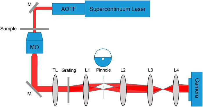
FIGURE 1. Setup scheme, containing an inverted microscope with a diffraction phase microscopy module positioned at its output. AOTF, acousto-optic tunable filter; M, mirror; sample; MO, microscope objective; TL, tube lens; L1-L4, lenses.

Phase Retrieval

Off-axis holography captures the complex wavefront of the sample by inducing a small angle between the sample and reference beams. The interference pattern recorded by the digital camera is defined as follow:

$I_{sensor}={\left|E_s\right|}^2 +{\left|E_r\right|}^2+2\left|E_s\right|\left|E_r\right|\cos \left(\phi \prime \right),(1)$

where $E_r$ represents the reference beam, $E_s$ represents the sample beam, and $\phi \prime$ is the phase difference between the beams. After subtracting the phase induced by the off-axis angle and the phase of the reference beam, we get $\phi$, the phase of the sample, which is proportional to the OPD of the sample, as following:

$\phi \left(x,y\right)=\frac{2\pi }{\lambda }OPD\left(x,y\right)=\frac{2\pi }{\lambda }\Delta n\left(x,y\right)d\left(x,y\right),(2)$

where λ is the illumination wavelength. The OPD value obtained at each point is equal to the product of the sample thickness $d\left(x,y\right)$ at that point and the integral refractive-index difference $\Delta n\left(x,y\right)$ at this point. $\Delta n\left(x,y\right)$ refers to the difference between the integral refractive index of the cell and the refractive index of the surrounding media, where the latter typically equals 1.33 for cells in a watery medium. After the acquisition of the off-axis hologram, we Fourier transform it. To cancel the effect of the off-axis angle, we filter out one of the cross-correlation terms, containing the complex wavefront of the sample [39]. An inverse Fourier transform of this cross-correlation term results in the complex wavefront of the sample, and its phase argument is the wrapped phase of the sample. Next, we apply a digital 2D phase unwrapping algorithm to avoid 2π ambiguities [40].

Spatial Fluctuation Analysis

We applied a spatial analysis on each of the quantitative phase maps of the cells, which represents the spatial fluctuation metric [35]. Phase variance, $\langle \Delta \phi {\left(x,y\right)}^2\rangle$ is calculated from the phase image in a window of 3 × 3 diffraction limited spots surrounding each pixel $\left(x,y\right)$, which is directly proportional to the variance of the refractive index difference, $\langle \Delta \phi {\left(x,y\right)}^2\rangle \propto \langle \Delta n{\left(x,y\right)}^2\rangle$. To calculate the phase spatial fluctuation metric, regardless of the sample thickness, the phase variance is normalized by the mean square phase in the corresponding 3 × 3 window of diffraction limited spots, $\overline{{\phi }^2}\left(x,y\right)$, to create the phase fluctuation map, $\langle \text{Δ}\phi ={\left(x,y\right)}^2\rangle /\overline{{\phi }^2}\left(x,y\right)$. By multiplying by the illumination wavelength and dividing by 2π, the OPD fluctuation map is obtained. In the following analysis, we emitted the cell edges, which are expected to have a significantly higher fluctuation amplitude and thresholded out noisy points. Finally, all the values were normalized. Figure 2 presents an OPD map of one of the SW620 cells analyzed and the resulting spatial fluctuation map. To ensure that the spatial fluctuations are not absorbed inside noise level, we calculate the system sensitivity by measuring the spatial standard deviation of the OPD profile of 3.254 nm, and temporal standard deviation of 0.282 nm.

FIGURE 2

FIGURE 2. (A) OPD image of an SW620 cell. (B) The resulting spatial fluctuation map. The OPD fluctuation at each point is calculated by the OPD variance divided by the mean squared OPD of a window of 3 × 3 of diffraction-limited spots [35]. The examined area, excluding the cell edges, is marked with a dashed black line.

Classification

We used Bottleneck Features network for binary classification in Keras. We trained a VGG16 structure network. This network has been previously proven as an effective feature-extraction classification network [41], and reached a rapid convergence on the given dataset. We attunemented the fully connected layers for binary classification between primary cancer cells and metastatic cancer cells, both isolated from the same individual. The network architecture is shown in Figure 3. We used 830 images for each class, obtained after 5× augmentation of the acquired data, rotations of 90, 180, and 270°, and an additional frame acquired at an additional time point after a second. The augmented data was divided 80, 10, and 10% into training, testing, and validation sets, respectively. To check independence in this selection, this division was done 5 times randomly, followed by new training, testing, and validation processes. Each time, we trained the network from scratch to ensure a stable division between the groups and that the network maintained a similar accuracy average. We trained the same network structure for each of the two classifiers. We then compared the results of the network for classification done separately based on the direct phase analysis and the spatial fluctuation analysis. The weights were frozen after 40 epochs, and the batch size was 10. The optimal selection of the hyperparameters was done after achieving convergence in the shortest time without causing overfitting. As verified, changing the hyperparameters did not result in better performance. The network converged after a few seconds when running on Google Colab GPU. Figure 4 presents the holograms, the quantitative phase maps, and the spatial fluctuation maps for each cell type, where the two latter ones are separately used as the inputs to the two networks. As can be seen when comparing Figures 4C,F one of the most prominent distinctions between the SW480 and SW620 cells is more ‘hot’ areas in the SW620 cell appearing after the spatial analysis.

FIGURE 3

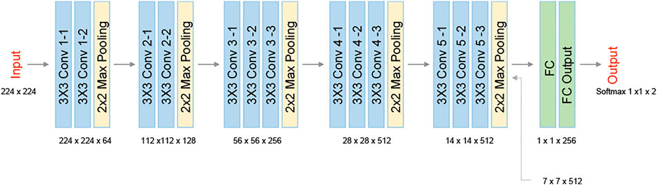
FIGURE 3. VGG16 network architecture. The network contains five 2-D convolutional layers, two fully connected layers (FC), and two classes at the output.

FIGURE 4

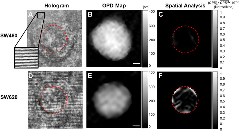
FIGURE 4. Examples of the databases, which were used for training the two deep neural networks. (A–C) SW480 primary cancer cell. (D–F) SW620 metastatic cancer cell. (A, D) Off-axis holograms. (B, E) Quantitative OPD maps. (C, F) The fluctuation maps obtained after the spatial analysis.

Results and Discussion

We examined the network performances on direct phase images and on the further-processed spatial analysis images. Figure 5 shows the accuracy and loss versus epochs for both the training and the validation stages for the two analyses. The overall deep-learning classification performance results are also summarized in Table 1. Here SW620 is defined as “positive” and SW480 as “negative”. The best result was observed for using the spatial analysis, with an accuracy of 92.5% and loss of 0.24. The direct phase analysis yielded a worse result, with an accuracy of 78.26% and loss of 0.45.

FIGURE 5

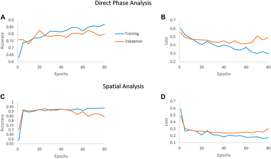
FIGURE 5. Accuracy and loss of the deep networks as they converge when classifying between the SW480 and SW620 cell lines. The blue line represents the training set, and the orange line represents the testing set. (A, B) The convergence of the direct phase analysis model. (C, D) The convergence of the spatial analysis model.

TABLE 1

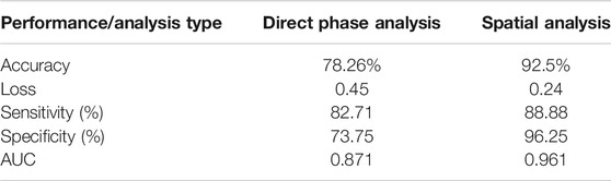
TABLE 1. Network performance results for each analysis.

As shown in Table 1, the spatially processed data yielded significantly higher accuracy, lower loss, higher sensitivity, higher specificity, and higher AUC, compared to those obtained when classifying the quantitative phase profiles directly. This validates the fact that the spatial analysis on the quantitative phase is beneficial as a preliminary step even for an automatic classifier that can theoretically find the best features for classification by itself.

In comparison, in Ref. [36] simple machine-learning classifier, based on a support vector machine and principal component analysis, was used on hand-crafted features extracted from the quantitative phase maps of the cell lines. This previous study achieved limited results for classifying SW480 and SW620 cell lines based on the spatial morphological information. In this case, hidden features in the image might be missed. In principle, deep-learning techniques can better classify by finding the best features automatically as the network is trained. However, they require a large number of examples with known classes in the training set. In our case, we had only 133 images, 5× augmented, from each cell type in the training set, which resulted in low performances (78.26% accuracy) when applying the network directly on the quantitative phase profiles. The TOP-GAN technique [37] is one of the techniques that can cope with the problem of a small training set, provided that unclassified examples (e.g., unclassified quantitative phase maps of other cell types) are available. This requires efforts of acquiring and processing many quantitative phase maps of another cell type. Here, we use another approach to cope with the small training set problem, first decreasing the differences between the quantitative phase maps of the two groups that do not contribute to the classification itself. Thus, we focused on classification based on the cell spatial flucuations, rather than the cell morphology, providing us good classification results even though a small training set is available.

In general, it was previously shown that pre-preprocessing on the data such as centering, scaling, and decorrelating known as data whitening [42], and spatial transformation [43] can help in speeding the training, reducing nuisances and redundancies, and improving the classification performance [44]. Thus, the preprocessing manipulation step standardizes and improves the dataset quality for the subsequent deep neural-network training.

In this paper, the chosen preprocessing is the spatial analysis that extracts the fluctuation map from quantitative phase images. As shown in Table 1, this indeed resulted in better accuracy (92.5% instead of 78.26%), better sensitivity (88.88% instead 82.71%), and better specificity (96.25% instead of 73.75%) compared to the direct phase analysis.

Conclusion

We presented an automatic deep-learning approach for the classification of live cancer cells by interferometric phase microscopy without staining. We examined two analyses, for which the resulting images are used as the inputs to the deep-learning network. The goal was classification between a pair of two types of live cells that were originated from the same organ of the same donor, SW480 cells, colorectal adenocarcinoma cells from colon tissue, and SW620 cells, metastatic cells from a lymph node from colon tissue. The first deep-learning classifier worked on the quantitative phase maps of the cell directly, and the second one used spatial analysis, which produced cell phase fluctuation maps representing the variance of the refractive-index difference. 332 off-axis holograms were acquired, 166 from each cell type, with 133 images from each cell type in the training set. This is considered a small training set for deep learning. For network training, data augmentation was applied to enlarge our dataset to a total number of 665 images for each class. We trained the same VGG16 neural network structure with the same number of epochs on each of the analyses. The pre-processed phase profiles yielding the spatial fluctuation maps resulted in significantly better results with the highest accuracy (92.5%) and the lowest loss. On the other hand, the direct phase analysis presented worse results, with an accuracy of 78.26% and higher loss. This demonstrates that the use of the phase fluctuation maps resulted from the spatial transformation analysis, before inputting them to the network, reduces nuisances and make the input less redundant, aiding to obtain better classification results in case of using a small training set in deep learning. The present study is expected to bring to an automatic, non-subjective cancer-cell classification, correlating the cancer-cell refractive-index distribution, as measured by stain-free interferometric phase imaging, and the cell metastatic potential.

Data Availability Statement

The raw data supporting the conclusion of this article will be made available by the authors, without undue reservation.

Author Contributions

NR-N designed and built the setup, conducted experiments, designed and implemented the algorithms, processed the data, and wrote the paper. NTS, conceived the idea, designed the setup, and algorithms, wrote the paper, and supervised the project.

Funding

H2020 European Research Council (ERC) (678316).

Conflict of Interest

The authors declare that the research was conducted in the absence of any commercial or financial relationships that could be construed as a potential conflict of interest.

Publisher’s Note

All claims expressed in this article are solely those of the authors and do not necessarily represent those of their affiliated organizations, or those of the publisher, the editors and the reviewers. Any product that may be evaluated in this article, or claim that may be made by its manufacturer, is not guaranteed or endorsed by the publisher.

Acknowledgments

We thank Dr. Raja Giryes from Tel Aviv University for useful discussions.

References

1. Armakolas A, Panteleakou Z, Nezos A, Tsouma A, Skondra M, Lembessis P, et al. Detection of the Circulating Tumor Cells in Cancer Patients. Future Oncol (2010) 6:1849–56. doi:10.2217/fon.10.152

PubMed Abstract | CrossRef Full Text | Google Scholar

2. Danova M, Torchio M, Mazzini G. Isolation of Rare Circulating Tumor Cells in Cancer Patients: Technical Aspects and Clinical Implications. Expert Rev Mol Diagn (2011) 11:473–85. doi:10.1586/erm.11.33

PubMed Abstract | CrossRef Full Text | Google Scholar

3. Kim SI, Jung H-i. Circulating Tumor Cells: Detection Methods and Potential Clinical Application in Breast Cancer. J Breast Cancer (2010) 13:125–31. doi:10.4048/jbc.2010.13.2.125

CrossRef Full Text | Google Scholar

4. Yu M, Stott S, Toner M, Maheswaran S, Haber DA. Circulating Tumor Cells: Approaches to Isolation and Characterization. J Cell Biol. (2011) 192:373–82. doi:10.1083/jcb.201010021

CrossRef Full Text | Google Scholar

5. Zieglschmid V, Hollmann C, Böcher O. Detection of Disseminated Tumor Cells in Peripheral Blood. Crit Rev Clin Lab Sci (2005) 42:155–96. doi:10.1080/10408360590913696

PubMed Abstract | CrossRef Full Text | Google Scholar

6. Farrell J. Abstract: The Origin of Cancer and the Role of Nutrient Supply: a New Perspective. Med Hypotheses (1988) 25:119–23. doi:10.1016/0306-9877(88)90029-1

PubMed Abstract | CrossRef Full Text | Google Scholar

7. Suresh S. Biomechanics and Biophysics of Cancer Cells. Acta Biomater (2007) 3:413–38. doi:10.1016/j.actbio.2007.04.002

PubMed Abstract | CrossRef Full Text | Google Scholar

8. Cross SE, Jin Y-S, Rao J, Gimzewski JK. Nanomechanical Analysis of Cells from Cancer Patients. Nat Nanotech (2007) 2:780–3. doi:10.1038/nnano.2007.388

CrossRef Full Text | Google Scholar

9. Cross SE, Jin Y-S, Tondre J, Wong R, Rao J, Gimzewski JK. AFM-based Analysis of Human Metastatic Cancer Cells. Nanotechnology (2008) 19:384003. doi:10.1088/0957-4484/19/38/384003

PubMed Abstract | CrossRef Full Text | Google Scholar

10. Singh R, Kumar S, Liu F-Z, Shuang C, Zhang CB, Jha R, et al. Etched Multicore Fiber Sensor Using Copper Oxide and Gold Nanoparticles Decorated Graphene Oxide Structure for Cancer Cells Detection. Biosens Bioelectron (2020) 168:112557. ‏doi:10.1016/j.bios.2020.112557

PubMed Abstract | CrossRef Full Text | Google Scholar

11. Guo X, Bonin K, Scarpinato K, Guthold M. The Effect of Neighboring Cells on the Stiffness of Cancerous and Non-cancerous Human Mammary Epithelial Cells. New J Phys (2014) 16:105002.

CrossRef Full Text | Google Scholar

12. Rother J, Nöding H, Mey I, Janshoff A. Atomic Force Microscopy-Based Microrheology Reveals Significant Differences in the Viscoelastic Response between Malign and Benign Cell Lines. Open Biol (2014) 4:140046. doi:10.1098/rsob.140046

PubMed Abstract | CrossRef Full Text | Google Scholar

13. Ahmmed SM, Bithi SS, Pore AA, Mubtasim N, Schuster C, Gollahon LS, et al. Multi-sample Deformability Cytometry of Cancer Cells. APL Bioeng (2018) 2:032002. doi:10.1063/1.5020992

PubMed Abstract | CrossRef Full Text | Google Scholar

14. Swaminathan V, Mythreye K, O'Brien ET, Berchuck A, Blobe GC, Superfine R. Mechanical Stiffness Grades Metastatic Potential in Patient Tumor Cells and in Cancer Cell Lines. Cancer Res (2011) 71:5075–80. doi:10.1158/0008-547210.1158/0008-5472.CAN-11-0247

PubMed Abstract | CrossRef Full Text | Google Scholar

15. Bhadriraju K, Hansen LK. Extracellular Matrix- and Cytoskeleton-dependent Changes in Cell Shape and Stiffness. Exp Cell Res (2002) 278:92–100. doi:10.1006/excr.2002.5557

PubMed Abstract | CrossRef Full Text | Google Scholar

16. Bao G, Suresh S. Cell and Molecular Mechanics of Biological Materials. Nat Mater (2003) 2:715–25. doi:10.1038/nmat1001

PubMed Abstract | CrossRef Full Text | Google Scholar

17. Yamaguchi H, Condeelis J. Regulation of the Actin Cytoskeleton in Cancer Cell Migration and Invasion. Biochim Biophys Acta (Bba) - Mol Cell Res (2007) 1773:642–52. doi:10.1016/j.bbamcr.2006.07.001

CrossRef Full Text | Google Scholar

18. Fife CM, McCarroll JA, Kavallaris M. Movers and Shakers: Cell Cytoskeleton in Cancer Metastasis. Br J Pharmacol (2014) 171:5507–23. doi:10.1111/bph.12704

CrossRef Full Text | Google Scholar

19. Alcaraz J, Buscemi L, Grabulosa M, Trepat X, Fabry B, Farré R, et al. Microrheology of Human Lung Epithelial Cells Measured by Atomic Force Microscopy. Biophysical J (2003) 84(3):2071–9. doi:10.1016/S0006-3495(03)75014-0

CrossRef Full Text | Google Scholar

20. Puig-de-Morales-Marinkovic M, Turner KT, Butler JP, Fredberg JJ, Suresh S. Viscoelasticity of the Human Red Blood Cell. Am J Physiology-Cell Physiol (2007) 293(2):C597–C605. doi:10.1152/ajpcell.00562.2006

CrossRef Full Text | Google Scholar

21. Svoboda K, Block SM. Biological Applications of Optical Forces. Annu Rev Biophys Biomol Struct (1994) 23:247–85. doi:10.1146/annurev.bb.23.060194.001335

PubMed Abstract | CrossRef Full Text | Google Scholar

22. Engström KG, Möller B, Meiselman HJ. Optical Evaluation of Red Blood Cell Geometry Using Micropipette Aspiration. Blood Cells (1992) 18(2241–257):241–65.

PubMed Abstract | Google Scholar

23. Guck J, Schinkinger S, Lincoln B, Wottawah F, Ebert S, Romeyke M, et al. Optical Deformability as an Inherent Cell Marker for Testing Malignant Transformation and Metastatic Competence. Biophysical J (2005) 88:3689–98. doi:10.1529/biophysj.104.045476

CrossRef Full Text | Google Scholar

24. Beil M, Micoulet A, von Wichert G, Paschke S, Walther P, Omary MB, et al. Sphingosylphosphorylcholine Regulates Keratin Network Architecture and Visco-Elastic Properties of Human Cancer Cells. Nat Cell Biol (2003) 5:803–11. doi:10.1038/ncb1037

PubMed Abstract | CrossRef Full Text | Google Scholar

25. Suresh S, Spatz J, Mills JP, Micoulet A, Dao M, Lim CT, et al. Connections between Single-Cell Biomechanics and Human Disease States: Gastrointestinal Cancer and Malaria. Acta Biomater (2005) 1:15–30. doi:10.1016/j.actbio.2004.09.001

PubMed Abstract | CrossRef Full Text | Google Scholar

26. Girshovitz P, Shaked NT. Generalized Cell Morphological Parameters Based on Interferometric Phase Microscopy and Their Application to Cell Life Cycle Characterization. Biomed Opt Express (2012) 3(8):1757–73. doi:10.1364/BOE.3.001757

PubMed Abstract | CrossRef Full Text | Google Scholar

27. Shaked NT. Quantitative Phase Microscopy of Biological Samples Using a Portable Interferometer. Opt Lett (2012) 37:2016–9. doi:10.1364/ol.37.002016

PubMed Abstract | CrossRef Full Text | Google Scholar

28. Girshovitz P, Shaked NT. Compact and Portable Low-Coherence Interferometer with off-axis Geometry for Quantitative Phase Microscopy and Nanoscopy. Opt Express (2013) 21:5701–14. doi:10.1364/oe.21.005701

PubMed Abstract | CrossRef Full Text | Google Scholar

29. Nativ A, Shaked NT. Compact Interferometric Module for Full-Field Interferometric Phase Microscopy with Low Spatial Coherence Illumination. Opt Lett (2017) 42:1492–5. doi:10.1364/ol.42.001492

PubMed Abstract | CrossRef Full Text | Google Scholar

30. Rotman-Nativ N, Turko NA, Shaked NT Flipping Interferometry with Doubled Imaging Area. Opt Lett (2018) 43(22):5543–5. doi:10.1364/OL.43.005543

PubMed Abstract | CrossRef Full Text | Google Scholar

31. Yaqoob Z, Yamauchi T, Choi W, Fu D, Dasari RR, Feld MS. Single-Shot Full-Field Reflection Phase Microscopy. Opt Express (2011) 19:7587–95. doi:10.1364/oe.19.007587

PubMed Abstract | CrossRef Full Text | Google Scholar

32. Javidi B, Markman A, Rawat S, O’Connor T, Anand A, Andemariam B. Sickle Cell Disease Diagnosis Based on Spatio-Temporal Cell Dynamics Analysis Using 3D Printed Shearing Digital Holographic Microscopy. Opt Express (2018) 26:13614–27. doi:10.1364/oe.26.013614

PubMed Abstract | CrossRef Full Text | Google Scholar

33. O’Connor T, Anand A, Andemariam B, Javidi B. Deep Learning-Based Cell Identification and Disease Diagnosis Using Spatio-Temporal Cellular Dynamics in Compact Digital Holographic Microscopy. Biomed Opt Express (2020) 11:4491–508. doi:10.1364/BOE.399020

PubMed Abstract | CrossRef Full Text | Google Scholar

34. Bishitz Y, Gabai H, Girshovitz P, Shaked NT. Optical-mechanical Signatures of Cancer Cells Based on Fluctuation Profiles Measured by Interferometry. J Biophoton (2014) 7(8):624–30. doi:10.1002/jbio.201300019

CrossRef Full Text | Google Scholar

35. Eldridge WJ, Steelman ZA, Loomis B, Wax A. Optical Phase Measurements of Disorder Strength Link Microstructure to Cell Stiffness. Biophysical J (2017) 112(4):692–702. doi:10.1016/j.bpj.2016.12.016

PubMed Abstract | CrossRef Full Text | Google Scholar

36. Roitshtain D, Wolbromsky L, Bal E, Greenspan H, Satterwhite LL, Shaked NT. Quantitative Phase Microscopy Spatial Signatures of Cancer Cells. Cytometry A (2017) 91(5):482–93. doi:10.1002/cyto.a.23100

PubMed Abstract | CrossRef Full Text | Google Scholar

37. Rubin M, Stein O, Turko NA, Nygate Y, Roitshtain D, Karako L, et al. TOP-GAN: Stain-free Cancer Cell Classification Using Deep Learning with a Small Training Set. Med Image Analmedical Image Anal (2019) 57:176–85. doi:10.1016/j.media.2019.06.014

PubMed Abstract | CrossRef Full Text | Google Scholar

38. Bhaduri B, Pham H, Mir M, Popescu G. Diffraction Phase Microscopy with White Light. Opt Lett. (2012) 37(6):1094–6. doi:10.1364/OL.37.001094

PubMed Abstract | CrossRef Full Text | Google Scholar

39. Girshovitz P, Shaked NT. Fast Phase Processing in off-axis Holography Using Multiplexing with Complex Encoding and Live-Cell Fluctuation Map Calculation in Real-Time. Opt Express (2015) 23:8773–87. doi:10.1364/oe.23.008773

PubMed Abstract | CrossRef Full Text | Google Scholar

40. Ghiglia DC, Pritt MD. Two-Dimensional Phase Unwrapping Theory, Algorithms, and Software. New York: John Wiley & Sons (1998).

Google Scholar

41. Simonyan K, Zisserman A. Very Deep Convolutional Networks for Large-Scale Image Recognition. NY, US: arXiv(2014). p. 1409–556.

Google Scholar

42. LeCun Y, Bottou L, Orr GB, Müller K-R. Neural Networks: Tricks of the Trade. LNCS (1998) 7700:9–50. doi:10.1007/3-540-49430-8_2

CrossRef Full Text | Google Scholar

43. Jaderberg M, Simonyan K, Zissermanm A, Kavukcuoglu K. Spatial Transformer Networks. Proceedings of the 28th International Conference on Neural Information Processing Systems; 2015 Dec 7-12; Montreal, Canada. NIPS (2015).

Google Scholar

44. Uka A, Polisi X, Barthes J, Halili AN, Skuka F, Vrana NE. Effect of Preprocessing on Performance of Neural Networks for Microscopy Image Classification. 2020 International Conference on Computing, Electronics & Communications Engineering (iCCECE); 2020 Aug 17-18; Southend, UK (2020) 162–5. doi:10.1109/iCCECE49321.2020.9231071

CrossRef Full Text | Google Scholar