 Wenbo Song
 Wei Sheng
 Dong Li
 Chong Wu2
- 1School of Mechanical, Electrical and Information Engineering, Shandong University, Weihai, China
- 2School of Management, Harbin Institute of Technology, Harbin, China
- 3School of Computer Science and Technology, Shandong University, Qingdao, China
The network topology of complex networks evolves dynamically with time. How to model the internal mechanism driving the dynamic change of network structure is the key problem in the field of complex networks. The models represented by WS, NW, BA usually assume that the evolution of network structure is driven by nodes’ passive behaviors based on some restrictive rules. However, in fact, network nodes are intelligent individuals, which actively update their relations based on experience and environment. To overcome this limitation, we attempt to construct a network model based on deep reinforcement learning, named as NMDRL. In the new model, each node in complex networks is regarded as an intelligent agent, which reacts with the agents around it for refreshing its relationships at every moment. Extensive experiments show that our model not only can generate networks owing the properties of scale-free and small-world, but also reveal how community structures emerge and evolve. The proposed NMDRL model is helpful to study propagation, game, and cooperation behaviors in networks.
1 Introduction
There are many complex systems in nature and human society, and most of which can be abstractly modeled as complex networks composed of nodes and links between nodes. The common social network, internet network, urban transportation network and gene regulatory network are typical complex networks. The rise of complex network theory provides a new perspective for the research of complex system science, and is of great significance to understanding the natural phenomena and the law of social operation.
Complex networks are dynamic systems that change continuously with time. How to construct network evolution models is the core problem of the complex network research. On the one hand, the network model helps to reveal the internal mechanism driving the dynamic evolution of network topology. On the other hand, as the network structure supports the physical behavior on the network, the network model also plays an important role in the study of network behaviors. Therefore, the network model is the basis of understanding network structure and function, their related studies have been widely applied in social computing [1], information retrieval, intelligent transportation, bioinformatics and other fields.
The studies of network evolution models started from 1959, the classical random network model was developed by Erdos and Renyi [2], named as ER model. This model assumes that links between nodes are generated with a random probability. With the development of data processing technology, researchers found that many real complex networks are not random networks. Aiming at this limitation, Watts et al. [3], Newman et al. [4] and Kleinberg [5] proposed small world models, which are able to explain some structure characteristics (i.e., short average distance and large clustering coefficient) of real complex networks. At the same time, the scale-free network models were developed, which leverage the mechanism of preferential connection, redirection or copy to interpret the power-law property of the node degree distribution. In recent years, following the above typical models, new mechanisms represented by weight [6–9], local world [10, 11], nonlinear growth [11–14], location information [15–18], popularity and homophily [19–21], and triangle closure [22–26] are used to construct network evolution models.
The construction idea of the existing network models are as following: based on data analysis and experimental observation, the corresponding increase and decrease rules of nodes and relationships are formulated, and nodes passively perform edge deletion and addition behaviors according to these rules. Although the existing models can generate networks that meet some characteristics of real networks, they all ignore the fact that each node in the network is an autonomous intelligent individual, and it should actively update its social relations based on their own experience and surrounding environment. The autonomous behavior of each node eventually leads to the dynamic evolution of the whole network.
Deep reinforcement learning is a subject of decision optimization, and the dynamic evolution of network is the results of node decisions. Based on the above facts, leveraging deep reinforcement learning to build a network model should be a meaningful attempt. In this paper, we propose a network modeling method based on deep reinforcement learning called the NMDRL model. In the NMDRL model, each node in the network is regarded as an agent, which continuously gains experience by taking actions to change its current state and obtaining corresponding rewards. At the same time, the agent learns to optimize its own action selection strategy by using a large amount of experience to make its autonomous decision more intelligent. After a large number of experiments, it has been shown that the NMDRL model evolves to generate a network that conforms well to the power-law distribution and the small-world characteristics of the real network. In addition, the model reproduces the emergence, growth, fusion, split and disappear of community in the evolutionary network.
The remainder of this article is structured in the following manner. In section 2, we detail the process of our model building, and a more detailed training process of the NMDRL model algorithm is included. The results of our experiments are presented in section 3. Finally, in section 4 we present the conclusion and discussion.
2 Model
2.1 NMDRL Model Overview
Different from existing network models simulating the network dynamic process under some rules, we propose the deep reinforcement learning-based model without any limitation rule, referred to as NMDRL model. As the network topology structure data suffers from high dimensionality and low efficiency, our NMDRL model is developed in a low-dimensional latent space in which each node is represented as a vector. At the same time, we also construct the transforming mechanism between network low-dimensional vector representation and high dimensional topology representation.
In the NMDRL model, the dynamic evolution process of complex network is modeled as a Markovian decision process, and each network node is considered as an intelligent agent. Every agent interacts with the environment and accumulates experience through continuous exploration attempts. At the same time, the agent also can use the accumulated experience to update its parameters, enhance its intelligence and help itself to make better autonomous decisions. Following deep reinforcement learning, each agent in our model owns four basic attributes:
• States: S represents all the states in the environment, and the agent can make certain responses by sensing the states of the environment. In the NMDRL model, a two-dimensional space is decomposed into some grids with the same size, and each grid is resumed as a state. We can change the number of states by adjusting parameters (i.e., row number and column number).
• Actions: A represents all the actions of the agent. In the low-dimensional space, the agent has six actions in total: up, down, left, right, stay and random. “stay” means the agent does not move its position, and “random” means that the agent randomly selects one from all states.
• Reward: R represents the reward or penalty of an agent after taking an action. The reward is returned from the environment use to evaluate the action performed by an agent. When an agent moves from one state to another state, the reward obtained by this agent is the number of all nodes located in the new state. For example, an agent i moves from state 1 to state 2, and there are 10 agents in the state 2. In this situation, the reward obtained by agent i is 10.
• Policy: Q is the behavior function of an agent. It determines how the agent chooses its next action. In this paper, the Q function is fitted by a neural network with the parameters Θ. There are two popular strategies for action selection through the behavior function. 1) The action corresponding to the biggest value of Q can be chosen, this strategy is called the greedy policy. 2) The ϵ-greedy policy, which is a strategy including both random and greedy policies. The formula of the ϵ-greedy policy is as following:
In order to ensure that the agent continues to explore the environment and fully make use of its existing experience, our NMDRL model adopts the ϵ-greedy policy.
2.2 NMDRL Model Training
In the NMDRL model, each node in the network is considered as an agent. This section introduces how to train the NMDRL model, and makes each agent have the ability to make autonomous decisions in the process of network evolution. As shown in Figure 1, the NMDRL model training mainly includes network evolution practice and agent strategy optimization.
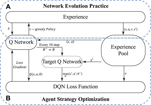
FIGURE 1. NMDRL training flow. (A) is the network evolution practice part of the algorithm, (B) is the agent strategy optimization part of the algorithm.
Specifically, Figure 1A shows the details of the network evolution practice, where the Q-network predicts the q-value of all the actions generated by the agent with state s, and then selects the action a according to the ϵ-greedy policy. Agent action will lead the network evolution. In this paper, the Q-network is implemented by a multilayer neural network presented in Figure 2. The neural network consists of an input layer, two hidden layers and an output layer, where the two hidden layers contain 128 and 64 neurons, respectively. The input of the neural network is the vector representation of the agent’s state, and the final output is the estimation Q of the agent action after the calculation of the two hidden layers. A quadruplet (s, a, r, s′) can be extracted from the above network evolution practice, and denoted as a piece of experience. The experience pool {(s1, a1, r1, s2)…(st, at, rt, st+1)… } is a collection of many experience data stored, and is used to train Q-network.
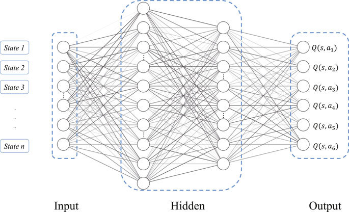
FIGURE 2. Structure of the NMDRL multilayer neural network.
In order to optimize the agent evolution strategy, we first need to define the loss function of the Q-network that is to minimize the reward error between the predicted and true values. According to the Bellman equation, the loss function of the Q-network is defined as given in Eq. 2, which ensures that the Q-network performs more effective learning.
The process of agent policy optimization part is shown in Figure 1B, where the agent will sample the experience randomly from the experience pool, put (s, a) into the Q-network to obtain the predicted Q value, use the maximum value obtained from s′ in the target Q-network as the target value. The parameters of the Q-network are updated using the loss function given in Eq. 2. At the same time, the target Q-network is updated once for every 10 updates to the Q-network. After continuously collecting and learning from the network evolution experience, the network evolution strategy of each agent is continuously updated. Finally, all the agents work together to model the network according to their own network evolution strategies.
Algorithm 1. Training Algorithm of the NMDRL.
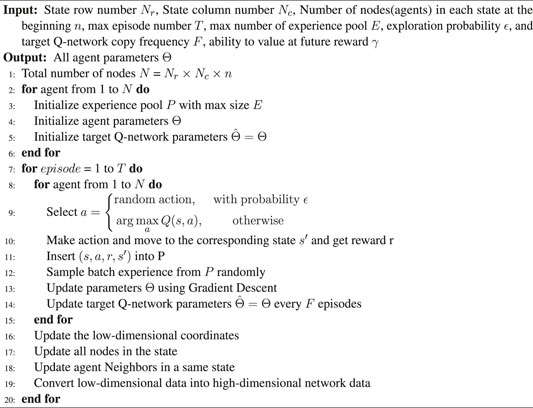
In summary, the detailed procedure of training the NMDRL network model is described in Algorithm 1. First, the experience pool, Q-network and target Q-network of all agents are initialized in lines 1–6. In lines 9–15, NMDRL training is performed for all agents, including the practice of network evolution and policy optimization. In lines 16–18, the global information obtained from the network evolution is updated. Finally, in line 19, the low-dimensional space data is transformed to the high-dimensional space data.
2.3 The Network Conversion Mechanism From Low-Dimension Representation to High-Dimension Representation
In the NMDRL model, the interactions among nodes and move behaviors of nodes are designed in a low-dimensional space. Therefore, a mechanism of converting a network from low-dimensional vector representation to high-dimensional topology representation is necessary.
The aids of the conversion mechanism are to add/delete edges and assign weights for these edges based on the network low-dimensional vector representation. In this paper, we make use of the threshold and attenuation rules to design this conversion mechanism. We assume that if two nodes are in a same state, an edge between them will be created. The weight of this edge will be weakened or enhanced over time. When the value of the weight is smaller than a threshold, this edge will be deleted. The details of the conversion mechanism are as following:
• If two nodes with no edge are in a same state, we create a new edge for these two nodes, and assign an initial weight winitial for this edge.
• If two nodes with an edge are not in a same state any more, the weight of the edge will be weaken. We denote the weight of the existing edge as wlast at the last time step. The new weight wcurrent at current time step is wlast/a, where a is the attenuation index. If two nodes owing one edge are not in a same state for several time steps, the edge weight will be continuously weakened. Once the new weight wcurrent is smaller than the threshold t, we believe that the relationship strength between the two nodes is too weak and this edge should no longer exist. This edge will be deleted.
• If two nodes with an edge are in a same state again, the weight of the edge will be strengthened. The new weight wcurrent at current time step is wlast/a+ winitial, where the former part is the attenuation of time to the past weight, and the second part is the enhancement of the weight when two nodes are in a same state.
3 Results
In this section, we conduct comprehensive experiments to validate the effectiveness of the NMDRL model from the following aspects: node degree distribution, network clustering coefficient, network average distance, community formation and evolution. In the experiments, we set row number and column number of two-dimensional space to be 10, so there are 100 states in total.
3.1 Degree Distribution
In a network, the degree of a node is the number of connections this node owns. The degree distribution P(k) of a network is defined to be the fraction of nodes in the network with degree k [27], which is an important index in studying complex networks. Here, we try to analyze the degree distributions of the networks generated by the NMDRL model.
Figure 3A shows the degree distributions of the networks generated by the NMDRL model, where orange, blue and green curves represent three networks containing 300, 500 and 700 nodes respectively. Other parameters γ and ϵ are set to be 0.8 and 0.6 respectively. It can be seen from Figure 3A that there are a small number of nodes with high degree and a large number of nodes with a low degree in the generated networks. This means that the degree distribution of the networks created by the NMDRL model follows the power-law distribution property. The exponent of the power-law distribution is between (2, 3), and the generated networks are scale-free networks.
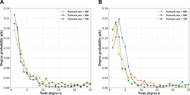
FIGURE 3. (A,B) are the degree distributions of the networks generated by NMDRL model.
Although power-law distribution is the most common degree distribution, not all real networks own this kind of degree distribution. Researchers find that some real networks obey the subnormal distribution which is between the normal distribution and the power-law distribution [28]. Here, we adjust the parameter ϵ from 0.6 to 0.7, and other parameters remain unchanged. Figure 3B presents the degree distributions of the generated networks with three sizes. We can see that the degree distributions of these networks follow the subnormal distribution form. All of the above results indicate that our NMDRL model is able to generate networks with power-law or subnormal distribution that exist in real networks.
3.2 Clustering Coefficient and Average Path Length
Clustering coefficient and average path length are also two classic metrics of complex networks. For a network, if its clustering coefficient is large and average path length is small, this network can be called a small-world network. Here, we try to explore whether the networks generated by the NMDRL model own the small-world property.
Figure 4A plots the change of clustering coefficient over 200-time steps for three network sizes. x-axis represents the time step, and y-axis represents the network clustering coefficient. Orange, blue and green curves are corresponding to three networks owing 300, 500 and 700 nodes respectively. It can be seen from Figure 4A that the value of the clustering coefficient is small in the early stage of network evolution. This is because that each grid in the two-dimensional space owns the same number of nodes at the initial time, therefore the initial network is a regular network in fact whose clustering coefficient is small. The clustering coefficient of the dynamic network increases from time 1 to 70, and changes a little from 71 to 200. This means that the dynamic network reaches the stable state with a high clustering coefficient.
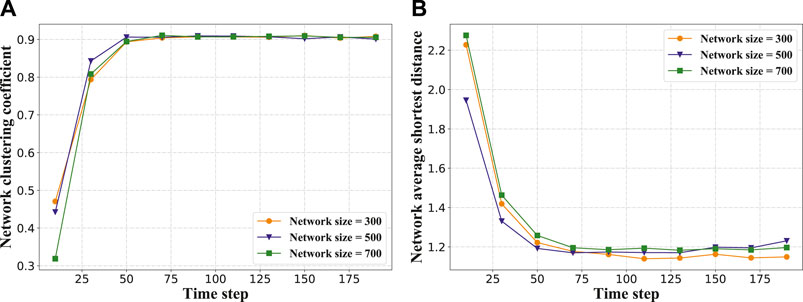
FIGURE 4. (A) is variation of network clustering coefficient with time step, (B) is variation of network average distance with time step.
Figure 4B plots the change of average path length over time for different network sizes. At the initial time step, the average path length of the network is relatively large. This value decreases from time 1 to 70, and changes a little from 71 to 200. The phenomenon observed from Figure 4A and Figure 4B indicates that our proposed model is able to drive a regular network to evolve into a network with a big clustering coefficient and small average path length (i.e., small-world network).
3.3 Community Emergence and Evolution
In this subsection, we try to analyze the community [29, 30] formation and evolution capability of the NMDRL model. Since our model is constructed in a low-dimensional space, and a network conversion mechanism from low-dimensional representation to high-dimensional representation is developed at the same time. This design makes us analyze and verify the model effect from both low and high dimensional levels.
Specifically, Figure 5 and Figure 6 show the network dynamic evolution process from time 1 to 200 in low-dimensional and high-dimensional spaces respectively. Both of these two figures clearly present the formation process of community structures in the network, and the communities in high and low dimensional spaces match each other very well. These observed results illustrate the effectiveness of our NMDRL model in terms of explaining the mechanism of community emergence on the one hand, and also support the rationality of our transformation mechanism on the other hand.
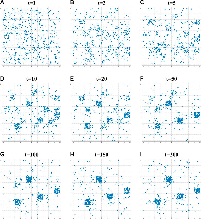
FIGURE 5. Demonstration of network evolution process in the low dimensional vector space with parameters γ = 0.2, ϵ = 0.2, network size = 500, (A) t = 1, (B) t = 3, (C) t = 5, (D) t = 10, (E) t = 20, (F) t = 50, (G) t = 100, (H) t = 150, (I) t = 200.
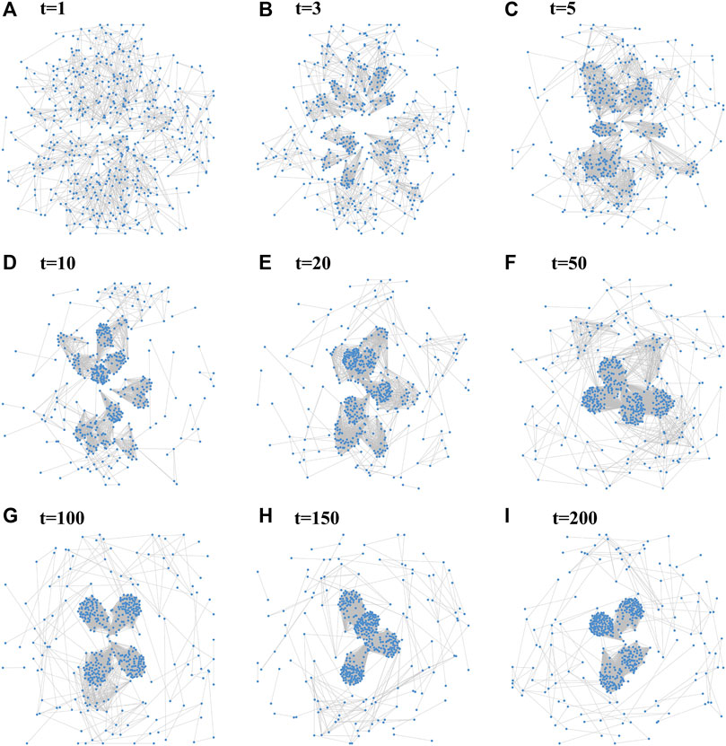
FIGURE 6. Demonstration of network evolution process in the high dimensional vector space with parameters γ = 0.2, ϵ = 0.2, network size = 500, (A) t = 1, (B) t = 3, (C) t = 5, (D) t = 10, (E) t = 20, (F) t = 50, (G) t = 100, (H) t = 150, (I) t = 200.
Besides community formation, we also find that our NMDRL model is able to reproduce several common evolutionary behaviors. 1) Growth. The size of the circular region in Figure 7A and Figure 7B shows a significant growth over time. 2) Fusion. Some smaller communities in Figure 7C move to the larger communities. They fuse together after some time steps and form some larger communities in Figure 7D. 3) Split. An extremely large community in Figure 7E splits into multiple smaller communities in Figure 7F. 4) Disappear. The community in the circular region in Figure 7G disappears in Figure 7H.
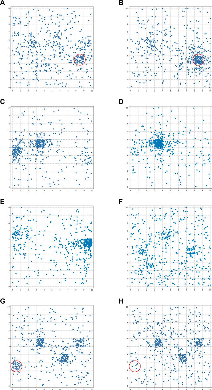
FIGURE 7. Evolutionary behaviors of communities. (A,B) presents community growth behavior, (C,D) presents community fusion behavior, (E,F) presents community split behavior, and (G,H) presents community disappear behavior.
In the NMDRL model, parameter ϵ is used to balance the ability of agent to explore and exploit. Here, we attempt to analyze the impact of ϵ on community emergence. Figure 8J presents the change of network modularity under different ϵ values. When ϵ is in the range of 0.1–0.5, network modularity is smoothly maintained at a high level. Start with ϵ = 0.5, network modularity sharply decreases and enters into a very low level. It is also observed that when ϵ > 0.7, the network will no longer have associations when the data in the low dimensional vector space shown in Figures 8A–I. This indicates that the ϵ is a key parameter of determining whether the community appears.
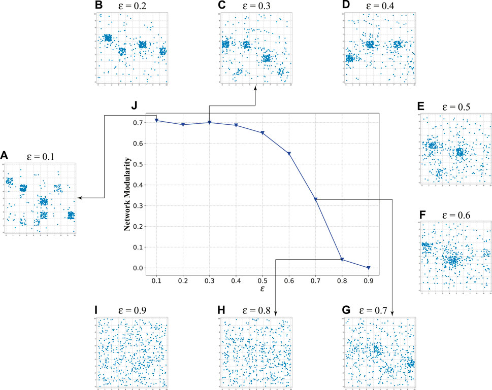
FIGURE 8. Impact of ϵ on the network community evolution process.(A–I) are the representations of ϵ in (0.1–0.9) in the low dimensional vector space, respectively, and (J) is the variation curve of network modularity with increasing ϵ.
4 Conclusion and Discussion
In view of the limitation of nodes passively updating relationships in the existing models, we try to leverage deep reinforcement learning to develop a network evolution model. In the model, each node considered as an agent interacts with its neighbors and makes strategic choices based on its utility at every moment. A large number of simulation results validate that the generated networks by our model have three most important structure characters of real networks: scale-free, small-world and community.
Some challenges remain. How to learn model parameters based on real networks and apply the learned model in some typical tasks (i.e. link prediction) is one of our future directions. To be more relevant, the impact of multiple agents with different intelligence on the evolving network will also be another direction of our future research.
Data Availability Statement
The original contributions presented in the study are included in the article/Supplementary Material, further inquiries can be directed to the corresponding author.
Author Contributions
WS: methodology, software, data analysis and writing-original draft. WS: data analysis, writing-review and editing. DL: conceptualization, methodology, writing–original draft and review. CW and JM: supervision, writing-review and editing.
Funding
This work is funded by the National Natural Science Foundation of China (Nos. 62076149, 61702138, 61602128, 61672322, 61672185, 72131005 and 71771066), and the Shandong Province Natural Science Foundation of China (No. ZR2016FQ13), and the China Postdoctoral Science Foundation (Nos. 2020T130368, 2019M662360, 2017M621275 and 2018T110301), and Young Scholars Program of Shandong University, China, Weihai (No. 1050501318006), and Science and Technology Development Plan of Weihai City, China (No. 1050413421912).
Conflict of Interest
The authors declare that the research was conducted in the absence of any commercial or financial relationships that could be construed as a potential conflict of interest.
Publisher’s Note
All claims expressed in this article are solely those of the authors and do not necessarily represent those of their affiliated organizations, or those of the publisher, the editors and the reviewers. Any product that may be evaluated in this article, or claim that may be made by its manufacturer, is not guaranteed or endorsed by the publisher.
References
1. Pei H, Yang B, Liu J, Chang K. Active Surveillance via Group Sparse Bayesian Learning. IEEE Trans Pattern Anal Mach Intell (2020) Online ahead of print. doi:10.1109/TPAMI.2020.3023092
2. Erdos P, Rényi A. On the Evolution of Random Graphs. Publ Math Inst Hung Acad Sci (1960) 5(1):17–60.
3. Watts DJ, Strogatz SH. Collective Dynamics of 'Small-World' Networks. Nature (1998) 393(6684):440–2. doi:10.1038/30918
4. Newman ME, Watts DJ. Renormalization Group Analysis of the Small-World Network Model. Phys Lett A (1999) 263(4-6):341–6. doi:10.1016/s0375-9601(99)00757-4
6. Yook SH, Jeong H, Barabási A-L, Tu Y. Weighted Evolving Networks. Phys Rev Lett (2001) 86(25):5835–8. doi:10.1103/physrevlett.86.5835
7. Zhou Y-B, Cai S-M, Wang W-X, Zhou P-L. Age-Based Model for Weighted Network with General Assortative Mixing. Physica A: Stat Mech its Appl (2009) 388(6):999–1006. doi:10.1016/j.physa.2008.11.042
8. Barrat A, Barthelemy M, Pastor-Satorras R, Vespignani A. The Architecture of Complex Weighted Networks. Proc Natl Acad Sci (2004) 101(11):3747–52. doi:10.1073/pnas.0400087101
9. Li P, Yu J, Liu J, Zhou D, Cao B. Generating Weighted Social Networks Using Multigraph. Physica A: Stat Mech its Appl (2020) 539:122894. doi:10.1016/j.physa.2019.122894
10. Li X, Chen G. A Local-World Evolving Network Model. Physica A: Stat Mech its Appl (2003) 328(1-2):274–86. doi:10.1016/s0378-4371(03)00604-6
11. Feng S, Xin M, Lv T, Hu B. A Novel Evolving Model of Urban Rail Transit Networks Based on the Local-World Theory. Physica A: Stat Mech its Appl (2019) 535:122227. doi:10.1016/j.physa.2019.122227
12. Feng M, Deng L, Kurths J. Evolving Networks Based on Birth and Death Process Regarding the Scale Stationarity. Chaos (2018) 28(8):083118. doi:10.1063/1.5038382
13. Liu J, Li J, Chen Y, Chen X, Zhou Z, Yang Z, et al. Modeling Complex Networks with Accelerating Growth and Aging Effect. Phys Lett A (2019) 383(13):1396–400. doi:10.1016/j.physleta.2019.02.004
14. Li J, Zhou S, Li X, Li X. An Insertion-Deletion-Compensation Model with Poisson Process for Scale-Free Networks. Future Generation Comput Syst (2018) 83:425–30. doi:10.1016/j.future.2017.04.011
15. Hristova D, Williams MJ, Musolesi M, Panzarasa P, Mascolo C. Measuring Urban Social Diversity Using Interconnected Geo-Social Networks. In: Proceedings of the 25th international conference on world wide web; 2016 May 11–15; Montreal, Canada (2016). p. 21–30. doi:10.1145/2872427.2883065
16. Noulas A, Shaw B, Lambiotte R, Mascolo C. Topological Properties and Temporal Dynamics of Place Networks in Urban Environments. In: Proceedings of the 24th International Conference on World Wide Web; 2015 May 18–22; Florence, Italy (2015). p. 431–41. doi:10.1145/2740908.2745402
17. Zhou L, Zhang Y, Pang J, Li C-T. Modeling City Locations as Complex Networks: An Initial Study. In: International Workshop on Complex Networks and their Applications; 2016 November 30–December 02; Milan, Italy. Springer (2016). p. 735–47. doi:10.1007/978-3-319-50901-3_58
18. Ding Y, Li X, Tian Y-C, Ledwich G, Mishra Y, Zhou C. Generating Scale-free Topology for Wireless Neighborhood Area Networks in Smart Grid. IEEE Trans Smart Grid (2018) 10(4):4245–52. doi:10.1109/TSG.2018.2854645
19. Muscoloni A, Cannistraci CV. A Nonuniform Popularity-Similarity Optimization (Npso) Model to Efficiently Generate Realistic Complex Networks with Communities. New J Phys (2018) 20(5):052002. doi:10.1088/1367-2630/aac06f
20. Papadopoulos F, Kitsak M, Serrano MÁ, Boguñá M, Krioukov D. Popularity versus Similarity in Growing Networks. Nature (2012) 489(7417):537–40. doi:10.1038/nature11459
21. Liu Y, Li L, Wang H, Sun C, Chen X, He J, et al. The Competition of Homophily and Popularity in Growing and Evolving Social Networks. Scientific Rep (2018) 8(1):1–15. doi:10.1038/s41598-018-33409-8
22. Holme P, Kim BJ. Growing Scale-free Networks with Tunable Clustering. Phys Rev E Stat Nonlin Soft Matter Phys (2002) 65(2):026107. doi:10.1103/PhysRevE.65.026107
23. Li G, Li B, Jiang Y, Jiao W, Lan H, Zhu C. A New Method for Automatically Modelling Brain Functional Networks. Biomed Signal Process Control (2018) 45:70–9. doi:10.1016/j.bspc.2018.05.024
24. Tang T, Hu G. An Evolving Network Model Based on a Triangular Connecting Mechanism for the Internet Topology. . In: International Conference on Artificial Intelligence and Security; 2019 July 26–28; New York, NY. Springer (2019). p. 510–9. doi:10.1007/978-3-030-24268-8_47
25. Overgoor J, Benson A, Ugander J. Choosing to Grow a Graph: Modeling Network Formation as Discrete Choice. In: The World Wide Web Conference; 2019 May 13–17; San Francisco, CA (2019). p. 1409–20.
26. Jia D, Yin B, Huang X, Ning Y, Christakis NA, Jia J. Association Analysis of Private Information in Distributed Social Networks Based on Big Data. Wireless Commun Mobile Comput (2021) 2021(1):1–12. doi:10.1155/2021/1181129
27. Barabási AL, Albert R. Emergence of Scaling in Random Networks. Science (1999) 286(5439):509–12. doi:10.1126/science.286.5439.509
28. Feng M, Qu H, Yi Z, Kurths J. Subnormal Distribution Derived from Evolving Networks with Variable Elements. IEEE Trans Cybern (2017) 48(9):2556–68. doi:10.1109/TCYB.2017.2751073
29. Zhang F, Liu H, Leung Y-W, Chu X, Jin B. Cbs: Community-Based Bus System as Routing Backbone for Vehicular Ad Hoc Networks. IEEE Trans Mobile Comput (2016) 16(8):2132–46. doi:10.1109/TMC.2016.2613869
Keywords: complex network, deep reinforcement learning, scale-free, small world, community evolution
Citation: Song W, Sheng W, Li D, Wu C and Ma J (2022) Modeling Complex Networks Based on Deep Reinforcement Learning. Front. Phys. 9:822581. doi: 10.3389/fphy.2021.822581
Received: 26 November 2021; Accepted: 22 December 2021;
Published: 14 January 2022.
Edited by:
Chao Gao, Southwest University, ChinaReviewed by:
Xin Sun, Harbin Institute of Technology, ChinaFusang Zhang, Institute of Software (CAS), China
Copyright © 2022 Song, Sheng, Li, Wu and Ma. This is an open-access article distributed under the terms of the Creative Commons Attribution License (CC BY). The use, distribution or reproduction in other forums is permitted, provided the original author(s) and the copyright owner(s) are credited and that the original publication in this journal is cited, in accordance with accepted academic practice. No use, distribution or reproduction is permitted which does not comply with these terms.
*Correspondence: Dong Li, ZG9uZ2xpQHNkdS5lZHUuY24=