Sensitivity analysis of the temperature profile changing law in the production string of a high-pressure high-temperature gas well considering the coupling relation among the gas flow friction, gas properties, temperature, and pressure

Introduction

Due to the worldwide rapid increase in the consumption and extensive application of natural gas for both industrial and civil purposes, natural gas development has stepped into more harsh strata and conditions, such as gas hydrate [1–3], shale/tight gas [4, 5], deep water formation [6, 7], deep/ultra-deep stratum [8, 9], and coalbed methane [10]. Among the aforesaid resources of natural gas, the deep/ultra-deep stratum has great potential for its rich reserves and high productivity. Deep/ultra-deep natural gas is usually buried 5,000 m or deeper under the ground, so the bottom hole temperature can be as high as 180 °C [11, 12]. As a result, the temperature profile in the production string is unavoidably changed by the natural gas from the reservoir. Meanwhile, the temperature profile is an important index for production safety. The applications are as follows. First is well integrity. The increase in temperature can lead to trapped annular pressure [13, 14]. This can cause casing collapse [15, 16], cement integrity failure [17, 18], packer sealing failure [19], and tubing deformation [20]. In addition to trapped annular pressure, thermal stress would also damage well integrity [21], such as the tubing buckling and cement strength reduction. Second is flow assurance. The wax and gas hydrate would block the production pathway when the temperature is not high enough [22, 23]. In some gas wells with high content of sulfur, sulfur deposition can also block the production pathway [24]. When the abovementioned incidents happen, effective measures such as heating, chemical plugging removal, and ultrasound removal [25, 26] must be taken to restart production. Third is the production test. The well temperature distribution can reflect the reservoir energy, so it is a classical method to estimate the productivity by analyzing the wellbore transient temperature during the production test [27, 28].

Henceforth, substantial efforts have been devoted to calculate the wellbore temperature. The available research works indicate that the calculation should consider different engineering conditions, such as cement hydration [29], drilling circulation [30], thermal insulation [31], and gas properties [32, 33]. For an HPHT gas well, there are two factors that cannot be ignored: first, the gas flow friction would generate heat and decrease pressure because of the high production rate [34]. Second, the gas properties would vary because the temperature and pressure decrease remarkably from the reservoir to the wellhead. For this reason, this study establishes a model to analyze the changing law of the temperature profile in HPHT gas wells. The model considers the gas flow friction and variation in properties in order to match the actual condition as closely as possible. A dimensionless index is introduced to evaluate the influencing factors, thus providing support for safe and effective production of HPHT gas wells.

Calculation method of the temperature profile inside the production string

Conservation law in the production string

The reservoir gas is the heat resource to redistribute the wellbore temperature. To calculate the temperature, some assumptions are essential. First, the wellbore cross-section is taken as a circle, and the pipes are concentric. Second, thermal conductivity is used to express the wellbore heat transfer capacity. Third, the production is stable without large fluctuations, and the heat transfer along the flow direction is so minor that it can be ignored. Based on the aforementioned assumptions, the energy conservation equation can be established in the micro-unit of the production string, including the internal energy, kinetic energy, pressure energy, gravitational potential energy, and heat transfer, as expressed by Eq. 1:

$C_{\mathrm{f}}\frac{\mathrm{d}{T}_{\mathrm{f}}}{\mathrm{d}z}+v_{\mathrm{f}}\frac{\mathrm{d}{v}_{\mathrm{f}}}{\mathrm{d}z}+\frac{1}{{\rho }_{\mathrm{f}}}\frac{\mathrm{d}p}{\mathrm{d}z}+g\sin \theta +\frac{1}{w_{\mathrm{f}}}\frac{\mathrm{d}Q}{\mathrm{d}z}=0(1)$

where C_f is the gas heat capacity inside the production string, J/(kgK); dT_f is the gas temperature change inside the production string, K; dz is the length of the micro-unit of the production string, m; v_f is the flow velocity of gas, m/s; dv_f is the flow velocity change of gas, m/s; ρ_f is the gas density inside the production string, kg/m³; p is the gas pressure inside the production string, Pa; g is the gravity speed, m/s²; θ is the well inclination angle, °; w_f is the gas mass flow rate, kg/s; and dQ is the heat transfer along the well radial direction, J/s.

In addition to the energy conservation law, the momentum conservation law can also be applied in the micro-unit of the production string, as expressed by Eq. 2:

$\frac{\mathrm{d}p}{\mathrm{d}z}+{\rho }_{\mathrm{f}}g\sin \theta +f\frac{{\rho }_{\mathrm{f}}{v}_{\mathrm{f}}^2}{2d_{\mathrm{t}\mathrm{n}}}+{\rho }_{\mathrm{f}}{v}_{\mathrm{f}}\frac{\mathrm{d}{v}_{\mathrm{f}}}{\mathrm{d}z}=0(2)$

where f is the friction efficient between the gas flow and production string, dimensionless; and d_tn is the inner diameter of the production string, m.

Likewise, the mass conservation law can also be applied in the micro-unit of the production string, as expressed by Eq. 3:

${\rho }_{\mathrm{f}}\frac{\mathrm{d}{v}_{\mathrm{f}}}{\mathrm{d}z}+v_{\mathrm{f}}\frac{\mathrm{d}{\rho }_{\mathrm{f}}}{\mathrm{d}z}=0.(3)$

Heat transfer along the well radial direction

The heat transfers through the tubing, annular liquid, casing, and cement sheath and finally comes to the formation. This process can be divided into two parts. The first part is the heat transfer from the production string to the cement sheath and the second is from the cement sheath to the formation. According to the semi-steady method [35, 36], the first part can be seen as a state, so the heat transfer can be expressed by Eq. 4:

$\mathrm{d}{Q_{\mathrm{r}}}_{\mathrm{w}}=\frac{T_{\mathrm{f}}-T_{\mathrm{h}}}{R_{\mathrm{t}\mathrm{o}}}\mathrm{d}z(4)$

where dQ_rw is the heat transfer from the production string to the cement sheath, J/s; T_f is the gas temperature inside the production string, K; T_h is the temperature of the cement sheath, K; and R_to is the thermal resistance from the production string to the cement sheath, mk/W.

As shown in Figure 1, R_to is the thermal resistance from the production string to the cement sheath and can be obtained by the thermal resistance series principle, as expressed by Eq. 5:

$R_{\mathrm{t}\mathrm{o}}=R_{\mathrm{t}\mathrm{c}\mathrm{t}}+R_{\mathrm{c}\mathrm{h}\mathrm{t}}+{\displaystyle \sum }_{k=1}^m{R}_{\mathrm{t}\mathrm{c}}^k+{\displaystyle \sum }_{j=1}^n{R}_{\mathrm{t}\mathrm{e}}^j(5)$

where R_tct is the thermal resistance of the tubing wall, mk/W; R_cht is the thermal resistance of the annular liquid, mk/W; R^k_tc is the thermal resistance of the kth casing wall, mk/W; and R^j_te is the thermal resistance of the jth cement sheath, mk/W.

FIGURE 1

FIGURE 1. Heat transfer along the well radial direction.

Hasan and Kabir [37] verified that the heat transfer from the cement sheath to the formation conforms to Fourier heat conduction law, which can be expressed by Eq. 6:

$\mathrm{d}{Q_{\mathrm{r}}}_{\mathrm{f}}=\frac{2\pi \lambda \mathrm{e}\left(T_{\mathrm{h}}-T_{\mathrm{e}}\right)}{T_{\mathrm{D}}}\mathrm{d}z(6)$

where λ_e is the formation of thermal conductivity outside the cement sheath, W/(mk); T_e is the temperature of the formation outside the cement sheath, k; and T_D is the dimensionless temperature of the formation outside the cement sheath, dimensionless.

The formation temperature can be expressed by Eq. 7 when the formation temperature is seen as a linear distribution:

$T_{\mathrm{e}}=T_{\mathrm{o}}+g_{\mathrm{t}}\left(h-z\right)(7)$

where T_o is the surface ground temperature, k; g_t is the geothermal gradient, k/100 m; h is the well depth, m; and z is the distance from the formation outside the cement sheath to the well bottom, m.

The dimensionless temperature of formation can be expressed by Eqs 8 and 9, as proposed by Hasan and Kabir [37]:

$T_D=\{\begin{array}{cc}1.1281\sqrt{t_D}\left(1-0.3\sqrt{t_D}\right),& t_D\le 1.5,\\ \left(0.4063+0.5\ln t_D\right)\left(1+0.6/t_D\right),& t_D\succ 1.5\end{array}(8)$

$tD=\frac{t\alpha \mathrm{e}}{r{\mathrm{w}}^2}(9)$

where t_D is the dimensionless production time, dimensionless; t is the production time, s; α_e is the formation thermal diffusion coefficient, m²/s; and r_w is the wellbore radius, m.

According to the semi-steady method and the conservation principle of radial heat flow, the heat transfer in the two aforementioned parts is equal. Then, the temperature of the cement sheath, T_h, can be expressed by Eq. 10:

$T_{\mathrm{h}}=\frac{T_{\mathrm{D}}{T}_{\mathrm{f}}+2\pi {\lambda }_{\mathrm{e}}{R}_{\mathrm{t}\mathrm{o}}{T}_{\mathrm{e}}}{T_{\mathrm{D}}+2\pi {\lambda }_{\mathrm{e}}{R}_{\mathrm{t}\mathrm{o}}}.(10)$

The heat transfer on the radial direction can be obtained by combining Eq. 10 and Eq. 6, as expressed by Eq. 11:

$\mathrm{d}\mathrm{Q}=\frac{2\pi {\lambda }_{\mathrm{e}}\left(T_{\mathrm{f}}-T_{\mathrm{e}}\right)}{T_{\mathrm{D}}+2\pi {\lambda }_{\mathrm{e}}{R}_{\mathrm{t}\mathrm{o}}}\mathrm{d}z.(11)$

Impact of the gas flow friction

The gas flow friction can increase the gas internal energy while decreasing the pressure energy. The friction efficient is the key parameter to calculate gas flow friction [38], as expressed by Eq. 12:

$f=\{\begin{array}{cc}\frac{64}{\mathrm{R}\mathrm{e}},& \mathrm{R}\mathrm{e}\le 2000\\ {\left[1.14-21g\left(\frac{R\mathrm{a}}{d_{\mathrm{t}\mathrm{n}}}+\frac{21.25}{{\mathrm{R}\mathrm{e}}^{0.9}}\right)\right]}^{-2},& \mathrm{R}\mathrm{e}>2000\end{array}(12)$

where R_a is the roughness of the production string inner wall, m; and Re is the Reynolds number, dimensionless.

The Reynolds number can be expressed by Eq. 13:

$\mathrm{R}\mathrm{e}=\frac{{\rho }_{\mathrm{f}}{v}_{\mathrm{f}}{d}_{\mathrm{t}\mathrm{n}}}{\mu }(13)$

where μ is the gas viscosity, Pas.

After the friction efficient is obtained, the gas pressure inside the production string can be expressed by Eq. 14:

$\frac{\mathrm{d}p}{\mathrm{d}z}=-{\rho }_{\mathrm{f}}g\sin \theta -f\frac{{\rho }_{\mathrm{f}}{v}_{\mathrm{f}}^2}{2d_{\mathrm{t}\mathrm{n}}}-{\rho }_{\mathrm{f}}{v}_{\mathrm{f}}\frac{\mathrm{d}{v}_{\mathrm{f}}}{\mathrm{d}z}(14)$

Likewise, the gas temperature in the production string can be obtained by substituting Eq. 15 and Eq. 11 into Eq. 1, as expressed by Eq. 14:

$\frac{\mathrm{d}{\mathit{T}}_{\mathrm{f}}}{\mathrm{d}\mathit{z}}=\mathit{f}\frac{{\rho }_{\mathrm{f}}{\mathrm{v}}_{\mathrm{f}}^2}{2{\mathit{C}}_{\mathrm{f}}{\mathit{d}}_{\mathrm{t}\mathrm{n}}}-\frac{2\pi {\lambda }_{\mathrm{e}}\left({\mathit{T}}_{\mathrm{f}}-{\mathit{T}}_{\mathrm{e}}\right)}{{\mathit{w}}_{\mathrm{f}}{\mathit{C}}_{\mathrm{f}}\left({\mathit{T}}_{\mathrm{D}}+2\pi {\lambda }_{\mathrm{e}}{\mathit{R}}_{\mathrm{t}\mathrm{o}}\right)}(15)$

Impact of the gas properties

According to the mass conservation law, the change of gas flow velocity can be calculated by Eq. 16:

$\frac{\mathrm{d}{v}_{\mathrm{f}}}{\mathrm{d}z}=-\frac{v_{\mathrm{f}}\mathrm{d}{\rho }_{\mathrm{f}}}{{\rho }_{\mathrm{f}}\mathrm{d}z}(16)$

Natural gas is compressible, so its density can be expressed by Eq. 16:

${\rho }_{\mathrm{f}}=\frac{p_{\mathrm{f}}{M}_{\mathrm{g}}}{Z_{\mathrm{g}}R{T}_{\mathrm{f}}}(17)$

where M_g is the molar mass of gas, kg/mol; Z_g is the gas compression factor, dimensionless; and R is the gas constant, J/(kgmol).

The gas compression factor is related to the pressure and temperature [39], as expressed by Eq. 18:

$\{\begin{array}{l}{Z}_{\mathrm{g}}=\frac{A_1+A_2\ln p_{\mathrm{r}}+A_3{\left(\ln p_{\mathrm{r}}\right)}^2+A_4{\left(\ln p_{\mathrm{r}}\right)}^3+A_5/T_{\mathrm{r}}+A_6/T_{\mathrm{r}}^2}{1+A_7\ln p_{\mathrm{r}}+A_8{\left(\ln p_{\mathrm{r}}\right)}^2+A_9/T_{\mathrm{r}}+A_{10}/T_{\mathrm{r}}^2}\\ p_{\mathrm{r}}=\frac{{10}^{-6}{p}_{\mathrm{f}}}{4.666+0.103{\gamma }_{\mathrm{g}}-0.25{\gamma }_{\mathrm{g}}^2},\\ T_{\mathrm{r}}=\frac{273.15+T_{\mathrm{f}}}{93.3+181{\gamma }_{\mathrm{g}}-7{\gamma }_{\mathrm{g}}^2},\end{array}(18)$

where A₁, A₂, A₃, A₄, A₅, A₆, A₇, A₈, A₉, and A₁₀ are constants, dimensionless; p_r is the pseudo-contrast pressure, dimensionless; T_r is the pseudo-contrast temperature, dimensionless; and γ_g is the gas relative density, dimensionless.

The value of the constants used in Eq. 17 are as follows: A1 = 1.1153, A2 = 0.079, A3 = 0.01588, A4 = 0.00886, A5 = −2.1619, A6 = 1.1575, A7 = −0.05368, A8 = 0.014655, A9 = −1.80997, and A10 = 0.9548. In addition to the velocity and density, the viscosity also changes with the temperature, as expressed by Eq. 19:

$\frac{\mu }{{\mu }_0}={\left(\frac{T_{\mathrm{f}}}{T_0}\right)}^{1.5}\frac{T_0+110.4}{T_{\mathrm{f}}+110.4}(19)$

where μ₀ is the gas viscosity under normal temperature, Pas; and T₀ is the test temperature, k.

Solution method

Solution of the temperature profile inside the production string

It can be observed from the aforementioned calculation method that a coupling relationship exists among the temperature, pressure, and gas properties. In order to solve Eq. 14, the well should be divided into a short section in the axial direction with length △z. The short section is numbered as 0, 1, 2, 3, ......, i-1, i+1, ......, h/△z. As a result, the temperature of the ith section can be expressed by Eq. 20 by the difference of Eq. 15:

$\begin{array}{l}{T}_{\mathrm{f}}^{\mathrm{i}}\left(t\right)=\frac{1}{A+\Delta z}\left(A{T}_{\mathrm{f}}^{i-1}\left(t\right)+\Delta z{T}_{\mathrm{e}}^i+A\Delta z{f}^{i-1}\frac{{\left(v_{\mathrm{f}}^{i-1}\right)}^2}{2C_{\mathrm{f}}{d}_{\mathrm{t}\mathrm{n}}}\right)\\ A=\frac{w_{\mathrm{f}}{C}_{\mathrm{f}}\left[T_{\mathrm{D}}+2\pi {\lambda }_{\mathrm{e}}{R}_{\mathrm{t}\mathrm{o}}^i\right]}{2\pi {\lambda }_{\mathrm{e}}}\end{array}(20)$

where A is a calculation parameter.

As shown in Figure 2, the gas properties used in Eq. 20 are obtained under the pressure and temperature of the last well section, as expressed by Eq. 21:

$G_i=f\left(T_f^{i-1},p_f^{i-1}\right)(21)$

where G_i is the gas properties used to calculate the temperature of the ith well section, including velocity, density, and viscosity shown in 1.4.

FIGURE 2

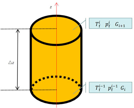
FIGURE 2. Sketch map of the short section of the production string.

Solution of the pressure profile inside the production string

Moreover, the gas properties also change in that the flow friction influences the wellbore pressure and temperature. The gas pressure can also be calculated, as expressed by Eq. 22:

$p_{\mathrm{f}}^i=p_{\mathrm{f}}^{i-1}-\left({\rho }_{\mathrm{f}}^{i}g\sin \theta +f^i\frac{{\rho }_{\mathrm{f}}^i{\left(v_{\mathrm{f}}^i\right)}^2}{2d_{\mathrm{t}\mathrm{n}}}\right)\Delta z-{\rho }_{\mathrm{f}}^i{v}_{\mathrm{f}}^i\Delta v_{\mathrm{f}}^i(22)$

where △v_f is the change of gas velocity in the short well section, m/s.

Because the well bottom temperature and pressure are available through well logging, the calculation starts from the well bottom, as expressed by Eq. 23.

$\{\begin{array}{l}{T}_{\mathrm{f}}^0=T_{\mathrm{b}},\\ p_{\mathrm{f}}^0=p_{\mathrm{b}},\\ △v_{\mathrm{f}}^0=0,\\ G_1=f\left(T_{\mathrm{f}}^0,p_{\mathrm{f}}^0\right)\end{array}(23)$

where T_b is the well bottom temperature, K; and p_b is the well bottom pressure, Pa.

Changing law of the temperature profile

Changing law under different factors

An HPHT gas well is selected from Ref. [40] as a case well to study the changing law. The basic parameters can be found in the reference. The temperature distributions in the production string under different influencing factors are shown in Figure 3. The detailed analysis is as follows:

1) Changing law under different production times. As shown in Figure 3A1, the temperature inside the production string decreases from the well bottom to the wellhead more and more quickly. According to Figure 3A2, the wellhead temperature increases as the production prolongs, but the increasing rate gradually decreases, and the increment value is not so large. For example, the wellhead temperatures are 358.33K, 361.77K, 364.56K, 365.73K, and 367.62K, respectively, under the production times of 10, 50, 200, 365, and 1000 days. This indicates that the largest temperature difference appears at the wellhead. Moreover, the changing rate of the temperature profile becomes slower and slower as the production continues. This means that the wellhead temperature would keep stable under normal production. However, the production histories of some gas wells showed that the wellhead temperature sometimes fluctuates remarkably. This situation may be caused by some incidents, such as reservoir energy depletion, production string block, or water invasion.

2) Changing law under different production rates. As shown in Figure 3B1, the whole temperature profile increases as the production increases. Alternatively, the temperature change becomes smaller and smaller as the well depth increases. Combining Figure 3B2, it can be observed that the maximum temperature change appears at the wellhead. For example, the wellhead temperatures are 349.85K, 365.73K, 390.77K, and 416.21K, respectively, under the production rates of 300 000 m³/d, 400 000 m³/d, 600 000 m³/d, and 800 000 m³/d, while the temperatures at the well bottom are equal. This can be explained by two reasons: first, a larger production rate brings more heat from the deep gas reservoir. Second, the heat generated by the flow friction increases. For some gas wells blocked by the wax deposition or the gas hydrate, the production rate can be increased in order to enhance the temperature profile of the gas wells.

3) Changing law under different values of the annular liquid thermal conductivity. The main function of the annular liquid is to prevent tubing collapse by balancing the pressure difference [41]. Meanwhile, the annular liquid also plays a role in thermal insulation by improving its thermal conductivity [42]. As shown in Figure 3C1, the annular liquid with higher thermal conductivity can enhance the temperature profile inside the production string. Similar to the impact of the annular liquid thermal conductivity, the maximum temperature change appears at the wellhead, but the trend is the opposite. Taking the wellhead temperature in Figure 3C2 as an example, the temperature increases from 358.58K to 374.42K when the annular liquid thermal conductivity decreases from 1.0 W/(mK) to 0.4 W/(mK). Hence, the annular liquid with low thermal conductivity can be applied to mitigate the trapped annular pressure. If necessary, the annular liquid thermal conductivity can be even lower, thus increasing the temperature profile. Likewise, this can also be used in the prevention of wax deposition or the gas hydrate block in low-temperature gas wells.

4) Changing law under different values of the gas-specific heat capacity. As shown in Figure 3D1, the temperature profile increases as the gas heat capacity increases. According to Figure 3D2, the wellhead temperature has an approximate positive linear relation with the gas-specific heat capacity, which is the same as the impact of the production rate. Since natural gas is compressible, the temperature has an impact on the heat capacity. Currently, there are several methods to express the impact of temperature on gas capacity, including the formula HYSYS software and API formula. However, these methods may not be applicable when the natural gas is mixed with different kinds of gas or the temperature is very high [43]. Therefore, the gas heat capacity should be tested in order to improve the calculation accuracy of temperature distribution in gas wells. On the other hand, the specific heat capacity of the production fluid would also change when the water enters the wellbore, thus leading to a change in the well temperature distribution.

FIGURE 3

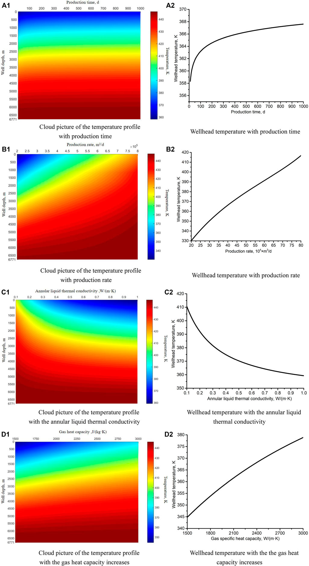
FIGURE 3. Changing law of the temperature profile under different factors. (A1) and (A2) are the impacts of production time. (B1) and (B2) are the impacts of production rate. (C1) and (C2) are the impacts of annular liquid thermal conductivity. (D1) and (D2) are the impacts of gas heat capacity.

Evaluation of the influencing factors

The wellhead is convenient to observe, so it can be taken as an index to reflect the wellbore temperature distribution and reservoir temperature. As stated previously, the changing law and the changing degree are different under the influences of different factors. Limited by the value ranges and the units of different factors, it is hard to directly compare the sensitivities of the influencing factors. For this reason, a new dimensionless index is proposed by Zhang et al. [44], which is called the ratio of standard deviation coefficient. To eliminate the impact of the factors’ units, this index is the ratio of the standard deviation coefficient of wellhead temperature and influencing factor. To eliminate the impact of the value range, it is necessary to get the starting point of the value range back to 0. Based on the two principles, the ratio of the standard deviation coefficient can be obtained in three steps. The first step is to get the starting point of the value range back to 0, as expressed by Eq. 24:

$x_j^{\prime }=x_{\mathrm{j}}-\min \left(x_1,x_2,x_3\dots \dots x_{\mathrm{n}}\right)(24)$

where $x_j^{\prime }$ is the jth value of the factor x after returning to 0; x_j is the jth value of the factor x; and n is the number of the factor values.

The second step is to calculate the standard deviation of the influencing factors and the wellhead temperature, as expressed by Eq. 25:

$\sigma =\sqrt{\frac{\sum _{j=1}^{j=n}{\left(x_j^{\prime }-x_{\mathrm{i}\mathrm{f}\mathrm{a}}\right)}^2}{\text{n}}}(25)$

where σ is the standard deviation and x_ifa is the average value of the factor value change.

Finally, the ratio of the standard deviation coefficient can be expressed by Eq. 26:

$C_{\mathrm{r}}=\frac{{\sigma }_{\mathrm{p}}{x}_{\text{ifa}}}{{\sigma }_{\mathrm{x}}{T}_{\mathrm{h}\mathrm{e}\mathrm{a}\mathrm{d}}}\times 100\%(26)$

where C_r is the ratio of the standard deviation coefficient, dimensionless; σ_p is the wellhead temperature standard deviation, K; σ_x is the standard deviation of the influencing factor; and T_head is the average value of the wellhead temperature, K.

Figure 4 shows the evaluation results. The sensitivity is presented by the new index, the ratio of the standard deviation coefficient. Here, the sensitivity in Figure 4 means the ability of the influencing factors to change the wellhead temperature. The higher the sensitivity is, the stronger the ability is. The horizontal axis represents the feasibility to adjust the wellhead temperature through the related factor. It can be seen that the gas-specific heat capacity has the highest sensitivity, while the production time has the lowest. Nevertheless, there are few methods to change the gas heat capacity in that this is a property determined by the production fluid. The production time can only be adjusted by stopping or continuing production. In other words, adjustment of the production time would disturb the production. The production rate can be adjusted through the oil nozzle. The only disadvantage is that the reservoir energy may be not able to last long at high production rate. The thermal conductivity of the annular liquid is easy to adjust by selecting different kinds of thermal-insulated liquids [45]. Given the cost, it is recommended to change the well temperature profile by adjusting the production rate. If not applicable, the thermal conductivity can be optimized to change the temperature profile.

FIGURE 4

FIGURE 4. Feasibility and sensitivity of the influencing factors.

Conclusion

1) The wellhead temperature increases as the production time increases, but the changing rate of the temperature profile becomes slower and slower as the production continues. Therefore, the obvious change in wellhead temperature can reflect potential production incidents of gas wells, such as reservoir energy depletion, production string block, or water invasion.

2) The production rate and annular liquid thermal conductivity can improve the temperature profile inside the production string, which can be used to prevent wax or hydrate deposition in gas wells with low temperature. The gas-specific heat capacity and temperature have a coupling relationship, so the changing law of gas-specific heat should be considered to improve the calculation accuracy.

3) Considering the sensitivity, feasibility, and cost, it is recommended to change the well temperature profile by adjusting the production rate. If not applicable, the thermal conductivity can be optimized to change the temperature profile.

Data availability statement

The original contributions presented in the study are included in the article/Supplementary Material; further inquiries can be directed to the corresponding author.

Author contributions

LC: data analysis, writing—original draft preparation, and methodology; JS: methodology, conceptualization, and supervision; BZ: writing—original draft preparation, funding acquisition, and supervision; NL: conceptualization, project administration, and drawing figures; YX: formal analysis.

Funding

This study received funding from CNPC Forward-looking Basic Strategic Technology Research Projects (Nos. 2021DJ6504, 2021DJ6502, 2021DJ6501, 2021DJ0806, and 2021DJ4902). The funder was not involved in the study design, collection, analysis, interpretation of data, writing of the manuscript, or the decision to submit it for publication.

Conflict of interest

Author LC was employed by Research Institute of Oil and Gas Engineering of Tarim Oilfield, PetroChina. Authors BZ were employed by Research Institute of Safety and Environment Technology, CNPC. Author NL was employed by Research Institute of Petroleum Exploration and Development, PetroChina.

The remaining authors declare that the research was conducted in the absence of any commercial or financial relationships that could be construed as a potential conflict of interest.

Publisher’s note

All claims expressed in this article are solely those of the authors and do not necessarily represent those of their affiliated organizations, or those of the publisher, the editors, and the reviewers. Any product that may be evaluated in this article, or claim that may be made by its manufacturer, is not guaranteed or endorsed by the publisher.

References

1. Fu W., Wang Z., Sun B., Xu J., Chen L., Wang X. Rheological properties of methane hydrate slurry in the presence of xanthan gum. SPE J (2020) 25(5):2341–52. doi:10.2118/199903-pa

CrossRef Full Text | Google Scholar

2. Fu W., Wang Z., Zhang J., Sun B. Methane hydrate formation in a water-continuous vertical flow loop with xanthan gum. Fuel (2020) 265:116963. doi:10.1016/j.fuel.2019.116963

CrossRef Full Text | Google Scholar

3. Zhang B., Jiang R., Sun B., Lu N., Hou J., Bai Y., et al. Establishment of the productivity prediction method of Class III gas hydrate developed by depressurization and horizontal well based on production performance and inflow relationship. Fuel (2022) 308:122006. doi:10.1016/j.fuel.2021.122006

CrossRef Full Text | Google Scholar

4. Gong W., You L., Xu J., Kang Y., Zhou Y. Experimental study on the permeability jail range of tight gas reservoirs through the gas–water relative permeability curve. Front Phys (2022) 695. doi:10.3389/fphy.2022.923762

CrossRef Full Text | Google Scholar

5. Lu N., Zhang B., Wang T., Fu Q. Modeling research on the extreme hydraulic extension length of horizontal well: Impact of formation properties, drilling bit and cutting parameters. J Pet Explor Prod Technol (2021) 11(3):1211–22. doi:10.1007/s13202-021-01106-4

CrossRef Full Text | Google Scholar

6. Vargo R. F., Payne M., Faul R., LeBlanc J., Griffith J. E. Practical and successful prevention of annular pressure buildup on the Marlin project. SPE drilling & completion (2003) 18(3):228–34. doi:10.2118/85113-pa

CrossRef Full Text | Google Scholar

7. Wang J., Sun J., Xie W., Chen H., Wang C., Yu Y., et al. Simulation and analysis of multiphase flow in a novel deepwater closed-cycle riserless drilling method with a subsea pump+ gas combined lift. Front Phys (2022) 565. doi:10.3389/fphy.2022.946516

CrossRef Full Text | Google Scholar

8. Cao L., Sun J., Zhang B. (2022). Safety control Technology of ultra-high pressure gas wells with annular pressure: Case study of Tarim Oilfield. Paper presented at the Offshore Technology Conference Asia. OTC-31458-MS Kuala Lumpur, Malaysia March 22-25. Dallas, United States. doi:10.4043/31458-MS

CrossRef Full Text | Google Scholar

9. Xu Y., Han C., Sun J., He B., Guan Z., Zhao Y. Formation interval determination method of MPD based on risk aversion and casing level optimization. Front Phys (2022) 734. doi:10.3389/fphy.2022.976379

CrossRef Full Text | Google Scholar

10. Moore T. A. Coalbed methane: A review. Int J Coal Geology (2012) 101:36–81. doi:10.1016/j.coal.2012.05.011

CrossRef Full Text | Google Scholar

11. Chen J., Wang X., Sun Y., Ni Y., Xiang B., Liao J. Factors controlling natural gas accumulation in the southern margin of junggar basin and potential exploration targets. Front Earth Sci (Lausanne) (2021) 9:112. doi:10.3389/feart.2021.635230

CrossRef Full Text | Google Scholar

12. Zhang B., Lu N., Guo Y., Wang Q., Cai M., Lou E. Modeling and analysis of sustained annular pressure and gas accumulation caused by tubing integrity failure in the production process of deep natural gas wells. J Energ Resour Tech (2022) 144(6):063005. doi:10.1115/1.4051944

CrossRef Full Text | Google Scholar

13. Ding L., Rao J., Xia C. Transient prediction of annular pressure between packers in high-pressure low-permeability wells during high-rate, staged acid jobs. Oil Gas Sci Technol – Rev IFP Energies Nouvelles (2020) 75:49. doi:10.2516/ogst/2020046

CrossRef Full Text | Google Scholar

14. Zhang B., Xu Z., Guan Z., Li C., Liu H., Xie J., et al. Evaluation and analysis of nitrogen gas injected into deepwater wells to mitigate annular pressure caused by thermal expansion. J Pet Sci Eng (2019) 180:231–9. doi:10.1016/j.petrol.2019.05.040

CrossRef Full Text | Google Scholar

15. Bradford D. W., Fritchie D. G., Gibson D. H., Gosch S. W., Pattillo P. D., Sharp J. W., et al. Marlin failure analysis and redesign: Part 1—description of failure. SPE Drilling & Completion (2004) 19(2):104–11. doi:10.2118/88814-pa

CrossRef Full Text | Google Scholar

16. Zhang B., Sun B., Deng J., Lu N., Zhang Z., Fan H., et al. Method to optimize the volume of nitrogen gas injected into the trapped annulus to mitigate thermal-expanded pressure in oil and gas wells. J Nat Gas Sci Eng (2021) 96:104334. doi:10.1016/j.jngse.2021.104334

CrossRef Full Text | Google Scholar

17. Li C., Guan Z., Zhao X., Yan Y., Zhang B., Wang Q., et al. A new method to protect the cementing sealing integrity of carbon dioxide geological storage well: An experiment and mechanism study. Eng Fracture Mech (2020) 236:107213. doi:10.1016/j.engfracmech.2020.107213

CrossRef Full Text | Google Scholar

18. Zhang B., Guan Z., Lu N., Hasan A. R., Xu S., Zhang Z., et al. (2018).Control and analysis of sustained casing pressure caused by cement sealed integrity failure. Paper presented at Offshore Technology Conference Asia held in. OTC-28500-MS Kuala Lumpur, Malaysia: doi:10.4043/28500-MS

CrossRef Full Text | Google Scholar

19. Li C., Guan Z., Zhang B., Wang Q., Xie H., Yan Y., et al. Failure and mitigation study of packer in the deepwater HTHP gas well considering the temperature-pressure effect during well completion test. Case Stud Therm Eng (2021) 26:101021. doi:10.1016/j.csite.2021.101021

CrossRef Full Text | Google Scholar

20. Mainguy M., Innes R. Explaining sustained A-annulus pressure in major North Sea high-pressure/high-temperature fields. SPE Drilling & Completion (2019) 34(1):71–80. doi:10.2118/194001-pa

CrossRef Full Text | Google Scholar

21. Ichim A., Teodoriu H. C. Investigations on the surface well cement integrity induced by thermal cycles considering an improved overall transfer coefficient. J Pet Sci Eng (2017) 154:479–87. doi:10.1016/j.petrol.2017.02.013

CrossRef Full Text | Google Scholar

22. Cao L., Sun J., Liu J., Liu J. Experiment and application of wax deposition in dabei deep condensate gas wells with high pressure. Energies (2022) 15(17):6200. doi:10.3390/en15176200

CrossRef Full Text | Google Scholar

23. Zhang J., Wang Z., Duan W., Fu W., Sun B., Sun J., et al. Real-time estimation and management of hydrate plugging risk during deepwater gas well testing. SPE J (2020) 25(6):3250–64. doi:10.2118/197151-pa

CrossRef Full Text | Google Scholar

24. Roberts B. E. The effect of sulfur deposition on gaswell inflow performance. SPE Reservoir Eng (1997) 12(02):118–23. doi:10.2118/36707-pa

CrossRef Full Text | Google Scholar

25. Mo L., Sun W., Jiang S., Zhao X., Ma H., Liu B., et al. Removal of colloidal precipitation plugging with high-power ultrasound. Ultrason Sonochem (2020) 69:105259. doi:10.1016/j.ultsonch.2020.105259

PubMed Abstract | CrossRef Full Text | Google Scholar

26. Wang Z., Tong S., Wang C., Zhang J., Fu W., Sun B. Hydrate deposition prediction model for deep-water gas wells under shut-in conditions. Fuel (2020) 275:117944. doi:10.1016/j.fuel.2020.117944

CrossRef Full Text | Google Scholar

27. Izgec B., Kabir C. S., Zhu D., Hasan A. R. Transient fluid and heat flow modeling in coupled wellbore/reservoir systems. SPE Reservoir Eval Eng (2007) 10(3):294–301. doi:10.2118/102070-pa

CrossRef Full Text | Google Scholar

28. Galvao M. S., Carvalho M. S., Barreto A. B. A coupled transient wellbore/reservoir-temperature analytical model. SPE J (2019) 24(5):2335–61. doi:10.2118/195592-pa

CrossRef Full Text | Google Scholar

29. Wang X., Sun B., Liu S., Zhong L., Liu Z., Wang Z., et al. A coupled model of temperature and pressure based on hydration kinetics during well cementing in deep water. Pet Exploration Dev (2020) 47(4):867–76. doi:10.1016/s1876-3804(20)60102-1

CrossRef Full Text | Google Scholar

30. Mao L., Liu Q., Nie K., Wang G. Temperature prediction model of gas wells for deep-water production in South China Sea. J Nat Gas Sci Eng (2016) 36:708–18. doi:10.1016/j.jngse.2016.11.015

CrossRef Full Text | Google Scholar

31. Guan Z. C., Zhang B., Wang Q., Liu Y. W., Xu Y. Q., Zhang Q. Design of thermal-insulated pipes applied in deepwater well to mitigate annular pressure build-up. Appl Therm Eng (2016) 98:129–36. doi:10.1016/j.applthermaleng.2015.12.030

CrossRef Full Text | Google Scholar

32. Hasan A. R., Kabir C. S., Lin. D. Analytic wellbore temperature model for transient gas-well testing. SPE Reservoir Eval Eng (2005) 8(3):240–7. doi:10.2118/84288-pa

CrossRef Full Text | Google Scholar

33. Zheng J., Dou Y. H., Cao Y., Yan X. Prediction and analysis of wellbore temperature and pressure of HTHP gas wells considering multifactor coupling. J Fail Anal Preven (2020) 20(1):137–44. doi:10.1007/s11668-020-00811-2

CrossRef Full Text | Google Scholar

34. Ai S., Cheng L., Huang S., Liu H., Zhang J., Fu L. A critical production model for deep HT/HP gas wells. J Nat Gas Sci Eng (2015) 22:132–40. doi:10.1016/j.jngse.2014.11.025

CrossRef Full Text | Google Scholar

35. Ramey H. J.. Wellbore heat transmission. J Pet Tech (1962) 14(4):427–35. doi:10.2118/96-pa

CrossRef Full Text | Google Scholar

36. Holst P. H., Flock D. L. Wellbore behaviour during saturated steam injection. J Can Pet Tech (1966) 5(04):184–93. doi:10.2118/66-04-05

CrossRef Full Text | Google Scholar

37. Hasan A. R., Kabir C. S., Wang X. A robust steady-state model for flowing-fluid temperature in complex wells. SPE Prod Operations (2009) 24(2):269–76. doi:10.2118/109765-pa

CrossRef Full Text | Google Scholar

38. Thome J. R., Ribatski G. State-of-the-art of two-phase flow and flow boiling heat transfer and pressure drop of CO2 in macro-and micro-channels. Int J Refrigeration (2005) 28(8):1149–68. doi:10.1016/j.ijrefrig.2005.07.005

CrossRef Full Text | Google Scholar

39. Heidaryan E., Salarabadi A., Moghadasi J. A novel correlation approach for prediction of natural gas compressibility factor. J Nat Gas Chem (2010) 2(18):189–92. doi:10.1016/s1003-9953(09)60050-5

CrossRef Full Text | Google Scholar

40. Zhang B., Xu Z., Lu N., Liu H., Liu J., Hu Z., et al. Characteristics of sustained annular pressure and fluid distribution in high pressure and high temperature gas wells considering multiple leakage of tubing string. J Pet Sci Eng (2021) 196:108083. doi:10.1016/j.petrol.2020.108083

CrossRef Full Text | Google Scholar

41. Liu H., Cao L., Xie J., Yang X., Zeng N., Zhang X., Chen F. (2019). Research and practice of full life cycle well integrity in HTHP well, Tarim Oilfield. Paper presented at International Petroleum Technology Conference. Beijing, China. Dallas, United States IPTC-19403-MS doi:10.2523/IPTC-19403-MS

CrossRef Full Text | Google Scholar

42. Ezzat A. M., Miller J. J., Ezell R., Perez G. P. (2007). High-performance water-based insulating packer fluids. Paper presented at SPE Annual Technical Conference and Exhibition. SPE-109130-MS Anaheim, CA, USA. Dallas, United States.

Google Scholar

43. Yuan W., Yang W., Liao T., Ma Y. Comparative study on equations of ideal gas specific heat capacity. Pet Eng Construction (2021) 47(2):25–9. doi:10.3969/j.issn.1001-2206.2021.02.006

CrossRef Full Text | Google Scholar

44. Zhang B., Guan Z., Sheng Y., Wang Q., Xu C. Impact of wellbore fluid properties on trapped annular pressure in deepwater wells. Pet Exploration Dev (2016) 43(5):869–75. doi:10.1016/s1876-3804(16)30104-5

CrossRef Full Text | Google Scholar

45. Zhang B., Guan Z., Wang Q., Xuan L., Liu Y., Sheng Y. (2016). Appropriate completion to prevent potential damage of annular pressure buildup in deepwater wells. Paper presented at IADC/SPE Asia Pacific Drilling Technology Conference. Singapore. Dallas, United States SPE-180542-MS doi:10.2118/180542-MS

CrossRef Full Text | Google Scholar