BUQEYE guide to projection-based emulators in nuclear physics

1 Introduction

Nuclear systems are notoriously complex. But typically, our theoretical modeling of nuclear phenomena contains superfluous information for quantities of interest. Model order reduction (MOR) refers to powerful techniques that enable us to reduce a system’s complexity systematically (e.g., see Refs. [1–3] for comprehensive introductions). These techniques enable emulators, which are low-dimensional surrogate models capable of rapidly and reliably approximating high-fidelity models, making practical otherwise impractical calculations. But the nuclear physics community has barely scratched the surface of the types of emulators that could be crafted or explored their full range of applications.

A fertile area for new emulators is uncertainty quantification (UQ) [4–13] in nuclear physics, which is the general theme of this Frontiers Research Topic [14]. Quantifying theoretical uncertainties rigorously is crucial for comparing theory predictions with experimental and/or observational constraints and performing model comparison and/or mixing [15]. However, UQ has only recently drawn much attention as nuclear theory has entered the precision era. Bayesian parameter estimation for nuclear effective field theory (EFT) and optical models, UQ for nuclear structure pushing toward larger masses and for reactions across the chart of nuclides, experimental design [15–17] for the next-generation of precision experiments probing the nuclear dripline, and many other applications will all benefit from emulators. This Research Topic [14] already contains several new applications of emulators for nuclear physics. Key to the wider adoption of these tools is the evangelization of their potential and the creation of pedagogical guides for those first starting in this field [18]. This article is aimed at both goals.

To do so, the BUQEYE collaboration (Bayesian Uncertainty Quantification: Errors in Your EFT) [19] has created a rather unconventional document comprised of the article you are reading now along with a companion website [20] containing interactive supplemental material and source code that generates all the results shown, and much more. Interested individuals can dynamically generate different versions of this document based on tunable parameters. We hope that this format encourages readers to experiment and build upon the examples presented here, thereby facilitating new applications.

Various types of emulators have already been applied with success within nuclear physics. A non-exhaustive list of applications includes Refs. [7, 9, 21–42]. But as emphasized in Refs. [18, 43], there is a broad and relatively mature MOR literature outside of nuclear physics waiting to be exploited (e.g., see Ref. [44] for an overview of the Universe of MOR approaches). Our goal in this guide will be to facilitate this exploitation through a selective treatment of physics-informed, projection-based emulators relevant to a wide range of nuclear physics problems.

To this end, we organize this guide as follows. Section 2 focuses on emulators for bound-state calculations using subspace-projection methods. We then provide a more general introduction to MOR for solving differential equations in Section 3, which leads to our discussion of scattering emulators in Section 4. Section 5 concludes with a summary and outlook. Throughout, we draw connections between variational and Galerkin projection methods and illustrate these concepts with pedagogical examples, supplemented by source code on the companion website [20].

2 Eigen-emulators

In this section, we discuss the construction of fast and accurate emulators for bound-state calculations. Given a (Hermitian) Hamiltonian H(θ) parameterized by $\mathit{\theta }$, we aim to find the solutions {E(θ), |ψ(θ)⟩} of the Schrödinger Equation

$H\left(\mathit{\theta }\right)|\psi \left(\mathit{\theta }\right)\rangle =E\left(\mathit{\theta }\right)|\psi \left(\mathit{\theta }\right)\rangle ,(1)$

subject to the normalization ⟨ψ(θ)|ψ(θ)⟩ = 1. The components of the vector θ may be model parameters, such as the low-energy couplings of a nuclear EFT, or other parameters describing the system of interest [33, 40]. We consider here cases in which Eq. 1 can be solved with high fidelity, but doing so requires a significant amount of compute time. This compute time is compounded when repeated solutions are required throughout the parameter space, e.g., during optimization routines or Monte Carlo sampling. In the following, we will discuss how the Ritz variational principle and the Galerkin method can be used to construct rapid and reliable¹ emulators that facilitate these calculations.

2.1 Variational approach

To construct an emulator for bound state calculations, we use here the Rayleigh–Ritz method² and thus consider the energy functional

$\mathcal{E}\left[\tilde{\psi }\right]=⟨\tilde{\psi }|H\left(\mathit{\theta }\right)|\tilde{\psi }⟩-\tilde{E}\left(\mathit{\theta }\right)\left(⟨\tilde{\psi }|\tilde{\psi }⟩-1\right),(2)$

where the Lagrange multiplier $\tilde{E}(\mathit{\theta })$ (also known as Ritz value) imposes the normalization condition $⟨\tilde{\psi }|\tilde{\psi }⟩=1$ for bound states. The Generalized Ritz Theorem [47]³ states that the functional (Eq. 2) is stationary about all (discrete) solutions of the Eq. 1, not just the ground state solution, which can be seen by imposing the stationary condition

$\delta \mathcal{E}\left[\tilde{\psi }\right]\equiv 0=2⟨\delta \tilde{\psi }|\left[H\left(\mathit{\theta }\right)-\tilde{E}\left(\mathit{\theta }\right)\right]|\tilde{\psi }⟩-\delta \tilde{E}\left(\mathit{\theta }\right)\left[⟨\tilde{\psi }|\tilde{\psi }⟩-1\right],(3)$

and noting that Eq. 3 is only fulfilled for arbitrary variations $\langle \delta \tilde{\psi }|$ if $|\tilde{\psi }\rangle$ is a solution of the Schrödinger Eq. 1 with $\tilde{E}(\mathit{\theta })=E(\mathit{\theta })$.

Let us now define the trial wave function we use in conjunction with the functional (2):

$|\tilde{\psi }\rangle =\sum _{i=1}^{n_b}{\beta }_i|{\psi }_i\rangle \equiv X\vec{\beta },(\mathrm{4a})$

$X=\left[\begin{array}{cccc}\hfill |{\psi }_1\rangle \hfill & \hfill |{\psi }_2\rangle \hfill & \hfill \cdots \hfill & \hfill |{\psi }_{n_b}\rangle \hfill \end{array}\right],(\mathrm{4b})$

where the column-vector $\vec{\beta }$ contains the to-be-determined coefficients and the row-vector ⁴ X the (in principle) arbitrary basis states. Here, we use snapshots of high-fidelity solutions of the Eq. 1 at a set of given parameter values; i.e., ${\{|{\psi }_i\rangle \equiv |\psi ({\mathit{\theta }}_i)\rangle \}}_{i=1}^{n_b}$ [2, 48–50]. No assumption has been made as to how to obtain the high-fidelity solutions.

Figure 1 motivates the efficacy of snapshot-based trial functions. Although a given eigenvector |ψ(θ)⟩ obtained from a high-fidelity solver resides in a high-dimensional (or even infinite-dimensional) space, the trajectory traced out by continuous variations in θ remains in a relatively low-dimensional subspace (as illustrated by the gray plane). Hence, linear combinations of high-fidelity eigenvectors spanning this subspace (i.e., the snapshots) make extremely effective trial wave functions for variational calculations. In nuclear physics, snapshot-based emulators already have accurately approximated ground-state properties, such as binding energies, charge radii [7, 9, 25], and transition matrix elements [9, 29], and have been explored for applications to excited states [51].

FIGURE 1

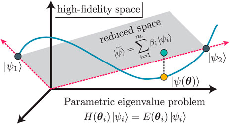
FIGURE 1. Illustration of a projection-based emulator using only two snapshots |ψ_i⟩ ≡ |ψ(θ_i)⟩ (dark gray points). These snapshots are high-fidelity solutions of the Schrödinger Eq. 1, which span the subspace of the reduced-order model, as indicated by the red arrows and the gray plane. The trajectory of a high-fidelity eigenvector is denoted by the blue curve. The orange dot depicts an eigenvector |ψ(θ)⟩ along the trajectory that, when projected onto the reduced space, corresponds to the turquoise point; hence, the difference between the orange and turquoise points represents the error due to the emulator’s subspace projection (i.e., the dotted line). Inspired by Figure 2.1 in Ref. [2].

Given the trial wave function (4), we determine the coefficients ${\vec{\beta }}_{\star }$ that render $\mathcal{E}[\tilde{\psi }=X\vec{\beta }]$ stationary under variations $|\delta \tilde{\psi }\rangle =X|\delta \vec{\beta }\rangle$ of the trial wave function, as opposed to arbitrary variations. Solving for the optimal ${\vec{\beta }}_{\star }$ occurs then in the low-dimensional space spanned by the basis elements in X (i.e., the red arrows in Figure 1) rather than in the high-dimensional space in which |ψ⟩ resides. From the stationarity condition Eq. 3, we obtain the reduced-order model [52],

$\tilde{H}\left(\mathit{\theta }\right){\vec{\beta }}_{\star }\left(\mathit{\theta }\right)=\tilde{E}\left(\mathit{\theta }\right)\tilde{N}{\vec{\beta }}_{\star }\left(\mathit{\theta }\right),(\mathrm{5a})$

${\vec{\beta }}_{\star }^{†}\left(\mathit{\theta }\right)\tilde{N}{\vec{\beta }}_{\star }\left(\mathit{\theta }\right)=1,(\mathrm{5b})$

where $\tilde{H}(\mathit{\theta })\equiv X^{†}H(\mathit{\theta })X$ is the subspace-projected Hamiltonian and $\tilde{N}\equiv X^{†}X$ the norm matrix in the snapshot basis. As opposed to H(θ) in Eq. 1, $\tilde{H}(\mathit{\theta })$ (and likewise $\tilde{N}$) is a n_b × n_b Hermitian matrix,

$\tilde{H}\left(\mathit{\theta }\right)=\left[\begin{array}{ccc}\hfill ⟨{\psi }_1|H\left(\mathit{\theta }\right)|{\psi }_1⟩\hfill & \hfill \cdots \hfill & \hfill ⟨{\psi }_1|H\left(\mathit{\theta }\right)|{\psi }_{n_b}⟩\hfill \\ \hfill ⋮\hfill & \hfill \ddots \hfill & \hfill ⋮\hfill \\ \hfill ⟨{\psi }_{n_b}|H\left(\mathit{\theta }\right)|{\psi }_1⟩\hfill & \hfill \cdots \hfill & \hfill ⟨{\psi }_{n_b}|H\left(\mathit{\theta }\right)|{\psi }_{n_b}⟩\hfill \end{array}\right].(6)$

In practice, the generalized eigenvalue problem Eq. 5 may experience numerical instabilities due to small singular values in $\tilde{N}$. (The instabilities also appear in reduced-order modeling of differential equations, see Section 3). One way to ameliorate these instabilities is to orthonormalize the snapshots in X, hence yielding $\tilde{N}=\mathbb{1}$. This approach could also permit some efficiency gains, by excluding the least important vectors as measured by their singular values. Alternatively, Ref. [53] recently introduced a trimmed sampling algorithm that can substantially reduce the effects of noise in solving generalized eigenvalue problems. Finally, a well-known approach to regularize both generalized eigenvalue problems and matrix inversion is through the use of a nugget [54, 55]. Here, a regularization parameter ν ≪ 1 (called a nugget) is added to the diagonal of the ill-conditioned matrix one wishes to invert (here, $\tilde{N}$), thus shifting its singular values.

By solving the generalized eigenvalue problem Eq. 5, one obtains n_b pairs $\{\tilde{E}(\mathit{\theta }),{\vec{\beta }}_{\star }(\mathit{\theta })\}$ consisting of a Lagrange multiplier (i.e., an eigenvalue) and its corresponding coefficient vector. Let us index the eigenvalues of the Eq. 5 and Eq. 1 in ascending order; that is, ${\tilde{E}}_n⩽{\tilde{E}}_{n+1}$ and E_n⩽E_n+1, respectively, with n = 1 indicating the lowest eigenvalue. If the snapshot basis X in the trial wave function (Eq. 4) contains n_b linearly independent states, then the Min–Max Theorem [47] asserts that each Lagrange multiplier,

${\tilde{E}}_n\left(\mathit{\theta }\right)⩾E_n\left(\mathit{\theta }\right)\text{for}1⩽n⩽n_b,(7)$

provides an upper bound on its corresponding eigenvalue of the Schrödinger Eq. 1.⁵ Furthermore, the Generalized Ritz Theorem implies that the ${\tilde{E}}_n(\mathit{\theta })$ provide not only the variational bounds (Eq. 7) but also stationary approximations for these high-fidelity eigenvalues. Adding another basis state to X can only improve these approximations, which converge to the high-fidelity eigenvalues as the projected subspace approaches the high-fidelity space [47].

Although excited states can also be emulated, especially when adding excited-state snapshots to the trial wave function to improve the emulator’s accuracy (see also Ref. [51]), we focus on ground-state properties and thus use only ground-state snapshots in the trial wave function. For brevity, we will omit the subscripts henceforth. To obtain the approximate ground-state wave function associated with $\tilde{E}(\mathit{\theta })$, one evaluates the Ritz vector $|\psi (\mathit{\theta })\rangle \hspace{0.17em}\approx X{\vec{\beta }}_{\star }(\mathit{\theta })$. Expectations values of operators O can then be straightforwardly computed using

$⟨\psi \left(\mathit{\theta }\right)|O\left(\mathit{\theta }\right)|\psi \left(\mathit{\theta }\right)⟩\approx {\vec{\beta }}_{\star }^{†}\left(\mathit{\theta }\right)\tilde{O}{\vec{\beta }}_{\star }\left(\mathit{\theta }\right),(8)$

with the subspace-projected $\tilde{O}(\mathit{\theta })=X^{†}O(\mathit{\theta })X$. However, these expectation values generally do not provide variational bounds unless O = H is the Hamiltonian, as discussed (see, e.g., Figure 5 in Ref. [25] for emulated ⁴He ground-state radii).

2.2 Galerkin approach

The reduced-order model (5) can be alternatively derived via a Galerkin projection, as we will also see with the variational emulators for scattering in Section 4. To this end, we construct the weak form of the Eq. 1 by left-multiplying it by an arbitrary test function ⟨ζ| and asserting that

$⟨\zeta |H\left(\mathit{\theta }\right)-E\left(\mathit{\theta }\right)|\psi ⟩=0,\forall \langle \zeta |.(9)$

If the weak form (9) is satisfied for all ⟨ζ| for a given set {E, |ψ⟩}, then the set must also satisfy the Eq. 1. The proof of this statement can be obtained via a contrapositive: if Eq. 1 were not satisfied, then one could find a ⟨ζ| such that Eq. 9 is nonzero.

The weak form of the high-fidelity system is the starting point for deriving a reduced-order model. Although Eq. 9 still operates in the large space in which |ψ⟩ resides (cf. Figure 1), we can reduce its dimension by replacing $|\psi \rangle \to |\tilde{\psi }\rangle$, where $|\tilde{\psi }\rangle$ is defined in Eq. 4. With the degrees of freedom for |ψ⟩ reduced, we enforce a less strict orthogonality condition: we select n_b test functions ζ_i and assert that the residual due to the trial wave function (cf. Figure 1) should be orthogonal to the subspace $\mathcal{Z}$ spanned by these test functions $Z=[|{\zeta }_1\rangle ,\dots ,|{\zeta }_{n_b}\rangle ]$:

$\left(H\left(\mathit{\theta }\right)-\tilde{E}\left(\mathit{\theta }\right)\right)|\tilde{\psi }\rangle \perp \mathcal{Z},(10)$

or likewise

$⟨\zeta |H\left(\mathit{\theta }\right)-\tilde{E}\left(\mathit{\theta }\right)|\tilde{\psi }⟩=0,\forall |\zeta \rangle \in \mathcal{Z}.(11)$

But replacing $|\psi \rangle \to |\tilde{\psi }\rangle$ also implies that the true eigenvalue E is in general not exactly reproduced unless $\mathcal{X}$ contains |ψ(θ)⟩. Hence, we also had to apply the approximation $\tilde{E}\approx E$ in Eqs. 10 and 11.

In the Galerkin method, which is also known as the “method of weighted residuals,” the test and trial function bases are chosen to be equivalent; i.e., $\mathcal{Z}=\mathcal{X}$. The so-called Galerkin condition Eq. 11 is then equivalent to imposing that $⟨{\psi }_i|H-\tilde{E}|\tilde{\psi }⟩=0$ holds for i ∈ [1, n_b]. This yields a system of n_b equations with n_b unknowns $\vec{\beta }$ and, together with the normalization condition, reduces to Eq. 5 obtained from the variational principle in Section 2.1. However, we stress that the test and trial function bases can be chosen differently (i.e., |ζ_i⟩ ≠ |ψ_i⟩), which makes the Galerkin method more general than the variational approach. Note that the normalization condition does not affect the Galerkin condition Eq. 11 and can be implemented by normalizing the trial function.

2.3 Emulator workflow and offline-online decomposition

Figure 2 illustrates the workflow for implementing fast and accurate emulators as described in Section 2.1. The workflow involves

1. a computational framework capable of reliably solving the high-fidelity system Eq. 1,

2. the snapshot-based trial wave function Eq. 4 with the optimal coefficients (i.e., the weights) determined by the Eq. 5, and

3. an efficient offline-online decomposition in which the computational heavy lifting is performed once before the emulator is invoked.

FIGURE 2

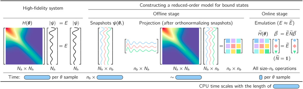
FIGURE 2. Illustration of the workflow for implementing fast and accurate emulators, including a high-fidelity solver (left) and an intrusive, projection-based emulator with efficient offline-online decomposition (right), for sampling the (approximate) solutions of the Schrödinger Eq. 1 in the parameter space θ. For brevity, the figure assumes that the snapshots are orthonormalized during the offline stage such that $\tilde{N}=\mathbb{1}$ in the emulator Eq. 5. See the main text for details.

Several computational frameworks exist in nuclear physics (and quantum chemistry) for solving the few- and many-body Schrödinger Eq. 1 [56]. For illustration, Figure 2 assumes that the high-fidelity solver performs a direct diagonalization of the N_h × N_h Hamiltonian in a chosen (truncated) model basis of length N_h. The corresponding runtime t_s per sampling point θ_i is indicated by the width of the blue bar in Figure 2. In nuclear physics, such approaches are referred to as Configuration Interaction (CI). However, the following discussion will be independent of how the high-fidelity solutions of the Eq. 1 are obtained in practice.

Using the high-fidelity solver, one constructs a set of snapshots ${\{|\psi ({\mathit{\theta }}_i)\rangle \}}_{i=1}^{n_b}$ in the truncated model basis to build the columns of the N_h × n_b matrix X. The runtime for this task is n_b × t_s. For simplicity, Figure 2 assumes n_b = 3 and depicts the basis functions schematically in different colors. This phase of the emulator needs to be completed only once before the emulator is invoked and is thus called the offline stage as opposed to the online stage of the emulator. The predictions are made quickly and with little memory footprint in the online stage.

The appearance of the full-order Hamiltonian during the offline stage, where the projected Hamiltonian $\tilde{H}(\mathit{\theta })\equiv X^{†}H(\mathit{\theta })X$ is computed (see Figure 2), implies that this class of projection-based emulators is intrusive in nature. In general, intrusive emulators apply the basis expansions and projections to the operators implemented in the high-fidelity model [57]. On the other hand, non-intrusive emulators use only outputs of the full-order solver without access to the full-order operators such as the Hamiltonian. Non-intrusive emulators include Gaussian processes [58], Dynamic Mode Decompositions [59, 60], and other machine learning methods [61–63]. More details on this classification scheme can be found in Section 8 in Ghattas and Willcox [57].

The emulator’s efficiency greatly benefits from moving all size-N_h operations into the offline stage, which can easily be achieved for Hamiltonians H(θ) with an affine parameter dependence. These affine operators can be written as a sum of products of parameter-dependent functions $h_n(\mathit{\theta })$ and parameter-independent operators $H_n$,

$H(\mathit{\theta })=\sum _n{h}_n(\mathit{\theta })H_n.(12)$

Note that the functions h_n(θ) are only required to be smooth but not necessarily linear in θ. The affine parameter dependence in Eq. 12 then allows one to store the subspace-projected operators ${\tilde{H}}_n=X^{†}{H}_{n}X$ separately up front in the offline phase, from which

$\tilde{H}\left(\mathit{\theta }\right)=\sum _n{h}_n\left(\mathit{\theta }\right){\tilde{H}}_n,(13)$

can be efficiently constructed for each θ_i during the online stage to solve the emulator equation 5. For instance, Hamiltonians derived from chiral EFT can be cast into the form (12) due to their affine dependence on the low-energy couplings. The runtime per sample θ_i in the online phase is therefore typically just a small fraction of that of the high-fidelity solver, as depicted by the small blue box in Figure 2. Likewise, emulating expectation values of other operators with an affine parameter dependence via Eq. 8 also benefits from this offline-online decomposition. For non-affine operators, various hyperreduction methods have been developed to construct approximate affine representations [50, 64], including the empirical interpolation (EIM) [65–68] and gappy proper orthogonal decomposition [69, 70]. See also Refs [48, 71–73] for hyperreduction methods that interpolate X or $\tilde{H}(\mathit{\theta })$ directly, and Refs [33, 74] for recent applications of machine learning tools for hyperreduction.

How should one choose the snapshots in the trial wave function Eq. 4 effectively? For relatively small parameter spaces, one can use Latin hypercube sampling to obtain space-filling snapshots or choose the snapshots in the proximity of the to-be-emulated parameter ranges, keeping n_b ≪ N_h in practice. A chosen set of snapshots expressed in the (truncated) model basis can be optimized by applying a singular value decomposition (SVD) or the closely related proper orthogonal decomposition (POD) [75] to the N_h × n_b matrix X. One then creates a new set of snapshots from the (orthonormal) left-singular vectors associated with the singular values greater than a chosen threshold [64]. This (optional) preprocessing step can be performed during the offline stage, as illustrated in Figure 2, thereby rendering the Eq. 5 an eigenvalue problem (i.e., $\tilde{N}=\mathbb{1}$) and less sensitive to numerical noise.

The basis states of the trial wave function can also be obtained iteratively, using a greedy algorithm [64, 76, 77]. These algorithms estimate and then minimize the emulator’s overall error by adding basis states (obtained from a high-fidelity solver) in the parameter space where the error is expected to be the largest. Greedy algorithms require fast approximations of the emulator’s error and terminate when either a requested error tolerance or a maximum number of iterations has been achieved. Uncertainty quantification for reduced-order models has been studied in various contexts, including differential equations [64, 77, 78] and nuclear physics problems [24, 43].

2.4 Illustrative example

The formal results so far in this Section can be illuminated by a simple example, which allows us to compare results from a snapshot-based emulator to more conventional approaches, such as direct diagonalization in a harmonic oscillator basis and Gaussian process emulation. Let us define the system we would like to solve as a single particle with zero angular momentum in three dimensions and trapped in an anharmonic oscillator potential. This example can be directly generalized to few- and many-body systems. The potential operator is the sum of a conventional harmonic oscillator (HO) potential and a finite-range piece:

$V\left(r;\mathit{\theta }\right)=V_{\text{HO}}\left(r\right)+\sum _{n=1}^3{\theta }_n\exp \left(-r^2/{\sigma }_n^2\right),(14)$

with σ_n = [0.5, 2, 4] fm. The potential Eq. 14 has the affine structure defined in Eq. 12 for θ and hence can be emulated rapidly after projecting into the snapshot basis during the offline stage. Even the high-fidelity system considered here is still small enough to be solved quickly and accurately using a fine radial mesh on a standard laptop. However, this provides an illuminating setting within which we can observe many qualities seen in more complicated scenarios.

Following the MOR paradigm, we take snapshots of the high-fidelity wave function at various training parameters {θ_i} and collect them into our basis X. Here, we choose n_b = 6 training points randomly and uniformly distributed in the range [−5, 5] MeV for all θ_n; 50 validation parameter sets are chosen within the same range. The snapshots and the corresponding potentials are shown in Figure 3. These snapshots are then used to construct the reduced-order system as in Eq. 5. All of this, and more, is made simple by the EigenEmulator Python class provided in the supplemental material [20].

FIGURE 3

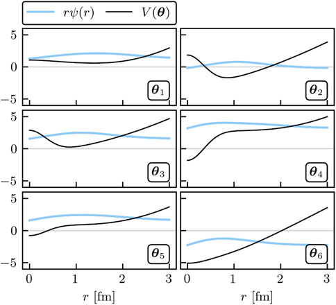
FIGURE 3. Basis functions for training the snapshot-based eigen-emulator. The black curves show the potential, and the blue curves show the wave functions as functions of the radial coordinate r. The wave functions are offset vertically by their corresponding energies for clarity. See the main text for details.

Once the reduced system has been constructed and the affine structure of the Hamiltonian exploited to store the projected matrices during the offline stage, we can begin rapid emulation during the online stage. To help provide a baseline to a common approach in nuclear physics, we provide an emulator constructed with the first n_b = 6 HO wave functions as the trial basis X in Eq. 5. We label this approach the HO emulator and the snapshot-based approach the reduced-basis method (RBM) emulator. See Ref. [18] for a guide to the extensive literature on RBMs. One can emulate quantities with this HO approach via our OscillatorEmulator class [20].

For example, we take three of the validation parameter sets we sampled and compare the exact and emulated wave functions for both emulators. Figure 4 shows the results. The gray lines depict the n_b wave functions used to create the reduced-order models, and the colored lines show the emulated results on top of the high-fidelity solutions (black lines). Although both the reduced basis and HO basis are rich enough to capture the main effects of varying θ, the RBM emulator is much more effective at capturing the fine details of the wave function. This can be seen in more detail in Figure 5, where the absolute residuals of the RBM emulator are orders of magnitude smaller than those of the HO emulator. The sensitivity of the emulator accuracy as n_b is varied can be readily studied using the Python code provided on the companion website [20].

FIGURE 4

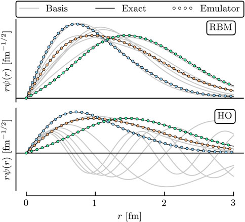
FIGURE 4. Emulated wave functions for the RBM emulator (top panel) and HO emulator (bottom panel) as a function of the radius. The solid black lines represent the exact solution, and the dots represent the emulator result. The gray lines give the wave functions used to train the emulator. See the main text for details.

FIGURE 5

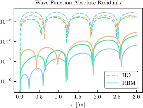
FIGURE 5. Absolute residuals of the emulated wave functions (in fm^−1/2) based on the RBM and HO emulator as a function of r, with colors corresponding to those in Figure 4. The emulator results are compared to the exact solutions. See the main text for details.

The quality of the emulators can be understood by noting in Figure 4 that the basis functions of the RBM emulator match much more closely with the emulated wave functions than the HO emulator, whose wave functions have nodes not seen in the ground state (see the gray lines). Thus, although the HO basis functions may be better at spanning the space of all possible wave functions, they are, in fact, a poor basis for spanning the set of all possible ground states as θ are varied. The RBM emulator constructs an extremely effective basis almost automatically, with minimal input required by the modeler. This can prove particularly effective for cases where the system’s complexity limits the quality of the basis that can be constructed from intuition or expertise alone.

Next, we discuss the emulation of bound-state observables. Straightforward to emulate are the eigen-energies E(θ), whose emulated values $\tilde{E}(\mathit{\theta })$ are the result of solving the Eq. 5. But as discussed in Section 2.1, other observables associated with the operator O can be emulated via $⟨\psi (\mathit{\theta })|O|\psi (\mathit{\theta })⟩\approx ⟨\tilde{\psi }(\mathit{\theta })|O|\tilde{\psi }(\mathit{\theta })⟩$ using the $\tilde{\psi }(\mathit{\theta })$ found from Eq. 5. We choose to show the results of emulating the radius-squared operator R², defined here to be

$⟨\psi |R^2|\psi ⟩=\frac{1}{\mathcal{N}}{\int }_0^{\infty }{r}^2\mathrm{d}r{r}^2{\psi }^2\left(r\right),(15)$

with the normalization $\mathcal{N}={\int }_0^{\infty }{r}^2\mathrm{d}r{\psi }^2(r)$. As stated previously, the bulk of the numerical effort in the evaluation of this matrix element is handled during the offline stage, where the integration is performed once,

${\tilde{R}}_{ij}^2\equiv ⟨{\psi }_i|R^2|{\psi }_j⟩=\frac{1}{\mathcal{N}}{\int }_0^{\infty }{r}^2\mathrm{d}r{r}^2{\psi }_i\left(r\right){\psi }_j\left(r\right),(16)$

and then the online stage emulation can occur quickly via Eq. 8; i.e., $⟨\psi (\mathit{\theta })|R^2|\psi (\mathit{\theta })⟩\approx {\sum }_{ij}{\vec{\beta }}_{\star }^{(i)}(\mathit{\theta }){\tilde{R}}_{ij}^2{\vec{\beta }}_{\star }^{(j)}(\mathit{\theta })$.

For illustrative purposes, we continue our example using the trained RBM and HO emulators, but add a popular emulation tool to the discussion: Gaussian processes (GPs). GPs are non-parametric, non-intrusive machine learning models for both regression and classification tasks [58, 79, 80]. Their popularity stems partly from their convenient analytical form and flexibility in effectively modeling various types of functions. GPs benefit from treating the underlying set of codes as a black box [57]; as we will soon see, this is a double-edged sword. We employ two independent GPs to emulate the ground-state energy and the corresponding radius expectation value. Each GP uses a Gaussian covariance kernel and is fit to the observable values at the same values of θ_i used to train the RBM emulator. We use the maximum likelihood values for the hyperparameters.

The absolute residuals at the validation points for each of the RBM, HO, and GP emulators are shown in Figures 6 and 7 for the energy and radius, respectively. Among these emulators, the GP emulators perform the worst, despite being trained on the values of the energies and radii themselves to perform this very emulation task. Furthermore, its ability to extrapolate beyond the support of its training data is often poor unless great care is taken in the design of its kernel and mean function (see Figures 1 and 2 in Ref. [25]). The GP suffers from what, in other contexts, could be considered its strength: because it treats the high-fidelity system as a black box, it cannot use the structure of the high-fidelity system to its advantage (although some information can be conveyed via physics-informed priors for the hyperparameters). Note that the point here is not that it is impossible to find some GP that can be competitive with other RBM emulators after using expert judgment and careful (i.e., physics-informed) hyperparameter tuning. Rather, we emphasize that with the reduced-order models, remarkably high accuracy is achieved without the need for such expertise.

FIGURE 6

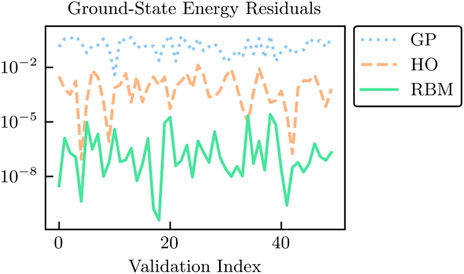
FIGURE 6. Absolute residuals in the energy (in MeV) at the 50 validation points for the RBM, HO, and GP emulators. The validation points are chosen randomly from a uniform distribution within the same range as the training points. See the main text for details.

FIGURE 7

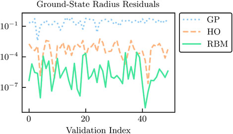
FIGURE 7. Similar to Figure 6 but for the root-mean-squared radius $\sqrt{⟨R^2⟩}$ and in units of fm.

The HO emulator performs better than the GP emulator, but it was not “trained” per se, it was merely given a basis of the lowest six HO wave functions as a trial basis, from which a reduced-order model was derived. However, the HO emulator can still outperform the GP emulator because it takes advantage of the structure of the high-fidelity system: it is aware that the problem to be solved is an eigenvalue problem, for this is built into the emulator itself. This feature permits a single HO emulator to emulate the wave function, energy, and radius simultaneously.

Coming in first in the comparison of the emulators’ performances is the RBM emulator, which typically results in higher accuracies than the HO and GP emulators by multiple orders of magnitude. The RBM emulator combines the best ideas from the other emulators. Like the GP, the RBM emulator uses evaluations of the eigenvalue problem as training data. However, its “training data” are curves (i.e., the wave functions) rather than scalars (e.g., eigen-energies), like the GP is trained upon. Like the HO emulator, the RBM emulator takes advantage of the structure of the system when projecting the high-fidelity system to create the reduced-order model. With these strengths, the RBM emulator is highly effective in emulating bound-state systems, even with only a few snapshots and far from the support of the snapshots (see Figures 1 and 2 in Ref. [25]). As we will see in Section 4, many of these strengths carry over to systems of differential equations.

3 Model reduction

In this Section, we provide a more general discussion of variational principles and the Galerkin method as the foundations for constructing highly efficient emulators for nuclear physics (see also Ref. [18]). The general methods discussed here will be used as a springboard to develop emulators for the specific case of scattering systems in Section 4.

We consider (time-independent) differential equations that depend on the parameter vector θ and aim to find the solution ξ of

$D\left(\xi ;\mathit{\theta }\right)=0\text{in\hspace{0.17em}}\mathrm{\Omega },(\mathrm{17a})$

$B\left(\xi ;\mathit{\theta }\right)=0\text{on\hspace{0.17em}}\mathrm{\Gamma },(\mathrm{17b})$

where {D, B} are differential operators and Ω is the domain with boundary Γ. See Ref. [18] for illustrative examples. Here, we use the generic function ξ because different choices of ξ will be made in Section 4. In what follows, we will discuss two related methods for constructing emulators from Eq. 17, which states the physics problem in a strong form (i.e., Eq. 17 holds for each point in the domain and on the boundary). The first begins by finding a variational principle whose stationary solution implies Eq. 17. The second instead constructs the corresponding weak form of Eq. 17.

3.1 Variational principles

Variational principles (VPs) have a long history in physics and play a central role in a wide range of applications; e.g., for deriving equations of motion using stationary-action principles and Euler–Lagrange equations in classical mechanics (see, e.g., Ref. [81] for a historical overview). Here, we use VPs as an alternate way of solving the differential Eq. 17.

Variational principles are based on scalar functionals of the form

$\mathcal{S}[\xi ]={\int }_{\mathrm{\Omega }}\mathrm{d}\mathrm{\Omega }F\left[\xi \right]+{\int }_{\mathrm{\Gamma }}\mathrm{d}\mathrm{\Gamma }G\left[\xi \right],(18)$

where F and G are differential operators. Many differential Eq. 17 can be solved by finding stationary solutions of a corresponding functional Eq. 18; i.e., the solution ξ_⋆ that leads to $\delta \mathcal{S}[{\xi }_{\star }]=0$.

However, VPs can also lead straightforwardly to a reduced-order model. This follows from the following trial ansatz

$|\tilde{\xi }\rangle \equiv \sum _{i=1}^{n_b}{\beta }_i|{\xi }_i\rangle =X\vec{\beta },(\mathrm{19a})$

$X\equiv \left[\begin{array}{cccc}\hfill |{\xi }_1\rangle \hfill & \hfill |{\xi }_2\rangle \hfill & \hfill \cdots \hfill & \hfill |{\xi }_{n_b}\rangle \hfill \end{array}\right],(\mathrm{19b})$

with the to-be-determined coefficients vector $\vec{\beta }$. Rather than stipulate that $\delta \mathcal{S}=0$ for any arbitrary variation δξ, we instead extract the optimal coefficients, ${\vec{\beta }}_{\star }$, as those for which $\mathcal{S}$ is stationary under variations in $\vec{\beta }$:⁶

$\delta \mathcal{S}=\sum _{i=1}^{n_b}\frac{\partial \mathcal{S}}{\partial {\beta }_i}\delta {\beta }_i=0.(20)$

The general case would involve a numerical search for the solution to Eq. 20 but if $\mathcal{S}$ is quadratic in ξ, as are all the examples considered here, then the solution can be determined exactly. In this case, $\mathcal{S}$ can be written as

$\mathcal{S}[\vec{\beta }]=\frac{1}{2}{\vec{\beta }}^{⊺}A\vec{\beta }+\vec{b}\cdot \vec{\beta }+c(21)$

for some matrix A, vector $\vec{b}$, and scalar c. Symmetrizing the quadratic portion—if it is not already symmetric—by rewriting A ← (A + A^⊺)/2 can be desirable for numerical purposes. It then follows that the optimal coefficients, ${\vec{\beta }}_{\star }$ are those for which

$\delta \mathcal{S}=A{\vec{\beta }}_{\star }+\vec{b}=0,(22)$

which can be solved for ${\vec{\beta }}_{\star }$ using standard linear algebra methods. Solving for ${\vec{\beta }}_{\star }$ occurs only in a space of size n_b, the number of basis elements ${\{{\xi }_i\}}_{i=1}^{n_b}$, rather than in the much larger space of ξ itself. Therefore, as long as ${\{{\xi }_i\}}_{i=1}^{n_b}$ approximately spans the space in which ξ lives, the trial function constructed by Eqs. 19a and 22 will be both a fast and accurate emulator of ξ.

Similar to the discussion in Section 2.1, the matrix A in Eq. 22 may be ill-conditioned and require regularization. A nugget ν ≪ 1 can be added to the diagonal elements of A to help stabilize the solution for ${\vec{\beta }}_{\star }$ [54, 55].

3.2 Galerkin emulators

The Galerkin approach, also more broadly called the “method of weighted residuals,” relies on the weak formulation of the differential Eq. 17. To obtain the weak form, the differential equation and boundary condition (in Eq. 17) are left-multiplied by arbitrary test functions ζ and $\bar{\zeta }$ and integrated over the domain and boundary, respectively, and then their sum is set to zero:

${\int }_{\mathrm{\Omega }}\mathrm{d}\mathrm{\Omega }\zeta D\left(\xi \right)+{\int }_{\mathrm{\Gamma }}\mathrm{d}\mathrm{\Gamma }\bar{\zeta }B\left(\xi \right)=0.(23)$

If Eq. 23 holds for all ζ and $\bar{\zeta }$, then Eq. 17) must be satisfied as well. The form of Eq. 23 is often rewritten using integration by parts to reduce the order of derivatives and simplify the solution. Importantly, the weak form has the integral form needed for our emulator application. The weak form and its Galerkin projection are used extensively, e.g., in the finite element method; see Refs. [82–84] for an in-depth study and examples. For a discussion of the convergence properties of the Galerkin method, its relation to abstract variational problems, and other salient mathematical details, see Refs. [64, 85–87]. Here, we follow the introduction of Galerkin methods as provided in Ref. [82].

Starting with the weak form, we can construct an emulator that avoids the need for an explicit variational principle. It begins by first noting that substituting our trial function Eq. 4 into D(ξ) and B(ξ) will not, in general, satisfy Eq. 17 regardless of the choice of $\vec{\beta }$. Therefore, there will be some residual, and the goal is to find the ${\vec{\beta }}_{\star }$ which minimizes that residual across a range of test functions ζ and $\bar{\zeta }$. This system would be over-determined in the case of truly arbitrary test functions, so instead, we propose the test bases

$|\zeta \rangle =\sum _{i=1}^{n_b}\delta {\beta }_i|{\zeta }_i\rangle ,|\bar{\zeta }\rangle =\sum _{i=1}^{n_b}\delta {\beta }_i|{\bar{\zeta }}_i\rangle ,(24)$

where δβ_i are arbitrary parameters, not related to the β_i in Eq. 19a. The δβ_i will play the same role as those in Eq. 20, namely as a bookkeeping method for determining the set of equations that are equivalently zero. By enforcing that the residuals against these test functions vanish for arbitrary δβ_i, the bracketed expression in

$\delta {\beta }_i\left[{\int }_{\mathrm{\Omega }}\mathrm{d}\mathrm{\Omega }{\zeta }_{i}D\left(X{\vec{\beta }}_{\star }\right)+{\int }_{\mathrm{\Gamma }}\mathrm{d}\mathrm{\Gamma }{\bar{\zeta }}_{i}B\left(X{\vec{\beta }}_{\star }\right)\right]=0,(25)$

is zero for all i ∈ [1, n_b], from which the optimal ${\vec{\beta }}_{\star }$ are extracted. Because this approximately satisfies the weak formulation, we have found an approximate solution to Equation (17).

In a variety of cases [82], the subspace $\mathcal{Z}$ spanned by the test function basis is chosen to coincide with the subspace $\mathcal{X}$ spanned by the trial function basis X; i.e., $\mathcal{Z}=\mathcal{X}$. This particular choice is known as the Galerkin method, but it is sometimes further specified as the Ritz–Galerkin or Bubnov–Galerkin methods. The Galerkin method is more general than the variational methods described in Section 3.1 because the test space need not be equivalent to the trial space (i.e., $\mathcal{Z}\ne \mathcal{X}$). In these cases, the approach is described as the Petrov–Galerkin method [82]; this can result in more efficient emulators for some differential equations (84).

4 Scattering emulators

In this Section, we describe various reduced-basis emulators one could construct for quantum scattering systems. Throughout, we note how the variational principles used to construct emulators in recent works are related [30–33, 88]. We also describe how each of the results from VPs could instead be derived from Galerkin projections.

For scattering problems, the Equation 1 is no longer an eigenvalue problem. The task is to solve the differential equation for the wave function at a given energy E rather than searching for discrete energies with normalizable wave functions. Differential equations are well studied in the field of MOR, where parametric reduced-order models have been constructed with great success across a multitude of fields [44, 89]. This is a relatively mature field whose formal results are quite extensive. For example, UQ for the RBM has been well studied, along with the development of effective algorithms for choosing the best training points [64, 76, 77, 90].

One can formulate the Schrödinger equation in multiple ways, including any flavor of Lippmann-Schwinger (LS) integral equation (which builds in boundary conditions) or as a differential equation in either homogeneous or inhomogeneous form. This freedom, along with the freedom of trial and test bases for the Galerkin projection, leads to multiple alternative emulators that one could construct for quantum scattering systems. For simplicity, we restrict our discussion to two-body scattering for Hermitian Hamiltonians. (See, however, Section 4.6.2 for an extension to higher-body systems.) As a concise reference, we provide Table 1 to show the connections between the fundamental differential or integral equations, variational principles, and Galerkin projections. This section thus provides multiple distinct examples of using Galerkin projections to create emulators, which may prove useful to newcomers wishing to apply model reduction to their own systems, and ends with an example for an emulator applied to a separable potential.

TABLE 1

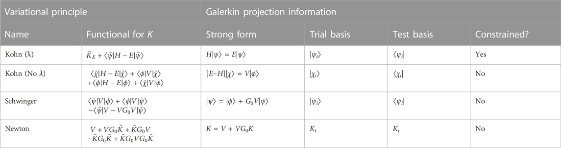
TABLE 1.  Description of common variational principles (VPs) in quantum scattering, and how to relate them to a Galerkin projection. The quantities are defined as the free wave function |ϕ⟩, the full wave function |ψ⟩, the scattered wave function |χ⟩, and the reactance matrix K along with its on-shell form K_E. Tildes denote trial quantities. The expressions for the Newton VP are written in operator rather than scalar form; any matrix element can be made individually stationary (see Section 4.4 for details). To compute the weak form of the Schwinger and Newton VPs, one must first left multiply by V(θ) and G₀, respectively, before orthogonalizing against the test basis. The rightmost column specifies whether a constraint for the trial wave function has to be imposed (e.g., using a Lagrange multiplier λ).

4.1 Constrained Kohn emulators

The Kohn variational principle (KVP) [91, 92] is one of the most well-known VPs for quantum scattering systems. Here we focus on the KVP flavor that relates a trial wave function to the reactance matrix K. However, alternative flavors exist for other matrices such at T^± and S (see Section 4.6). Analogously to the Ritz VP for bound states, the KVP then allows us to guess effective wave functions by finding those that make the KVP stationary. This Section will discuss a style of KVP emulator that relies on the homogeneous Schrödinger equation, which requires a normalization constraint during emulation; an alternative style without such a constraint will be discussed in Section 4.2.

We start with a rescaled version of the KVP discussed in Ref. [30]:

$\mathcal{K}\left[\tilde{\psi }\right]={\tilde{K}}_E+⟨\tilde{\psi }|H-E|\tilde{\psi }⟩,(26)$

where $|\tilde{\psi }\rangle$ is the trial wave function (denoted by $|\tilde{\xi }\rangle$ in Section 3) and ${\tilde{K}}_E\equiv {\sum }_i{\beta }_i{K}_{E,i}$ the associated on-shell trial K matrix with on-shell energy E = q²/2μ. This flavor of KVP applies when ψ satisfies the asymptotic normalization condition in position space

${\psi }_{\ell }\left(r\right)\underset{r\to \infty }{\to }{j}_{\ell }\left(qr\right)+n_{\ell }\left(qr\right)\tan {\delta }_{\ell },(27)$

where ϕ(r) = j_ℓ(qr) is the (regular) free-space wave function, and j_ℓ(qr) and n_ℓ(qr) are spherical Bessel and Neumann functions, respectively. ⁷ Note that we define the on-shell K_E matrix as

$K_E=-\frac{\tan {\delta }_{\ell }}{2\mu q},(28)$

which differs from the convention in Ref. [30]. The KVP is stationary about exact solutions ψ, such that $\mathcal{K}[\psi +\delta \psi ]=K_E+\mathcal{O}{(\delta K)}^2$.

Eq. 26 can be cast into the form of the generic functional (Eq. 18) by noting that, in position space,

$\begin{array}{ll}\hfill {\int }_{\mathrm{\Gamma }}\mathrm{d}\mathrm{\Gamma }G\left[\tilde{\psi }\right]\to {\left.G\left[\tilde{\psi }\right]\right|}_{r=0}^{\infty }& \equiv {\left.\frac{W\left(r\varphi ,r\tilde{\psi };r\right)}{2\mu }\right|}_{r=0}^{\infty }\hfill \\ \hfill & ={\tilde{K}}_E,\hfill \end{array}(29)$

which has defined the surface functional G in Eq. 18 and where we have used the Wronskian

$W\left(\varphi ,\psi ;r\right)\equiv \varphi \left(r\right){\psi }^{\prime }\left(r\right)-{\varphi }^{\prime }\left(r\right)\psi \left(r\right).(30)$

Both rϕ(r) and $r\tilde{\psi }(r)$ vanish at r = 0 so only the limit of r → ∞ contributes, from which we can use Eq. 27 when evaluating Eq. 29.

Because the Schrödinger equation is a linear, homogeneous differential equation, the normalization of rψ(r) is proportional to its derivative at, say, r = 0. Therefore, a constraint on the normalization of ψ is equivalent to a boundary condition on ψ′. However, to satisfy this boundary condition we must include a constraint on Eq. 26 if we are to ensure that the trial function $\tilde{\psi }$ continues to satisfy the normalization condition of Eq. 27. If we assume that each snapshot ψ_i satisfies Eq. 27, then

${\tilde{\psi }}_{\ell }\left(r\right)=\left[\sum _i{\beta }_i\right]j_{\ell }\left(qr\right)+n_{\ell }\left(qr\right)\sum _i{\beta }_i\tan {\delta }_{\ell ,i},(31)$

whose first term implies that we must impose the constraint ∑_iβ_i = 1.

We are now in a position to find the $\vec{\beta }$ that make Eq. 26 stationary. If we insert the definition of $\tilde{\psi }$ and $\tilde{K}$ into Eq. 26, along with the Lagrange multiplier, we have (with repeated indices indicating summations)

$\mathcal{K}\left[\vec{\beta }\right]={\beta }_i{K}_{E,i}+\frac{1}{2}{\beta }_i\mathrm{\Delta }{\tilde{U}}_{ij}{\beta }_j+\lambda \left[\sum _i{\beta }_i-1\right],(32)$

where we define V_i = V(θ_i) and

$\begin{array}{ll}\hfill \mathrm{\Delta }{\tilde{U}}_{ij}& \equiv ⟨{\psi }_i|H-E|{\psi }_j⟩+\left(i\leftrightarrow j\right)\hfill \\ \hfill & =⟨{\psi }_i|V\left(\mathit{\theta }\right)-V_j|{\psi }_j⟩+\left(i\leftrightarrow j\right).\hfill \end{array}(33)$

In the second line we have used that the |ψ_j⟩ are eigenstates with the corresponding V_j. If V(θ) is affine in θ, then $\mathrm{\Delta }\tilde{U}$ can be projected once in the emulator’s offline stage, and reconstructed quickly during the online stage.

Now we can follow the steps outlined in Section 3.1 to determine ${\vec{\beta }}_{\star }$. Taking the gradient of Eq. 32 with respect to $\vec{\beta }$ and setting it equal to 0 yields

${\vec{K}}_E+\mathrm{\Delta }\tilde{U}{\vec{\beta }}_{\star }+{\lambda }_{\star }=0,(34)$

where ${\vec{K}}_E$ are the n_b on-shell K-matrices used to train the emulator, and ${\vec{\beta }}_{\star }$ are the optimal coefficients of the trial wave function. The gradient with respect to λ simply returns the constraint. This system can be solved via the system of equations

$\left[\begin{array}{cc}\hfill \mathrm{\Delta }\tilde{U}\hfill & \hfill \vec{1}\hfill \\ \hfill \vec{1}{}^{⊺}\hfill & \hfill 0\hfill \end{array}\right]\left[\begin{array}{c}\hfill {\vec{\beta }}_{\star }\hfill \\ \hfill {\lambda }_{\star }\hfill \end{array}\right]=\left[\begin{array}{c}\hfill -{\vec{K}}_E\hfill \\ \hfill 1\hfill \end{array}\right],(35)$

where $\vec{1}$ is an n_b × 1 vector of ones. If the n_b number of basis functions is much smaller than the size of ψ, then Eq. 35 can be a highly computationally efficient emulator for scattering systems and requires little computer memory to store. The on-shell K matrix can then be emulated via

$K_E\approx \mathcal{K}\left[{\vec{\beta }}_{\star }\right]={\vec{\beta }}_{\star }\cdot {\vec{K}}_E+\frac{1}{2}{\vec{\beta }}_{\star }^{⊺}\mathrm{\Delta }\tilde{U}{\vec{\beta }}_{\star },(36)$

whose operations all occur quickly in the size-n_b space during the online stage.

The derivation above followed closely that of Refs [30, 93], but one could instead arrive at exactly Eq. 35 from a Galerkin projection [43]. Rather than begin with the VP, we start here with (the strong form of) the homogeneous Schrödinger equation, i.e., H(θ)|ψ⟩ = E|ψ⟩. To construct the weak form, we multiply with a test function |ζ⟩ and assert that the residual vanishes:

$⟨\zeta |H-E|\psi ⟩=0,\forall |\zeta \rangle .(37)$

To make explicit the boundary conditions, we make use of the relation

$\begin{array}{ll}\hfill 0& =⟨\zeta |H-E|\psi ⟩\hfill \\ \hfill & =⟨\zeta |\stackrel{⃖}{H}-E|\psi ⟩-{\left.\frac{W\left(r\zeta ,r\psi ;r\right)}{2\mu }\right|}_{r=0}^{\infty },\hfill \end{array}(38)$

where we have again used the Wronskian from Eq. 30, and assigned $\stackrel{⃖}{H}$ as the operator acting, after integration by parts, on ⟨ζ| instead of |ψ⟩. By adding Eqs. 38 and 37, we have

$⟨\zeta |H-E|\psi ⟩+⟨\zeta |\stackrel{⃖}{H}-E|\psi ⟩={\left.\frac{W\left(r\zeta ,r\psi ;r\right)}{2\mu }\right|}_{r=0}^{\infty }.(39)$

This is the weak form of the homogeneous Schrödinger equation that we will use to construct the emulator, although the asymptotic normalization condition Eq. 27 still needs to be enforced. This will be imposed via a Lagrange multiplier after inserting our trial basis.

Now that we have a weak form, the next step to construct the reduced-order model equations is to define our trial and test bases to project the weak form into the finite space of these bases. To align with the Kohn emulator from the variational argument above, we choose the trial and test basis to be identical as snapshots ψ_i. Then we can evaluate

${\left.\frac{W\left(r{\psi }_i,r{\psi }_j;r\right)}{2\mu }\right|}_{r=0}^{\infty }=K_j-K_i(40)$

and thus, it follows after including the Lagrange multiplier that

$\lambda +\left[⟨{\psi }_i|H-E|{\psi }_j⟩+⟨{\psi }_i|\stackrel{⃖}{H}-E|{\psi }_j⟩\right]{\beta }_j=\sum _j{\beta }_j{K}_j-K_i\sum _j{\beta }_j.(41)$

The sum in the rightmost term can be evaluated using the constraint ∑_j β_j = 1, and we can make the redefinition λ′ ≡ λ−∑_j β_j K_j without impacting the solution because this term does not depend on i. Thus, we have

${\lambda }^{\prime }+{\vec{K}}_E+\mathrm{\Delta }\tilde{U}{\vec{\beta }}_{\star }=0,(42)$

which is exactly Eq. 34 found by making the KVP stationary. This simplification can be understood by noting that if $\{{\vec{\beta }}_{\star },{\lambda }_{\star }\}$ satisfy Eq. 41, then we know that $\{{\vec{\beta }}_{\star },{\lambda }_{\star }^{\prime }\}$ is the unique solution to Eq. 42. Therefore, we can solve Eq. 42 to obtain ${\vec{\beta }}_{\star }$ rather than Eq. 41. In conclusion, using the Galerkin projection of the homogeneous Schrödinger equation with trial and test bases of ψ_i, we were able to obtain the same coefficients as the KVP in Eq. 35, which yield the same on-shell K matrix when used in Eq. 36.

4.2 Unconstrained Kohn emulators

The Kohn emulators from Section 4.1 start with the homogeneous Schrödinger equation, which does not enforce any specific normalization of the wave function; hence this requirement needs to be enforced at the time of emulation. This effectively takes the n_b degrees of freedom {ψ_i}—which were potentially costly to obtain—and reduces the degrees of freedom to n_b−1. However, one can instead build in the normalization from the very start, thus removing the need to constrain our basis via ${\sum }_{j=1}^{n_b}{\beta }_j=1$ during emulation. The unconstrained emulator is fundamentally different from any approach that constrains the coefficients (e.g., explicit substitution of ${\beta }_1=1-{\sum }_{j=2}^{n_b}{\beta }_j$), regardless of if a Lagrange multiplier is explicitly used as in Section 4.1. This is the topic of the current section.

The full wave function |ψ⟩ can be written as the sum of the free wave function |ϕ⟩ and the scattered wave |χ⟩, that is, |ψ⟩ = |ϕ⟩ + |χ⟩. Thus, we can rewrite the KVP as

$\begin{array}{ll}\hfill \mathcal{K}& =K+⟨\psi |\left[H-E\right]|\psi ⟩\hfill \\ \hfill & =K+⟨\chi |\left[H-E\right]|\chi ⟩+⟨\varphi |\left[H-E\right]|\chi ⟩\hfill \\ \hfill & +⟨\varphi |\left[H-E\right]|\varphi ⟩+⟨\chi |\left[H-E\right]|\varphi ⟩\hfill \\ \hfill & =⟨\chi |\left[H-E\right]|\chi ⟩+⟨\varphi |V|\chi ⟩+⟨\varphi |\left[H-E\right]|\varphi ⟩+⟨\chi |V|\varphi ⟩,\hfill \end{array}(43)$

where we used (via integration by parts)

$⟨\varphi |\left[H-E\right]|\chi ⟩-⟨\varphi |\left[\stackrel{⃖}{H}-E\right]|\chi ⟩=-K.(44)$

We choose our trial function as $|\tilde{\chi }\rangle$, which always enforces the normalization condition $|\tilde{\psi }\rangle =|\varphi \rangle +|\tilde{\chi }\rangle$, and so no additional constraint needs to be included in the variational principle.

Now we can construct the set of linear equations that makes Eq. 43 stationary in $|\tilde{\chi }\rangle ={\sum }_i{\beta }_i|{\chi }_i\rangle$. By taking the gradient with respect to β_i, we find

$\mathrm{\Omega }{\vec{\beta }}_{\star }=\vec{\omega },(45)$

where

${\mathrm{\Omega }}_{ij}=⟨{\chi }_i|\left[E-H\right]|{\chi }_j⟩,(\mathrm{46a})$

${\omega }_i=⟨{\chi }_i|V|\varphi ⟩,(\mathrm{46b})$

which is the set of equations used to obtain ${\vec{\beta }}_{\star }$. The matrix elements Ω_ij can be evaluated with the help of

$\begin{array}{ll}\hfill \left[E-H\right]|{\chi }_j\rangle & =\left[E-H_j\right]|{\chi }_j\rangle +\left[V_j-V\right]|{\chi }_j\rangle \hfill \\ \hfill & =V_j|\varphi \rangle +\left[V_j-V\right]|{\chi }_j\rangle ,\hfill \end{array}(47)$

with H_j = H (θ_j) and V_j = V (θ_j).

An equivalent approach follows from a Galerkin orthogonalization procedure. We begin by writing the homogeneous Schrödinger equation in inhomogeneous form using |ψ⟩ = |ϕ⟩ + |χ⟩:

$\left[E-H\right]|\chi \rangle =V|\varphi \rangle .(48)$

We can construct the weak form by multiplying by a generic test function |ζ⟩, which yields

$⟨\zeta |E-H|\chi ⟩=⟨\zeta |V|\varphi ⟩.(49)$

Next, we insert the trial function $|\tilde{\chi }\rangle$ and choose the test basis of ${\{|{\chi }_i\rangle \}}_i$, which is the same as the trial basis. This yields a reduced weak form that is identical to Eq. 45.

We have shown that the coefficients ${\vec{\beta }}_{\star }$ found via the appropriate Galerkin procedure aligns exactly with the KVP. However, we can go one step further and in fact derive an estimate for the K matrix that is equivalent to $\mathcal{K}[{\vec{\beta }}_{\star }]$. By inserting the optimal coefficients into K|ϕ⟩ = V|ψ⟩,

$\begin{array}{ll}\hfill ⟨{\varphi }^{\prime }|K|\varphi ⟩& \approx ⟨{\varphi }^{\prime }|V|\varphi ⟩+⟨{\varphi }^{\prime }|V|\tilde{\chi }⟩\hfill \\ \hfill & =⟨{\varphi }^{\prime }|V|\varphi ⟩+\sum _{ij}⟨{\varphi }^{\prime }|V|{\chi }_i⟩\left[{\left({\mathrm{\Omega }}^{-1}\right)}_{ij}⟨{\chi }_j|V|\varphi ⟩\right],\hfill \end{array}(50)$

with the factors in brackets equating to β_i using Eq. 45. The equivalence to the KVP is demonstrated in Refs. [94, 95].

4.3 Schwinger emulators

The Schwinger variational principle (SVP) is given by [94].

$\mathcal{K}\left[\tilde{\psi }\right]=⟨\tilde{\psi }|V|\varphi ⟩+⟨\varphi |V|\tilde{\psi }⟩-⟨\tilde{\psi }|V-V{G}_{0}V|\tilde{\psi }⟩,(51)$

where G₀ is the Green’s operator. This too has the stationary property $\mathcal{K}[\psi +\delta \psi ]=K+\mathcal{O}{(\delta K)}^2$ when ψ is a wave function satisfying the LS equation. Following the MOR philosophy and inserting a trial function $\tilde{\psi }$, the stationary condition becomes

$W{\vec{\beta }}_{\star }=\vec{w},(52)$

where

$W_{ij}=⟨{\psi }_i|V-V{G}_{0}V|{\psi }_j⟩(\mathrm{53a})$

$w_i=⟨{\psi }_i|V|\varphi ⟩,(\mathrm{53b})$

for all i ∈ [1, …, n_b].

The system of Eq. 52 can also be determined by a Galerkin projection procedure. In this case, we start with the LS equation for wave functions,

$|\psi \rangle =|\varphi \rangle +G_{0}V|\psi \rangle ,(54)$

and create a weak form by left-multiplying by V(θ) along with the test function |ζ⟩:

$⟨\zeta |V|\psi ⟩=⟨\zeta |V|\varphi ⟩+⟨\zeta |V{G}_{0}V|\psi ⟩.(55)$

The weak form can then be converted to its discrete form by setting $\psi \to \tilde{\psi }$ and enforcing orthogonality against |ζ_i⟩ = |ψ_i⟩ for i ∈ [1, …, n_b]. ⁸ This yields then Eq. 52, and so the coefficients found by making Eq. 51 stationary are indeed identical to those found via the Galerkin procedure for Eq. 54.

Using the emulation of ψ, which is calculated by inserting the optimal coefficients obtained from Eq. 52 into the definition of $\tilde{\psi }$, we can get the associated K through

$\begin{array}{ll}\hfill ⟨{\varphi }^{\prime }|K|\varphi ⟩& =⟨{\varphi }^{\prime }|V|\psi ⟩\hfill \\ \hfill & \approx ⟨{\varphi }^{\prime }|V|\tilde{\psi }⟩\hfill \\ \hfill & =\sum _{ij}⟨{\varphi }^{\prime }|V|{\psi }_i⟩{\left(W^{-1}\right)}_{ij}⟨{\psi }_j|V|\varphi ⟩.\hfill \end{array}(56)$

This Equation is exactly the solution for K found via the LS equation while assuming a finite-rank approximation for V:

$V^f=\sum _{ij}V|{\psi }_i\rangle {\mathrm{\Lambda }}_{ij}\langle {\psi }_j|V,(57)$

where

${\left({\mathrm{\Lambda }}^{-1}\right)}_{ij}=⟨{\psi }_i|V|{\psi }_j⟩.(58)$

It is known that the SVP yields a K matrix that is equivalent to that found via a finite-rank approximation to V [94, 95], which shows that the Galerkin projection described in this Section is identical to the SVP.

4.4 Newton emulators

The Newton variational principle (NVP) for the K matrix is given by [31, 96].

$\mathcal{K}\left[\tilde{K}\right]=V+V{G}_0\tilde{K}+\tilde{K}{G}_{0}V-\tilde{K}{G}_0\tilde{K}+\tilde{K}{G}_{0}V{G}_0\tilde{K},(59)$

where $\tilde{K}$ is a trial matrix. If desired, one could instead emulate T^(±) by imposing the associated boundary conditions on G₀. Here it is assumed that we have chosen an on-shell energy E, which will remain implicit throughout. A separate emulator can be constructed for each choice of E. The functional Eq. 59 is stationary about exact solutions of the LS equation, i.e., $\mathcal{K}[K+\delta K]=K+{(\delta K)}^2$. If we write the trial matrix as a linear combination of exact snapshots

$\tilde{K}=\sum _{i=1}^{n_b}{\beta }_i{K}_i,(60)$

then we can construct an emulator of the K matrix in the spirit of the RBM.

Unlike some of the VPs discussed so far, the NVP is written here in operator form, without yet projecting it into a basis. This gives us the freedom to assert that any component $⟨{\varphi }^{\prime }|\mathcal{K}|\varphi ⟩$ constructed from Eq. 59 is stationary, which yields an emulator for ⟨ϕ′|K|ϕ⟩. For example, one could choose |ϕ⟩ to be a plane-wave partial-wave basis |kℓm⟩ with momentum k and angular momentum quanta (l, m), or one could keep the angular dependence explicit via |ϕ⟩ = |k⟩ in a single-particle basis. Coupled channels could be emulated by choosing the angular momentum quanta differently between |ϕ′⟩ and |ϕ⟩. In fact, the NVP does not even require |ϕ⟩ and |ϕ′⟩ to be free-space states; one can impose stationarity of Eq. 59 between any two states due to its operator form. Note that the independent coefficients $\vec{\beta }$ are found for each choice of |ϕ′⟩ and |ϕ⟩. Thus, in the case of coupled partial waves, for example, each channel is emulated independently. To compute phase shifts, we must emulate K at the on-shell energy E = q²/2μ and thus, k = k′ = q for |ϕ⟩ = |kℓm⟩ and ⟨ϕ′| = ⟨k′ℓ′m′|.

Expressed in the chosen basis, simplifying the functional Eq. 59 after inserting Eq. 60 yields [31]

$⟨{\varphi }^{\prime }|\mathcal{K}\left(\mathit{\theta },\vec{\beta }\right)|\varphi ⟩=⟨{\varphi }^{\prime }|V\left(\mathit{\theta }\right)|\varphi ⟩+{\vec{\beta }}^{⊺}\vec{m}\left(\mathit{\theta }\right)-\frac{1}{2}{\vec{\beta }}^{⊺}M\left(\mathit{\theta }\right)\vec{\beta },(61)$

with

$m_i\left(\mathit{\theta }\right)=⟨{\varphi }^{\prime }|\left[K_i{G}_{0}V\left(\mathit{\theta }\right)+V\left(\mathit{\theta }\right)G_0{K}_i\right]|\varphi ⟩,(\mathrm{62a})$

$M_{ij}\left(\mathit{\theta }\right)=⟨{\varphi }^{\prime }|\left[K_i{G}_0{K}_j-K_i{G}_{0}V\left(\mathit{\theta }\right)G_0{K}_j\right]|\varphi ⟩+\left(i\leftrightarrow j\right).(\mathrm{62b})$

If the potential V(θ) has an affine parameter dependence, $\vec{m}$ and M can be efficiently constructed by linear combinations of matrices pre-computed during the emulator’s offline stage, resulting in substantial improvements in CPU time, e.g., for chiral interactions.

By imposing the stationary condition $\partial \mathcal{K}/\partial \vec{\beta }=0$, one then finds ${\vec{\beta }}_{\star }(\mathit{\theta })$ such that $M{\vec{\beta }}_{\star }=\vec{m}$. Given that the optimal ${\vec{\beta }}_{\star }(\mathit{\theta })$ yields a trial matrix Eq. 60 with an error δK, one can insert ${\vec{\beta }}_{\star }$ in Eq. 61 to obtain an error (δK)². The resulting emulator ${\mathcal{K}}_{\star }(\mathit{\theta })\equiv \mathcal{K}(\mathit{\theta },{\vec{\beta }}_{\star })$ is then [31]

$⟨{\varphi }^{\prime }|K|\varphi ⟩\approx ⟨{\varphi }^{\prime }|\mathcal{K}|\varphi ⟩=⟨{\varphi }^{\prime }|V|\varphi ⟩+\frac{1}{2}{\vec{m}}^{⊺}{M}^{-1}\vec{m}.(63)$

Reference [31] studied several applications of the emulator Eq. 63 to short-range potentials with and without the Coulomb interaction and partial-wave coupling. They demonstrated that the NVP emulator has remarkable extrapolation capabilities (see Figure 2 in Ref. [31]) and can quickly reproduce high-fidelity calculations of neutron-proton cross sections based on modern chiral interactions with negligible error.

We now repeat the derivation for the NVP emulator, but instead from the perspective of a Galerkin projection. Here, we will focus on the case where ⟨ϕ′| = ⟨ϕ|. We start with the LS equation

$K=V+V{G}_{0}K,(64)$

which, in this context, constitutes the strong form of the integral equation. Although Eq. 64 is written in terms of abstract operators, it can be turned into a vector equation in a specific representation after right-multiplying by |ϕ⟩. To derive the weak form we left-multiply by G₀ and a test function ⟨ζ|:

$⟨\zeta |G_{0}K-G_{0}V{G}_{0}K|\varphi ⟩=⟨\zeta |G_{0}V|\varphi ⟩.(65)$

The trial function in this case is K|ϕ⟩, which can be expanded in a discrete (snapshot) basis using Eq. 60. We further employ the Galerkin prescription, where the test basis is equivalent to the trial basis, making ⟨ζ_i| = ⟨ϕ|K_i. With these assumptions, the reduced weak form becomes

$M{\vec{\beta }}_{\star }=\vec{m},(66)$

with M and $\vec{m}$ defined in Equation (62), again with ⟨ϕ′| = ⟨ϕ|. Thus, we find the same ${\vec{\beta }}_{\star }$ using either the NVP or the Galerkin projection.

Given the optimal coefficients ${\vec{\beta }}_{\star }$, the emulator can be derived by substituting $\tilde{K}$ into the right-hand side of Eq. 64:

$\begin{array}{ll}\hfill ⟨\varphi |K|\varphi ⟩& \approx ⟨\varphi |V|\varphi ⟩+⟨\varphi |V{G}_0\tilde{K}|\varphi ⟩\hfill \\ \hfill & =⟨\varphi |V|\varphi ⟩+\frac{1}{2}{\vec{m}}^{⊺}{M}^{-1}\vec{m},\hfill \end{array}(67)$

which is equivalent to Eq. 63 under the assumption that ⟨ϕ′| = ⟨ϕ|. Therefore, both the NVP and Galerkin projection lead to identical emulators for the K matrix.

4.5 Origin emulators

The scattering emulators discussed so far are best known as VPs but are equivalent to various types of Galerkin projections of the Schrödinger or LS equation (see Table 1). However, other types of emulators can be constructed via Galerkin projections, even if they do not necessarily correspond to any well-known VP.

Starting from the Schrödinger equation—a second-order differential equation—we must impose two boundary conditions. The first is that rψ(r) vanishes at r = 0; this constraint has been automatically satisfied by our choice of trial bases in all VPs considered above. But the second constraint is yet to be chosen. In the KVP, for example, the second constraint was obtained via the normalization of rψ(r) as r → ∞, which, in the constrained KVP, led to a normalization constraint for the coefficients β_i. Because the Schrödinger equation is linear and homogeneous, this normalization condition is equivalent to imposing a constraint on the derivative of rψ(r), e.g., evaluated at the origin.

Thus, an alternative weak form for the Schrödinger equation could be constructed using only constraints at the origin. Let us construct a coordinate-space emulator with (rψ)′(0) = 1. Starting from the generic weak form (23), we obtain

$⟨\zeta |H-E|\psi ⟩+{\left.\bar{\zeta }\left[{\left(r\psi \right)}^{\prime }-1\right]\right|}_{r=0}=0,(68)$

where ζ and $\bar{\zeta }$ are the (independent) test functions in the domain and on the boundary, respectively, and the boundary condition is only evaluated at the origin. Here, we can make the Galerkin choice of (domain) test functions, where ⟨ζ| = ⟨ψ|, but make a Petrov-Galerkin choice for the boundary, with $\bar{\zeta }(0)=1$.

Thus, the discretized weak form, from which our emulator equations follow, is given by

$⟨{\psi }_i|H-E|{\psi }_j⟩{\beta }_j+\sum _j{\beta }_j-1=0,(69)$

where we have assumed that the trial basis is constructed such that each snapshot satisfies ${(r{\psi }_j)}^{\prime }(0)=1$.

As an example, we show the output of such an s-wave (ℓ = 0) emulator in Figure 8. Here, the potential is given by a sum of two Gaussians,

$V\left(r,\mathit{\theta }\right)={\theta }_1\exp \left(-{\kappa }_1{r}^2\right)+{\theta }_2\exp \left(-{\kappa }_2{r}^2\right),(70)$

with κ₁ = 0.5 and κ₂ = 1. The parameters to be varied are θ = {θ₁, θ₂}. The six training and one validation parameters are selected randomly from a uniform distribution in the range of [−5, 5]. To obtain the snapshots, the partial-wave decomposed radial Schrödinger equation for ℓ = 0 can be expressed as the system of coupled first-order differential equations,

$\left(\begin{array}{c}\hfill {y^{\prime }}_0(r)\hfill \\ \hfill {y^{\prime }}_1(r)\hfill \end{array}\right)=\left(\begin{array}{c}\hfill {(r\psi )}^{\prime }(r)\hfill \\ \hfill 2\mu \left[V(r;{\mathit{\theta }}_i)-E\right](r\psi )(r)\hfill \end{array}\right),(71)$

and numerically solved with Runge-Kutta methods. For more details on solving the radial Schrödinger equation and matching the solutions to the asymptotic boundary condition (27), see, e.g., Ref. [97]. As we can see from Figure 8, each training and emulated wave function has matching boundary conditions at the origin, and the discrepancy from the true wave function is less than 10^–3.

FIGURE 8

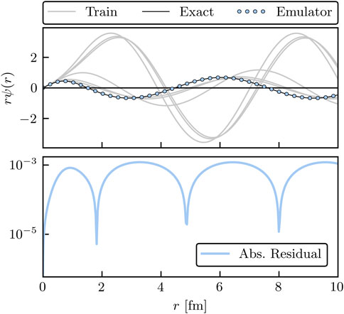
FIGURE 8. Results for the scattering emulator with origin boundary conditions in arbitrary units. Six basis functions are shown as gray lines, and the exact wave function as a black line. Each of the basis functions and the emulated wave function satisfy the constraints at the origin.

4.6 General Kohn variational principle

The KVP functional given in Eq. 26 can be extended to include arbitrary boundary conditions [32, 98]. For simplicity, let us consider short-range potentials V(θ) that have been partial-wave decomposed into an uncoupled channel with angular momentum ℓ. The general asymptotic form of the (coordinate-space) radial wave functions will be linear combinations of free-space solutions⁹

$\begin{array}{l}\hfill {\psi }_{\ell ,E}(r)\underset{r\to \infty }{\to }{\bar{\varphi }}_{\ell ,E}^{\left(\text{0}\right)}(r)+L_{\ell ,E}{\bar{\varphi }}_{\ell ,E}^{\left(1\right)}(r),\end{array}(72)$

where

$\left(\begin{array}{c}\hfill {\bar{\varphi }}_{\ell ,E}^{\left(\text{0}\right)}\left(r\right)\hfill \\ \hfill {\bar{\varphi }}_{\ell ,E}^{\left(1\right)}\left(r\right)\hfill \end{array}\right)={\mathcal{N}}^{-1}\left(\begin{array}{cc}\hfill u_{00}\hfill & \hfill u_{01}\hfill \\ \hfill u_{10}\hfill & \hfill u_{11}\hfill \end{array}\right)\left(\begin{array}{c}\hfill j_{\ell }\left(qr\right)\hfill \\ \hfill {\eta }_{\ell }\left(qr\right)\hfill \end{array}\right),(73)$

with $q=\sqrt{2\mu E}$ and an arbitrary normalization constant $\mathcal{N}\ne 0$. Here, L_ℓ,E is a generic scattering matrix that is determined by the boundary condition, as parametrized by the non-singular matrix u.

We now define $\mathcal{L}$ as a general functional for the generic L-matrix in Eq. 72 [32, 88, 98],

$\mathcal{L}[\tilde{\psi }]=L_{\ell ,E}+\frac{2\mu {\mathcal{N}}^2}{q\mathrm{d}\mathrm{e}\mathrm{t}\mathit{u}}\langle {\tilde{\psi }}_{\mathit{u}}|H-E|{\tilde{\psi }}_{\mathit{u}}\rangle .(74)$

Note that Eq. 74 is not restricted to coordinate space, e.g., it also holds for scattering in momentum space (see Ref. [88]). With Eq. 26, one can follow the process described in Section 4.1 to emulate any asympototic boundary condition. Obtaining an emulator prediction for different boundary conditions does not mean that Eq. 74 has to be solve multiple times. In fact, it only needs to be solved once and each term in the functional rescaled using the relations derived in Ref. [32]:

$\mathrm{\Delta }{\tilde{U}}^{\left({\mathit{u}}^{\prime }\right)}=C^{\prime -1}\left(L_i\right)C^{\prime -1}\left(L_j\right)\frac{\det \mathit{u}}{\det {\mathit{u}}^{\prime }}\mathrm{\Delta }{\tilde{U}}^{\left(\mathit{u}\right)},(75)$

$C^{\prime }\left(L\right)=\frac{\det \mathit{u}}{\det {\mathit{u}}^{\prime }}\frac{u_{11}^{\prime }-u_{10}^{\prime }K\left(L\right)}{u_{11}-u_{10}K\left(L\right)}.(76)$

The non-primed terms refer to the initial state and primed terms refer to the final state (explained below). The snapshots used to train the emulator in the offline stage are transformed using the Möbius (or linear fractional) transform

$L^{\prime }\left(L\right)=\frac{-u_{01}^{\prime }+u_{00}^{\prime }K\left(L\right)}{u_{11}^{\prime }-u_{10}^{\prime }K\left(L\right)}.(77)$

Let us consider solving Eq. 74 using the K-matrix boundary condition, but then wanting a prediction for the T-matrix. We would first rescale $\mathrm{\Delta }\tilde{U}$ using Eq. 75. Here, u and u′ would correspond to u_K and u_T, respectively, given by

${\mathit{u}}_K=\left[\begin{array}{cc}\hfill 1\hfill & \hfill 0\hfill \\ \hfill 0\hfill & \hfill 1\hfill \end{array}\right],{\mathit{u}}_T=\left[\begin{array}{cc}\hfill 1\hfill & \hfill 0\hfill \\ \hfill i\hfill & \hfill 1\hfill \end{array}\right].(78)$

Once $\mathrm{\Delta }{\tilde{U}}^{({\mathit{u}}^{\prime })}$ is calculated and the snapshots transformed from the K- to the T-matrix according to Eq. 77, we apply Eq. 35 to obtain the emulator prediction for the T-matrix. One can also inverse transform the new emulated solution back to its K-matrix equivalent by using

$K\left(L\right)=\frac{u_{01}+u_{11}L}{u_{00}+u_{10}L}.(79)$

Variational principles may not always provide a (unique) stationary approximation, causing the appearance of spurious singularities known as Kohn (or Schwartz) anomalies [32, 98, 101], which can render applications of VPs ineffective; especially for sampling of a model’s parameter space.¹⁰ The appearance of these anomalies depends on the parameters θ used to train the emulator in the offline stage, the scattering energy, and the evaluation set used in the online stage. However, Ref. [32] demonstrated that a KVP-based emulator that simultaneously emulates an array of KVPs with different boundary conditions can be used to systematically detect and remove these anomalies. The anomalies can be detected by assessing the (relative) consistency of the different emulated results for, e.g., the scattering S-matrix. The results that do not pass the consistency check are discarded and the remaining ones averaged to obtain an anomaly-free estimate of the S matrix (or any other matrix). If all possible consistency checks fail, one can change the basis size of the trial wave function iteratively, which typically shifts the locations of the Kohn anomalies in the parameter space in each iteration. The basic idea for removing Kohn anomalies is general and can be applied to other emulators, including the NVP-based emulator discussed in Section 4.4, as long as multiple scattering boundary conditions can be emulated independently and efficiently. Alternatively, one might also consider comparing the consistency of emulated results obtained from different VPs such as the ones summarized in Table 1.

4.6.1 Generalization to coupled systems

Following Ref. [88], let us now extend the generalized KVP in Section 4.6 to coupled systems, which could be coupled partial-wave or reaction channels. The stationary approximation to the high-fidelity L-matrix then reads

${\mathcal{L}}^{s{s}^{\prime }}={\beta }_i{L}_i^{s{s}^{\prime }}+\frac{1}{2}{\beta }_i\mathrm{\Delta }{\tilde{U}}_{ij}^{s{s}^{\prime }}{\beta }_j,(80)$

where

$\begin{array}{ll}\hfill \mathrm{\Delta }{\tilde{U}}_{ij}^{s{s}^{\prime }}& \equiv \frac{2\mu {\mathcal{N}}^2}{q\mathrm{d}\mathrm{e}\mathrm{t}\mathit{u}}\left[⟨{\psi }_i^s|H(\mathit{\theta })-E|{\psi }_j^{s^{\prime }}⟩\right.+\left.(i\leftrightarrow j)\right]\hfill \\ \hfill & =\frac{2\mu {\mathcal{N}}^2}{q\mathrm{d}\mathrm{e}\mathrm{t}\mathit{u}}\left[⟨{\psi }_i^s|V(\mathit{\theta })-V_j|{\psi }_j^{s^{\prime }}⟩\right.+\left.(i\leftrightarrow j)\right],\hfill \\ \hfill \end{array}(81)$

with s and s′ corresponding to the entrance and exit channels. The uncoupled case is retrieved by replacing ss′ → ℓ. Solving for $\vec{\beta }$ now proceeds as in Eq. 35 but for a specific choice of ss’ channels. Note that the coefficients $\vec{\beta }$ are to be determined independently for each ss′ pair.

The coefficients are independent because ${\mathcal{L}}^{s{s}^{\prime }}$ is independently stationary for each ss’ pair. This becomes apparent when considering how one would solve for the coefficients in the case where there are two uncoupled channels, where ss′ → ℓ in Eqs. 80 and 81. Here, each partial wave is completely independent of one another, and thus each VP and their corresponding coefficients $\vec{\beta }$ are independent of one another across values of ℓ. Without loss of generality, let the two channels be labeled as ℓ = 0 and ℓ = 1, and let ${\vec{\beta }}^{(0)}$ and ${\vec{\beta }}^{(1)}$ denote the independent sets of coefficients found by making each channel’s KVP stationary. Now consider adiabatically turning on a coupling between two partial waves: the coefficients ${\vec{\beta }}^{(0)}$ and ${\vec{\beta }}^{(1)}$ should remain nearly fixed to their previously uncoupled values, but now there is a new set of coefficients to determine, which one could label as ${\vec{\beta }}^{(01)}$. Thus, even in the coupled case, there are multiple independent sets of coefficients to determine: one for each pair of incoming and outgoing channels.

An alternative way to understand how the $\vec{\beta }$ enter in the coupled case is to instead start with the Schrödinger equation and enforce (Petrov-)Galerkin orthogonalization as in Section 4.1. For the diagonal channels, the test functions are chosen to have the same outgoing channel as the trial functions, making the procedure of standard Galerkin form. But for the off-diagonal channels, the test functions have a different outgoing channel (s) than the trial functions (s′). Because the basis of test functions differs from the basis of the trial function, this is instead a Petrov–Galerkin approach. The linear equations to be solved are exactly what one would obtain from enforcing stationarity in Eq. 80 for each ss′ independently. See Ref. [88] for more information on coupled channel emulation.

4.6.2 Generalizations to higher-body systems

The variational emulators for two-body scattering described so far can be generalized to higher-body scattering. In fact, the KVP, as a powerful method for solving scattering problems, has been applied in developing high-fidelity solvers (as opposed to a KVP-based emulator) for studying three- and four-nucleon systems (e.g., nucleon-deuteron elastic scattering below and above the deuteron break-up threshold) [103, 104].¹¹ It is then natural to combine the KVP with the variational emulation strategy to develop fast and accurate emulators beyond just two-body scattering.

Here, we follow Ref. [33], which developed KVP-based emulators for three-body systems. We focus on systems of three identical spinless bosons, particularly the elastic scattering between boson and two-boson bound state in the channel without any relative angular momenta and below the bound state’s break-up threshold. The corresponding scattering S-matrix can be estimated via a variational functional that resembles Eq. 74 in the two-body case:

$\mathcal{S}\left[\tilde{\psi }\right]=S-\frac{i}{3{\mathcal{N}}^2}⟨\tilde{\psi }|\left[H-E\right]|\tilde{\psi }⟩.(82)$

Here, S is the S-matrix associated with the trial three-body wave function $|\tilde{\psi }\rangle$, H and E the full Hamiltonian and energy, respectively. The trial wave function has the following asymptotic behavior [33]:

$⟨R_1,r_1|\tilde{\psi }⟩\stackrel{R_1\to \infty }{\to }\frac{\mathcal{N}}{\sqrt{v}}\frac{u_B\left(r_1\right)}{r_1{R}_1}\left(-e^{-iP{R}_1}+S{e}^{iP{R}_1}\right),(83)$

with R₁, r₁ as one of three different Jacobi coordinate sets; v and P as the relative velocity and momentum between the scattering particles, $\mathcal{N}$ the normalization constant that also appeared in Eq. 82, and u_B(r₁) the radial wave function of the two-body bound state.

The emulation procedure is generally similar to those for two-body emulations. We first collect high-fidelity calculations of $|{\tilde{\psi }}_i\rangle$ at various points in the Hamiltonian’s parameter space during the offline (i.e., training) stage and then use these snapshots as the basis to construct the trial solution (see Eq. 19b) to be used in the variational functional during the online emulation stage. A similar set of the low-dimensional linear equations as in Eq. 35 can be derived to fix the weights β_i. The variational functional with these inputs produce accurate results for the S-matrix at the emulation points [33]. This is all straightforward if we vary only the three-body interactions in H(θ) when exploring its parameter space. If the two-body interactions are also changed, the two-body bound states of those snapshots are different among themselves and therefore the trial wave functions based on Eq. 19b fails to satisfy the asymptotic behavior described in Eq. 83. In Ref. [33], proper modifications were applied to the constructions of the trial wave functions to satisfy the asymptotic condition. The resulting emulator is again a low-dimensional equation system, but the projected $\tilde{H}(\mathit{\theta })$ matrices and the $\mathrm{\Delta }\tilde{U}$ matrices lose the affine structure as needed for fast emulation (see Eq. 13). To mitigate this issue, the GP emulation method was employed to interpolate and extrapolate the $\mathrm{\Delta }\tilde{U}$’s matrix elements in the parameter space (note that this dependence is much smoother than the parameter dependence of the observables). Other hyperreduction approaches [48] could also be explored in this context.

The results in Ref. [33] are encouraging: the time cost for emulating three-boson scattering is on the order of milliseconds (on a laptop), while the emulation’s relative errors vary from 10^–13 to 10^–4 depending on the case. It is straightforward to generalize it to elastic scattering above the break-up threshold, but more studies need to be done for emulating the break-up processes and even higher-body systems. Of course, the Fermi statistics, spin and isospin degrees of freedom, and partial waves beyond the s-wave need to be included to realize emulation for realistic three and higher-body scatterings (e.g. for three-nucleon systems).

4.7 A scattering example

We have covered the reduced-order models that can be constructed from the Kohn, Schwinger, and Newton VPs, and now we put them into action. This example is given in the context of a rank-n separable potential where simple analytic forms are available for the snapshots. This provides a sandbox to explore many aspects of the RBM for quantum scattering without the complicating details of more realistic systems. All of the source code that generates the results shown here is available to explore on the companion website [20].

Separable potentials lead to simple formulas for the K matrix and the scattering wave function [108]. A rank-n separable potential in momentum space is given by

$V_{\ell }=\sum _{ij}^n|v_i^{\ell }\rangle {\mathrm{\Lambda }}_{ij}\langle v_j^{\ell }|,(84)$

where Λ_ij = Λ_ji are the coefficients of the potential that will be varied during emulation. For simplicity, we consider here only s-wave scattering (i.e., ℓ = 0). The potential (Eq. 84) leads to an affine structure that lends itself to the offline-online decomposition discussed in Section 3. From the potential (Eq. 84), simple expressions for K and ψ can be derived [109]. For instance, the K matrix is given in operator form by

$K=\sum _{\mathit{ijk}}^n|v_i\rangle {\mathrm{\Lambda }}_{ij}{\left[\mathbb{1}-J\mathrm{\Lambda }\right]}_{jk}^{-1}\langle v_k|,(85)$

with the identity matrix $\mathbb{1}$ and the matrix

$J_{ij}\equiv ⟨v_i|G_0|v_j⟩,(86)$

where the Green’s function G₀ implicitly depends on the on-shell energy E. Thus, it follows that K is separable if V is separable.

We choose to study the Yamaguchi potential [110].

$⟨p|v_i^{\ell }⟩\equiv v_i^{\ell }\left(p\right)=\frac{p^{\ell }}{{\left(p^2+b_i^2\right)}^{\ell +1}}(87)$

with ℓ = 0 and assume a rank-2 potential with b_i = [2, 4] and 2μ = 1. In this case,

$J_{ij}=\frac{\pi }{2}\frac{\left(q^2-b_i{b}_j\right)}{\left(b_i+b_j\right)\left(q^2+b_i^2\right)\left(q^2+b_j^2\right)},(88)$

which permits all phase shifts, wave functions, and reduced-order matrices (e.g., $\mathrm{\Delta }\tilde{U}$) to be evaluated analytically. The training parameters {Λ₀₀, Λ₀₁, Λ₁₁} are sampled randomly from a uniform distribution in [−50, 50]. The companion website [20] provides the following Python classes that implement the scattering emulators: {Newton, Schwinger, Kohn, UnconstrainedKohn}Emulator.

Figure 9 shows the phase shifts and the absolute residuals for the Yamaguchi potential Eq. 87 for emulators constructed with n_b = 2 training points. The top panel depicts the high-fidelity solution (solid black curve) and the emulator results (dots). Here, only the constrained KVP is shown because the others would be indistinguishable. In gray we show the basis states used to train the emulator in the offline stage. The bottom panel shows the absolute residuals for each of the emulators. We can see that all but the constrained KVP are extremely accurate, with the residuals mostly governed by the choice of nugget used to regularize the matrix inversion (see also Section 2.1). For the constrained KVP, we see that the loss of a degree of freedom to implement the constraint significantly impacts its predictive power given that we only have two basis states, although it is still quite accurate in this case. Increasing the basis to n_b = 5 yields predictions that are accurate to 10^–13 degrees, or better, for all emulators.

FIGURE 9

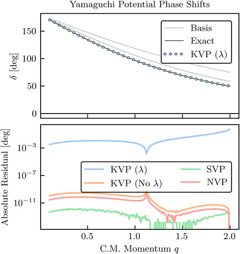
FIGURE 9. Phase shifts (top panel) and absolute residuals (bottom panel) in arbitrary units for the Yamaguchi potential Eq. 87 for each scattering emulator discussed above. The solid black lines represent the high-fidelity solution and the dots represent the emulator results. The emulators are so accurate that they are indistinguishable unless looking at residuals. The training set is given by the two gray lines.

Figure 10 shows the high-fidelity (solid black line), emulated (dots), and basis (solid gray line) wave functions for three values of q with their absolute residuals using the constrained KVP constructed with n_b = 5 training points. The emulator reproduces the high-fidelity solution at all three values of q, with q = 2.0 having the smallest residual. The sensitivity of the emulator accuracy as n_b is varied can be readily studied using the Python code provided on the companion website [20]. An example of how the accuracy is affected when varying n_b is also given in Ref. [88].

FIGURE 10

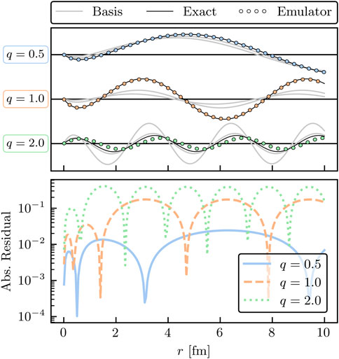
FIGURE 10. Wave functions (top panel) and absolute residuals (bottom panel) for the Yamaguchi potential Eq. 87 in arbitrary units using the constrained KVP. The top panel legend description is similar to Figure 9, but for three different values of q. The bottom panel shows the relative residuals of the three values previously mentioned.

While all emulators described in this Section are applicable to scattering problems in general, their efficacy will depend in practice on various factors, such as their computational complexity and the potential to be emulated. The constrained KVP has the advantage that terms constant in θ, such as the (long-range) Coulomb potential, cancel in the computation of Eq. 33 but it loses one degree of freedom due to the normalization constraint of the coefficients. On the other hand, both the NVP and SVP involve the computation of Green’s functions, which makes them computationally more complex than the KVP—especially the SVP since it also depends quadratically on the potential.

5 Summary and outlook

We have presented a pedagogical introduction to projection-based, reduced-order emulators and general MOR concepts suitable for a wide range of applications in low-energy nuclear physics. Emulators are fast surrogate models capable of reliably approximating high-fidelity models due to their reduced content of superfluous information. By making practical otherwise impractical calculations, they can open the door to the various techniques and applications central to the overall theme of this Frontiers Research Topic [14], such as Bayesian parameter estimation for UQ, experimental design, and many more.

In particular, we have discussed variational and Galerkin methods combined with snapshot-based trial (or test) functions as the foundation for constructing fast and accurate emulators. These emulators enable repeated bound state and scattering calculations, e.g., for sampling a model’s parameter space when high-fidelity calculations are computationally expensive or prohibitively slow. A crucial element in this emulator workflow, as summarized in Figure 2, is an efficient offline-online decomposition in which the heavy computational lifting is performed only once before the emulator is invoked. Chiral Hamiltonians allow for such efficient decompositions due to their affine parameter dependence on the low-energy couplings. Furthermore, we discussed the high efficacy of projection-based emulators in extrapolating results far from the support of the snapshot data, as opposed to the GPs.

While MOR has already reached maturity in other fields, it is still in its infancy in nuclear physics—although rapidly growing—and there remains much to explore and exploit [18, 35, 36, 43]. In the following, we highlight some of the many interesting research avenues for emulator applications in nuclear physics. All of these avenues can benefit from the rich MOR literature and software tools available (e.g., see Refs. [1–3]):

• Emulator uncertainties need to be robustly quantified and treated on equal footing with other uncertainties in nuclear physics calculations, such as EFT truncation errors. This will be facilitated by the extensive literature on the uncertainties in the RBM [76, 77, 90, 111].

• The performance of competing emulators (e.g., the Newton vs. Kohn variational principle) is typically highly implementation dependent. Best practices for efficient implementation of nuclear physics emulators should be developed. This may include exploiting MOR software libraries from other fields, such as pyMOR [112], when possible.

• Galerkin emulators are equivalent to variational emulators for bound-state and scattering calculations if the test and trial basis are properly chosen. But Galerkin (and especially Petrov-Galerkin) emulators are more general and exploring their applications in non-linear problems may be fruitful in nuclear physics. Emulator applied to non-linear problems will have challenges in terms of both speed and accuracy: 1) the basis size will, in general, need to be large(r) resulting in lower speed-up factors and longer offline stages; 2) using hyperreduction methods will lead to additional approximations that worsen the accuracy of the emulator and whose uncertainties need to be quantified.

• Many technical aspects should be further explored, such as greedy (or active-learning) [24] and SVD-based algorithms for choosing the training points more effectively, hyperreduction methods for non-affine problems, and improved convergence analyses.

• Scattering emulators could play pivotal roles in connecting reaction models and experiments at new-generation rare-isotope facilities (e.g., the Facility for Rare Isotope Beams). In this regard, further studies on incorporating long-range Coulomb interactions and optical potentials beyond two-body systems will be valuable. Furthermore, emulators for time-dependent density functional theories could see extensive applications in interpreting fission measurements. At facilities such as Jefferson Lab and the future Electron-Ion Collider, explorations of nuclear dynamics at much higher energy scales should also benefit from emulators.

• The emulator framework can be used to extrapolate observables far away from the support of the training data, such as the discrete energy levels of a many-body system calculated in one phase to those of another, as demonstrated in Ref. [22]. Using emulators as a resummation tool to increase the convergence radius of series expansions [26] falls into this category as well, and so does using them to extrapolate finite-box simulations of quantum systems across wide ranges of box sizes [40]. Moreover, for general quantum continuum states, emulation in the complex energy plane can enable computing scattering observables with bound-state methods [113]. Extrapolation capabilities of emulators should be investigated further.

• While projection-based emulators have had successes (e.g., see Refs. [7, 9, 25]), it is also important to understand their limitations and investigate potential improvements. The synergy between projection-based and machine learning methods [114] is a new direction being undertaken in the field of MOR for this purpose (e.g., see Ref. [63]). Nuclear physics problems, with and without time dependence, will provide ample opportunities for such explorations.

• Emulators run fast, often with a small memory footprint, and can be easily shared. These properties make emulators effective interfaces for large expensive calculations, through which users can access sophisticated physical models at a minimum cost of computational resources and without specialized expertise, creating a more efficient workflow for nuclear science. As such, emulators can become a collaboration tool [33, 34] that can catalyze new direct and indirect connections between different research areas and enable novel studies.

To help foster the exploration of these (and other) research directions in nuclear physics, we have created a companion website [20] containing interactive supplemental material and source code so that the interested reader can experiment with and extend the examples discussed here.

We look forward to seeing more of the MOR methodology implemented as these research directions are being pursued. But especially we look forward to the exciting applications of emulators in nuclear physics that are currently beyond our grasp.

Author contributions

All authors listed have made a substantial, direct, and intellectual contribution to the work and approved it for publication.

Funding

This material is based upon work supported by the U.S. Department of Energy, Office of Science, Office of Nuclear Physics, under the FRIB Theory Alliance award DE-SC0013617. This work was supported in part by the National Science Foundation under award numbers PHY-1913069 and PHY-2209442 and the NSF CSSI program under award number OAC-2004601 (BAND Collaboration [115]), and the NUCLEI SciDAC Collaboration under U.S. Department of Energy MSU subcontract RC107839-OSU.

Acknowledgments

We thank the Editors Maria Piarulli, Evgeny Epelbaum, and Christian Forssén for the kind invitation to contribute to this Frontiers Research Topic [14]. We are also grateful to our BUQEYE [19] and BAND [115] collaboration colleagues for sharing their invaluable insights with us, and especially to Pablo Giuliani and Daniel Phillips for fruitful discussions. C.D. thanks Petar Mlinarić for sharing his deep insights into the software library pyMOR [112] for building MOR applications with the Python.

Conflict of interest

The authors declare that the research was conducted in the absence of any commercial or financial relationships that could be construed as a potential conflict of interest.

Publisher’s note

All claims expressed in this article are solely those of the authors and do not necessarily represent those of their affiliated organizations, or those of the publisher, the editors and the reviewers. Any product that may be evaluated in this article, or claim that may be made by its manufacturer, is not guaranteed or endorsed by the publisher.

Footnotes

¹A reliable emulator may not necessarily be required to be highly accurate, e.g., if the other uncertainties of the theoretical calculation dominate the overall uncertainty budget

²For a critical commentary on the history of the method’s name, see, e.g., Refs. [45, 46].

³Many helpful theorems relevant to the Rayleigh–Ritz method can be found in Section 3 in Ref. [47].

⁴In a representation of H, the ψ_i corresponding to |ψ_i⟩ are the n_b columns of the matrix X in that representation

⁵For non-Hermitian Hamiltonians, one generally does not obtain the variational bounds (Eq. 7) as can be observed in, e.g., the subspace-projected coupled-cluster method developed in Ref. [7].

⁶For simplicity we consider ξ to be a real variable; for complex variables, independent variations $\delta {\vec{\beta }}^{*}$ should be included in the discussion

⁷We focus here on examples with real-valued potentials and without long-range Coulomb interactions. Cases with complex-valued potentials and/or the Coulomb interaction may be analyzed in similar ways; relevant discussions specific to Kohn emulators can be found in Refs. [30, 32].

⁸Note that left-multiplying by V(θ) and enforcing orthogonality against |ζ_i⟩ = |ψ_i⟩ is different than simply defining |ζ⟩ = V|ψ⟩ and enforcing orthogonality against |ζ_i⟩ = V_i|ψ_i⟩ because V(θ) depends on θ. Thus, this is indeed a purely Galerkin approach, rather than a Petrov-Galerkin approach

⁹We follow the conventions for scattering matrices in Refs. [99, 100]. Thus, the K matrix in this section is dimensionless and defined without the negative sign in Eq. 28.

¹⁰These anomalies are not restricted to the KVP but also appear in other VPs such as the NVP and SVP [102].

¹¹The other high-fidelity solvers in this context solve problems in momentum or coordinate space based on the Faddeev formalism [105–107].

References

1. Benner P, Ohlberger M, Patera A, Rozza G, Urban K. Reduction of parametrized systems. Berlin, Germany: Springer (2017).

Google Scholar

2. Benner P, Cohen A, Ohlberger M, Willcox K. Reduction and approximation. Philadelphia, PA: Society for Industrial and Applied Mathematics: Computational Science & Engineering (2017).

Google Scholar

3. Benner P, Gugercin S, Willcox K. A survey of projection-based model reduction methods for parametric dynamical systems. SIAM Rev (2015) 57:483–531. doi:10.1137/130932715

CrossRef Full Text | Google Scholar

4. Zhang X, Nollett KM, Phillips DR. Halo effective field theory constrains the solar ⁷Be + p → ⁸B + γ rate. Phys Lett B (2015) 751:535–40. arXiv:1507.07239. doi:10.1016/j.physletb.2015.11.005

CrossRef Full Text | Google Scholar

5. Neufcourt L, Cao Y, Nazarewicz W, Olsen E, Viens F. Neutron drip line in the Ca region from bayesian model averaging. Phys Rev Lett (2019) 122:062502. arXiv:1901.07632 [nucl-th]. doi:10.1103/physrevlett.122.062502

PubMed Abstract | CrossRef Full Text | Google Scholar

6. King GB, Lovell AE, Neufcourt L, Nunes FM. Direct comparison between bayesian and frequentist uncertainty quantification for nuclear reactions. Phys Rev Lett (2019) 122:232502. arXiv:1905.05072 [nucl-th]. doi:10.1103/physrevlett.122.232502

PubMed Abstract | CrossRef Full Text | Google Scholar

7. Ekström A, Hagen G. Global sensitivity analysis of bulk properties of an atomic nucleus. Phys Rev Lett (2019) 123:252501. arXiv:1910.02922 [nucl-th]. doi:10.1103/physrevlett.123.252501

PubMed Abstract | CrossRef Full Text | Google Scholar

8. Catacora-Rios M, King GB, Lovell AE, Nunes FM. Statistical tools for a better optical model. Phys Rev C (2021) 104:064611. arXiv:2012.06653 [nucl-th]. doi:10.1103/physrevc.104.064611

CrossRef Full Text | Google Scholar

9. Wesolowski S, Svensson I, Ekström A, Forssén C, Furnstahl RJ, Melendez JA, et al. Rigorous constraints on three-nucleon forces in chiral effective field theory from fast and accurate calculations of few-body observables. Phys Rev C (2021) 104:064001. arXiv:2104.04441 [nucl-th]. doi:10.1103/physrevc.104.064001

CrossRef Full Text | Google Scholar

10. Svensson I, Ekström A, Forssén C. Bayesian parameter estimation in chiral effective field theory using the Hamiltonian Monte Carlo method. Phys Rev C (2022) 105:014004. arXiv:2110.04011 [nucl-th]. doi:10.1103/physrevc.105.014004

CrossRef Full Text | Google Scholar

11. Odell D, Brune CR, Phillips DR, deBoer RJ, Paneru SN. Performing bayesian analyses with AZURE2 using BRICK: An application to the 7Be system. Phys Rev C (2022) 105:014625. arXiv:2105.06541 [nucl-th]. doi:10.3389/fphy.2022.888476

CrossRef Full Text | Google Scholar

12. Djärv T, Ekström A, Forssén C, Johansson HT. Candidate entanglement invariants for two Dirac spinors. Phys Rev C (2022) 105:032402. arXiv:2108.13313 [nucl-th]. doi:10.1103/physreva.105.032402

CrossRef Full Text | Google Scholar

13. Alnamlah IK, Pérez EAC, Phillips DR. Analyzing rotational bands in odd-mass nuclei using effective field theory and Bayesian methods. Front Phys (2022) 10:901954. arXiv:2203.01972 [nucl-th]. doi:10.3389/fphy.2022.901954

CrossRef Full Text | Google Scholar

14.Frontiers in Physics. Research topic: Uncertainty quantification in nuclear physics (2022) (Online; accessed November 2, 2022)

Google Scholar

15. Phillips DR, Furnstahl RJ, Heinz U, Maiti T, Nazarewicz W, Nunes FM, et al. Get on the BAND wagon: A bayesian framework for quantifying model uncertainties in nuclear dynamics. J Phys G (2021) 48:072001. arXiv:2012.07704 [nucl-th]. doi:10.1088/1361-6471/abf1df

CrossRef Full Text | Google Scholar

16. Melendez JA, Furnstahl RJ, Grießhammer HW, McGovern JA, Phillips DR, Pratola MT. Designing optimal experiments: An application to proton compton scattering. Eur Phys J A (2021) 57:81. arXiv:2004.11307 [nucl-th]. doi:10.1140/epja/s10050-021-00382-2

CrossRef Full Text | Google Scholar

17. Farr JN, Meisel Z, Steiner AW. Decision theory for the mass measurements at the facility for rare isotope beams. arXiv:2111.11536 [nucl-th]. doi:10.48550/arXiv.2111.11536

CrossRef Full Text | Google Scholar

18. Melendez JA, Drischler C, Furnstahl RJ, Garcia AJ, Zhang X. Model reduction methods for nuclear emulators. J Phys G (2022) 49:102001. arXiv:2203.05528 [nucl-th]. doi:10.1088/1361-6471/ac83dd

CrossRef Full Text | Google Scholar

19.BUQEYE collaboration. Buqeye (2021). Available at: https://buqeye.github.io/ (Accessed December 15, 2022).

Google Scholar

20.BUQEYE collaboration. Frontiers emulator review (2022). Available at: https://github.com/buqeye/frontiers-emulator-review (Accessed December 15, 2022).

Google Scholar

21. Higdon D, McDonnell JD, Schunck N, Sarich J, Wild SM. A Bayesian approach for parameter estimation and prediction using a computationally intensive model. J Phys G (2015) 42:034009. arXiv:1407.3017. doi:10.1088/0954-3899/42/3/034009

CrossRef Full Text | Google Scholar

22. Frame D, He R, Ipsen I, Lee D, Lee D, Rrapaj E. Eigenvector continuation with subspace learning. Phys Rev Lett (2018) 121:032501. arXiv:1711.07090. doi:10.1103/physrevlett.121.032501

PubMed Abstract | CrossRef Full Text | Google Scholar

23. Sarkar A, Lee D. Convergence of eigenvector continuation. Phys Rev Lett (2021) 126:032501. arXiv:2004.07651 [nucl-th]. doi:10.1103/physrevlett.126.032501

PubMed Abstract | CrossRef Full Text | Google Scholar

24. Sarkar A, Lee D. Self-learning emulators and eigenvector continuation. Phys Rev Res (2022) 4:023214. arXiv:2107.13449 [nucl-th]. doi:10.1103/physrevresearch.4.023214

CrossRef Full Text | Google Scholar

25. König S, Ekström A, Hebeler K, Lee D, Schwenk A. Eigenvector continuation as an efficient and accurate emulator for uncertainty quantification. Phys Lett B (2020) 810:135814. arXiv:1909.08446 [nucl-th]. doi:10.1016/j.physletb.2020.135814

CrossRef Full Text | Google Scholar

26. Demol P, Duguet T, Ekström A, Frosini M, Hebeler K, König S, et al. Improved many-body expansions from eigenvector continuation. Phys Rev C (2020) 101:041302. arXiv:1911.12578. doi:10.1103/physrevc.101.041302

CrossRef Full Text | Google Scholar

27. Bai D, Ren Z. Generalizing the calculable R-matrix theory and eigenvector continuation to the incoming-wave boundary condition. Phys Rev C (2021) 103:014612. arXiv:2101.06336 [nucl-th]. doi:10.1103/physrevc.103.014612

CrossRef Full Text | Google Scholar

28. Demol P, Frosini M, Tichai A, Somà V, Duguet T. Bogoliubov many-body perturbation theory under constraint. Ann Phys (2021) 424:168358. arXiv:2002.02724 [nucl-th]. doi:10.1016/j.aop.2020.168358

CrossRef Full Text | Google Scholar

29. Yoshida S, Shimizu N. Constructing approximate shell-model wavefunctions by eigenvector continuation. arXiv:2105.08256 [nucl-th]. doi:10.48550/arXiv.2105.08256

CrossRef Full Text | Google Scholar

30. Furnstahl RJ, Garcia AJ, Millican PJ, Zhang X. Efficient emulators for scattering using eigenvector continuation. Phys Lett B (2020) 809:135719. arXiv:2007.03635 [nucl-th]. doi:10.1016/j.physletb.2020.135719

CrossRef Full Text | Google Scholar

31. Melendez J, Drischler C, Garcia A, Furnstahl R, Zhang X. Fast and accurate emulation of two-body scattering observables without wave functions. Phys Lett B (2021) 821:136608. doi:10.1016/j.physletb.2021.136608

CrossRef Full Text | Google Scholar

32. Drischler C, Quinonez M, Giuliani PG, Lovell AE, Nunes FM. Toward emulating nuclear reactions using eigenvector continuation. Phys Lett B (2021) 823:136777. arXiv:2108.08269 [nucl-th]. doi:10.1016/j.physletb.2021.136777

CrossRef Full Text | Google Scholar

33. Zhang X, Furnstahl RJ. Fast emulation of quantum three-body scattering. Phys Rev C (2021) 105:064004. arXiv:2110.04269 [nucl-th]. doi:10.1103/physrevc.105.064004

CrossRef Full Text | Google Scholar

34. Tews I, Davoudi Z, Ekström A, Holt JD, Becker K, Briceño R, et al. Nuclear forces for precision nuclear physics – A collection of perspectives. Few-Body Syst (2022) 63:67. arXiv:2202.01105. doi:10.1007/s00601-022-01749-x

CrossRef Full Text | Google Scholar

35. Anderson AL, O’Donnell GL, Piekarewicz J. Applications of reduced-basis methods to the nuclear single-particle spectrum. Phys Rev C (2022) 106:L031302. arXiv:2206.14889 [nucl-th]. doi:10.1103/physrevc.106.l031302

CrossRef Full Text | Google Scholar

36. Giuliani P, Godbey K, Bonilla E, Viens F, Piekarewicz J. Bayes goes fast: Uncertainty quantification for a covariant energy density functional emulated by the reduced basis method. Front. Phys. (2022) 13039. arXiv:2209[nucl-th]. doi:10.48550/arXiv.2209.13039

CrossRef Full Text | Google Scholar

37. Sürer O, Nunes FM, Plumlee M, Wild SM. Uncertainty quantification in breakup reactions. Phys Rev C (2022) 106:024607. arXiv:2205.07119 [nucl-th]. doi:10.1103/physrevc.106.024607

CrossRef Full Text | Google Scholar

38. Bai D, Ren Z. Entanglement generation in few-nucleon scattering. Phys Rev C (2022) 106:064005. doi:10.1103/physrevc.106.064005

CrossRef Full Text | Google Scholar

39. Kravvaris K, Quinlan KR, Quaglioni S, Wendt KA, Navratil P. Quantifying uncertainties in neutron-α scattering with chiral nucleon-nucleon and three-nucleon forces. Phys Rev C (2020) 102:024616. arXiv:2004.08474 [nucl-th]. doi:10.1103/physrevc.102.024616

CrossRef Full Text | Google Scholar

40. Yapa N, König S. Volume extrapolation via eigenvector continuation. Phys Rev C (2022) 106:014309. arXiv:2201.08313 [nucl-th]. doi:10.1103/physrevc.106.014309

CrossRef Full Text | Google Scholar

41. Francis A, Agrawal AA, Howard JH, Kökcü E, Kemper AF. Subspace diagonalization on quantum computers using eigenvector continuation. 10571. arXiv:2209[quant-ph]. doi:10.48550/arXiv.2209.10571

CrossRef Full Text | Google Scholar

42. Zare A, Wirth R, Haselby CA, Hergert H, Iwen M. Modewise johnson-lindenstrauss embeddings for nuclear many-body theory. 01305. arXiv:2211. doi:10.48550/arXiv.2211.01305

CrossRef Full Text | Google Scholar

43. Bonilla E, Giuliani P, Godbey K, Lee D. Training and projecting: A reduced basis method emulator for many-body physics. Phys Rev C (2022) 106:054322. arXiv:2203.05284 [nucl-th]. doi:10.1103/physrevc.106.054322

CrossRef Full Text | Google Scholar

44. Benner P, Schilders W, Grivet-Talocia S, Quarteroni A, Rozza G, Miguel Silveira L. System- and data-driven methods and algorithms. Berlin, Germany: De Gruyter (2021).

Google Scholar

45. Leissa A. The historical bases of the Rayleigh and Ritz methods. J Sound Vibration (2005) 287:961–78. doi:10.1016/j.jsv.2004.12.021

CrossRef Full Text | Google Scholar

46. Ilanko S. Comments on the historical bases of the Rayleigh and Ritz methods. J Sound Vibration (2009) 319:731–3. doi:10.1016/j.jsv.2008.06.001

CrossRef Full Text | Google Scholar

47. Suzuki Y, Varga K. Stochastic variational approach to quantum-mechanical few-body problems. Berlin, Germany: Springer Berlin Heidelberg (1998).

Google Scholar

48. Benner P, Schilders W, Grivet-Talocia S, Quarteroni A, Rozza G, Miguel Silveira L. Order reduction: Volume 2: Snapshot-based methods and algorithms. Berlin, Germany: De Gruyter (2020). p. 1–348.

Google Scholar

49. Buchan AG, Pain CC, Fang F, Navon IM. A POD reduced-order model for eigenvalue problems with application to reactor physics. Int J Numer Methods Eng (2013) 95:1011–32. doi:10.1002/nme.4533

CrossRef Full Text | Google Scholar

50. Quarteroni A, Manzoni A, Negri F. Reduced basis methods for partial differential equations. In: An Introduction, La Matematica per il 3+2. Berlin, Germany: Springer International Publishing (2016). p. 92.

CrossRef Full Text | Google Scholar

51. Franzke MC, Tichai A, Hebeler K, Schwenk A. Excited states from eigenvector continuation: The anharmonic oscillator. Phys Lett B (2022) 830:137101. arXiv:2108.02824. doi:10.1016/j.physletb.2022.137101

CrossRef Full Text | Google Scholar

52. Melendez J. Effective field theory truncation errors and why they matter. Ph.D. thesis. Columbus, Ohio: Ohio State U. (2020).

53. Hicks C, Lee D. Trimmed sampling algorithm for the noisy generalized eigenvalue problem. 02083. arXiv:2209. doi:10.48550/arXiv.2209.02083

CrossRef Full Text | Google Scholar

54. Neumaier A. Solving ill-conditioned and singular linear systems: A tutorial on regularization. SIAM Rev (1998) 40:636–66. doi:10.1137/s0036144597321909

CrossRef Full Text | Google Scholar

55. Engl H, Hanke M, Neubauer A. Regularization of inverse problems. In: Mathematics and its applications. Netherlands: Springer (1996).

Google Scholar

56. Hergert H. A guided tour of ab initio nuclear many-body theory. Front Phys (2020) 8:37905061. arXiv:2008. doi:10.3389/fphy.2020.00379

CrossRef Full Text | Google Scholar

57. Ghattas O, Willcox K. Learning physics-based models from data: Perspectives from inverse problems and model reduction. Acta Numerica (2021) 30:445–554. doi:10.1017/s0962492921000064

CrossRef Full Text | Google Scholar

58. Rasmussen CE, Williams CKI. Gaussian processes for machine learning, adaptive computation and machine learning series. Cambridge, MA: University Press Group Limited (2006).

Google Scholar

59. Mezić I. Analysis of fluid flows via spectral properties of the koopman operator. Annu Rev Fluid Mech (2013) 45:357–78. doi:10.1146/annurev-fluid-011212-140652

CrossRef Full Text | Google Scholar

60. Kutz JN, Brunton SL, Brunton BW, Proctor JL. Dynamic mode decomposition. In: Other titles in applied mathematics. Pennsylvania, United States: SIAM-Society for Industrial and Applied Mathematics (2016).

Google Scholar

61. Raissi M, Perdikaris P, Karniadakis GE. Physics-informed neural networks: A deep learning framework for solving forward and inverse problems involving nonlinear partial differential equations. J Comput Phys (2019) 378:686–707. doi:10.1016/j.jcp.2018.10.045

CrossRef Full Text | Google Scholar

62. Chen W, Wang Q, Hesthaven JS, Zhang C. Physics-informed machine learning for reduced-order modeling of nonlinear problems. J Comput Phys (2021) 446:110666. doi:10.1016/j.jcp.2021.110666

CrossRef Full Text | Google Scholar

63. Fresca S, Manzoni A. POD-DL-ROM: Enhancing deep learning-based reduced order models for nonlinear parametrized PDEs by proper orthogonal decomposition. Comp Methods Appl Mech Eng (2022) 388:114181. doi:10.1016/j.cma.2021.114181

CrossRef Full Text | Google Scholar

64. Hesthaven J, Rozza G, Stamm B. Certified reduced basis methods for parametrized partial differential equations. In: SpringerBriefs in mathematics. Berlin, Germany: Springer International Publishing (2015).

Google Scholar

65. Barrault M, Maday Y, Nguyen NC, Patera AT. An ‘empirical interpolation’ method: Application to efficient reduced-basis discretization of partial differential equations. Comptes Rendus Mathematique (2004) 339:667–72. doi:10.1016/j.crma.2004.08.006

CrossRef Full Text | Google Scholar

66. Grepl MA, Maday Y, Nguyen NC, Patera AT. Efficient reduced-basis treatment of nonaffine and nonlinear partial differential equations. ESAIM: M2AN (2007) 41:575–605. doi:10.1051/m2an:2007031

CrossRef Full Text | Google Scholar

67. Horacio LC, Solis-Daun J. Synthesis of positive controls for the global CLF stabilization of systems. In: Proceedings of the 48h IEEE Conference on Decision and Control (CDC) held jointly with 2009 28th Chinese Control Conference; 15-18 December 2009; Shanghai, China (2009). p. 4316–21.

Google Scholar

68. Chaturantabut S, Sorensen DC. Nonlinear model reduction via discrete empirical interpolation. SIAM J Scientific Comput (2010) 32:2737–64. doi:10.1137/090766498

CrossRef Full Text | Google Scholar

69. Bui-Thanh T, Damodaran M, Willcox K. Proper orthogonal decomposition extensions for parametric applications in compressible aerodynamics. In: 21st AIAA Applied Aerodynamics Conference; 23 June 2003 - 26 June 2003; Orlando, Florida (2003).

CrossRef Full Text | Google Scholar

70. Carlberg K, Bou-Mosleh C, Farhat C. Efficient non-linear model reduction via a least-squares Petrov-Galerkin projection and compressive tensor approximations. Int J Numer Methods Eng (2011) 86:155–81. doi:10.1002/nme.3050

CrossRef Full Text | Google Scholar

71. Amsallem D, Cortial J, Farhat C. Towards real-time computational-fluid-dynamics-based aeroelastic computations using a database of reduced-order information. AIAA J (2010) 48:2029–37. doi:10.2514/1.j050233

CrossRef Full Text | Google Scholar

72. An SS, Kim T, James DL. Session details: Character animation II. ACM Trans Graph (2008) 27:3262975. doi:10.1145/3262975

CrossRef Full Text | Google Scholar

73. Farhat C, Avery P, Chapman T, Cortial J. Dimensional reduction of nonlinear finite element dynamic models with finite rotations and energy-based mesh sampling and weighting for computational efficiency. Int J Numer Methods Eng (2014) 98:625–62. doi:10.1002/nme.4668

CrossRef Full Text | Google Scholar

74. Guo M, Hesthaven JS. Reduced order modeling for nonlinear structural analysis using Gaussian process regression. Comp Methods Appl Mech Eng (2018) 341:807–26. doi:10.1016/j.cma.2018.07.017

CrossRef Full Text | Google Scholar

75. Gubisch M, Volkwein S. Chapter 1: Proper orthogonal decomposition for linear-quadratic optimal control. In: Reduction and approximation (2017). p. 3–63.

CrossRef Full Text | Google Scholar

76. Rozza G, Huynh DBP, Patera AT. Reduced basis approximation and a posteriori error estimation for affinely parametrized elliptic coercive partial differential equations. Arch Comput Methods Eng (2008) 15:229–75. doi:10.1007/s11831-008-9019-9

CrossRef Full Text | Google Scholar

77. Chen P, Quarteroni A, Rozza G. Reduced basis methods for uncertainty quantification. SIAM/ASA J Uncertainty Quantification (2017) 5:813–69. doi:10.1137/151004550

CrossRef Full Text | Google Scholar

78. Horger T, Wohlmuth B, Thomas D. Simultaneous reduced basis approximation of parameterized elliptic eigenvalue problems. ESAIM: M2AN (2017) 51:443–65. doi:10.1051/m2an/2016025

CrossRef Full Text | Google Scholar

79. MacKay DJC. Neural networks and machine learning. In: CM Bishop, editor. NATO ASI series. Berlin: Springer (1998). p. 133–66.

Google Scholar

80. MacKay DJC. Information theory, inference, and learning algorithms. Cambridge, UK: Cambridge University Press (2003).

Google Scholar

81. Gander MJ, Wanner G. From euler, Ritz, and Galerkin to modern computing. SIAM Rev (2012) 54:627–66. doi:10.1137/100804036

CrossRef Full Text | Google Scholar

82. Zienkiewicz O, Taylor R, Zhu J. The finite element method: Its basis and fundamentals. 7th ed. Oxford: Butterworth-Heinemann (Butterworth-Heinemann (2013).

Google Scholar

83. Zienkiewicz O, Taylor R, Fox D. The finite element method for solid and structural mechanics. 7th ed. Oxford: Butterworth-Heinemann (2014).

Google Scholar

84. Zienkiewicz O, Taylor R, Nithiarasu P. The finite element method for fluid dynamics. 7th ed. Oxford: Butterworth-Heinemann (2014).

Google Scholar

85. Mikhlin SG. Variational methods in mathematical physics. Oxford: Cambridge University Press (1967). [Translated by T. Boddington for Pergamon Press, Oxford, 1964].

Google Scholar

86. Evans JD. Straightforward statistics for the behavioral sciences. Pacific Grove, CA: Brooks/Cole Publishing (1996).

Google Scholar

87. Brenner SC, Scott LR. The mathematical theory of finite element methods. In: Texts in applied mathematics. Berlin, Germany: Springer (2008).

Google Scholar

88. Garcia AJ, Drischler C, Furnstahl RJ, Melendez JA, Zhang X. Wave function-based emulation for nucleon-nucleon scattering in momentum space. arXiv:2301.05093.

Google Scholar

89. Benner P, Schilders W, Grivet-Talocia S, Quarteroni A, Rozza G, Miguel Silveira L. Order reduction: Volume 3: Applications. Berlin, Germany: De Gruyter (2020).

Google Scholar

90. Huynh D, Rozza G, Sen S, Patera A. A successive constraint linear optimization method for lower bounds of parametric coercivity and inf–sup stability constants. Comptes Rendus Mathematique (2007) 345:473–8. doi:10.1016/j.crma.2007.09.019

CrossRef Full Text | Google Scholar

91. Kohn W. Variational methods in nuclear collision problems. Phys Rev (1948) 74:1763–72. doi:10.1103/physrev.74.1763

CrossRef Full Text | Google Scholar

92. Kohn W. Variational scattering theory in momentum space I. Central field problems. Phys Rev (1951) 84:495–501. doi:10.1103/physrev.84.495

CrossRef Full Text | Google Scholar

93. Drischler C, Holt JW, Wellenhofer C. Chiral effective field theory and the high-density nuclear equation of state. Annu Rev Nucl Part Sci (2021) 71:403–32. arXiv:2101.01709. doi:10.1146/annurev-nucl-102419-041903

CrossRef Full Text | Google Scholar

94. Takatsuka K, Lucchese RR, McKoy V. Relationship between the schwinger and kohn-type variational principles in scattering theory. Phys Rev A (1981) 24:1812–6. doi:10.1103/physreva.24.1812

CrossRef Full Text | Google Scholar

95. Takatsuka K, McKoy V. Variational scattering theory using a functional of fractional form. I. General theory. Phys Rev A (1981) 23:2352–8. doi:10.1103/physreva.23.2352

CrossRef Full Text | Google Scholar

96. Newton RG. Scattering theory of waves and particles. Illinois, United States: Dover (2002).

Google Scholar

97. Thompson IJ, Nunes FM. Nuclear reactions for astrophysics: Principles, calculation and applications of low-energy reactions. Cambridge, United Kingdom: Cambridge University Press (2009).

Google Scholar

98. Lucchese RR. Anomalous singularities in the complex kohn variational principle of quantum scattering theory. Phys Rev A (1989) 40:6879–85. doi:10.1103/physreva.40.6879

CrossRef Full Text | Google Scholar

99. Taylor JR. Scattering theory: The quantum theory of nonrelativistic collisions. Illinois, United States: Dover (2006).

Google Scholar

100. Morrison MA, Feldt AN. Through scattering theory with gun and camera: Coping with conventions in collision theory. Am J Phys (2007) 75:67–80. doi:10.1119/1.2358156

CrossRef Full Text | Google Scholar

101. Nesbet R. Variational methods in electron-atom scattering theory, Physics of atoms and molecules. Plenum Press (1980).

Google Scholar

102. Adhikari SK. Anomalies of variational phase shifts. Chem Phys Lett (1991) 181:435–40. doi:10.1016/0009-2614(91)90376-k

CrossRef Full Text | Google Scholar

103. Marcucci LE, Dohet-Eraly J, Girlanda L, Gnech A, Kievsky A, Viviani M. The hyperspherical harmonics method: A tool for testing and improving nuclear interaction models. Front Phys (2020) 8:69. arXiv:1912.09751 [nucl-th]. doi:10.3389/fphy.2020.00069

CrossRef Full Text | Google Scholar

104. Kievsky A, Rosati S, Viviani M, Marcucci LE, Girlanda L. A high-precision variational approach to three- and four-nucleon bound and zero-energy scattering states. J Phys G (2008) 35:063101. arXiv:0805.4688. doi:10.1088/0954-3899/35/6/063101

CrossRef Full Text | Google Scholar

105. Gloeckle W, Witala H, Huber D, Kamada H, Golak J. A New look into the partial wave decomposition of three nucleon forces. Phys Rept (1996) 274:107. doi:10.1007/s006010050057

CrossRef Full Text | Google Scholar

106. Deltuva A, Fonseca AC, Lazauskas R. Faddeev equation approach for three-cluster nuclear reactions. In: Lecture notes in physics. Berlin, Germany: Springer (2014). p. 1. arXiv:1201.4979 [nucl-th].

CrossRef Full Text | Google Scholar

107. Lazauskas R, Carbonell J. The faddeev–yakubovsky symphony. Few Body Syst (2019) 60:62. arXiv:1908.04861 [quant-ph]. doi:10.1007/s00601-019-1529-5

CrossRef Full Text | Google Scholar

108. Tabakin F. Inverse scattering problem for separable potentials. Phys Rev (1969) 177:1443–51. doi:10.1103/physrev.177.1443

CrossRef Full Text | Google Scholar

109. Kwong NH, Köhler HS. SeparableNNpotentials from inverse scattering for nuclear matter studies. Phys Rev C (1997) 55:1650–64. doi:10.1103/physrevc.55.1650

CrossRef Full Text | Google Scholar

110. Göbel M, Hammer HW, Ji C, Phillips DR. Momentum-space probability density of {}^6He in halo effective field theory. Few Body Syst (2019) 60:61. arXiv:1904.07182 [nucl-th]. doi:10.1007/s00601-019-1528-6

CrossRef Full Text | Google Scholar

111. Haasdonk B. Chapter 2: Reduced basis methods for parametrized pdes—A tutorial introduction for stationary and instationary problems. In: Reduction and approximation. Philadelphia, PA: Computational Science & Engineering (2017). p. 65–136.

CrossRef Full Text | Google Scholar

112. Milk R, Rave S, Schindler F. pyMOR -- generic algorithms and interfaces for model order reduction. SIAM J Scientific Comput (2016) 38:S194–216. doi:10.1137/15m1026614

CrossRef Full Text | Google Scholar

113.Zhang X, Low Energy Community Meeting. Recent developments in the emulations of quantum continuum states. USA: Argonne National Laboratory (2022).

Google Scholar

114. Boehnlein A, Diefenthaler M, Sato N, Schram M, Ziegler V, Fanelli C, et al. Colloquium: Machine learning in nuclear physics. Rev Mod Phys (2022) 94:031003. arXiv:2112.02309 [nucl-th]. doi:10.1103/revmodphys.94.031003

CrossRef Full Text | Google Scholar

115.BAND. Bayesian analysis of nuclear dynamics (BAND) framework project (2020). Available at: https://bandframework.github.io/ (Accessed December 15, 2022).

Google Scholar