Application of reinforcement learning in the LHC tune feedback

1 Introduction

The LHC is the largest synchrotron built to date and its sheer scale meant that it was the first particle accelerator of its type to require automatic beam-based feedback systems to control key beam parameters [1]. The Beam-Based Feedback System (BBFS) implemented these feedback systems and was developed prior to the LHC start-up in 2008. Throughout the years, operator experience has dictated which functionality to keep, add and remove from the BBFS [2].

The BBFS comprised several subsystems, each responsible for controlling a specific beam parameter or machine parameter. One of the most critical parameters to control is the tune (Q). Q is defined as the number of transverse oscillations a particle performs in one revolution around the LHC. Ideally the value of the tune is an irrational number so that the location of the transverse oscillations do not occur in the same longitudinal locations in the LHC. The Tune Feedback (QFB) system was the BBFS subsystem responsible for controlling the tune.

The QFB requires a constantly updated estimate of the value of the tunes in the horizontal and vertical planes of both beams in the LHC. The estimation of the tune was performed by the Base-Band Tune (BBQ) system [3]. Each plane in every beam was handled independently through a set of tuning quadrupoles of type MQT, to adjust the magnetic beam envelope. The QFB operated on the assumption that the effect of a changing quadrupolar magnetic field on the tune of the beam can be modelled by linear beam optics. These optics came in the form of a 2D matrix and were obtained by beam optics design programs such as Methodical Accelerator Design (MAD-X) developed by CERN [4].

The QFB on one beam relies on a Tune Response Matrix (Q_RM), which is a 16 × 2 matrix modelling the change in the vertical and horizontal tunes due to a change in the deflections of 16 (de)focusing tuning quadrupoles of type MQT. Therefore, a vector containing the delta quadrupole deflections, $\mathrm{\Delta }\overrightarrow{{\delta }_Q}$ is multiplied by the Q_RM:

$\mathrm{\Delta }\overrightarrow{{\delta }_Q}\cdot Q_{RM}=\mathrm{\Delta }\vec{Q}$

where $\mathrm{\Delta }\vec{Q}$ is the modelled change in tune due to $\mathrm{\Delta }\overrightarrow{{\delta }_Q}$ being applied to the quadrupoles. Singular Value Decomposition (SVD) is used to calculate the pseudo-inverse of the Q_RM (Q_PI). A Proportional-Integral (PI) controller then uses Q_PI to calculate the corrections, $\mathrm{\Delta }\overrightarrow{{\delta }_Q}$, for an optimal response:

$\mathrm{\Delta }\vec{Q}\cdot {\left(Q_{PI}\right)}^{⊺}=\mathrm{\Delta }\overrightarrow{{\delta }_Q}$

From the first operation of the QFB, it was observed that erroneous tune estimates from the BBQ system were causing unstable behaviour. To avoid an indeterministic response, a stability metric is used within the QFB to switch off the feedback controller in the presence of excess instability in the tune estimates.

This work is an explorative study on the application of Reinforcement Learning (RL) in the QFB. Since this work was carried out during LHC LS2, a simulation environment called QFBEnv was developed to mimic the operation of the QFB in the LHC. Several tests were designed to probe the robustness of the trained agents and the PI controller to external noise and non-stochastic environments. The results from these tests were used to evaluate the performance of the best trained RL agents.

This paper is organised as follows: Section 2 provides a mathematical formalism of RL and an overview of the RL algorithms used in this work. Section 3 describes the design of the RL environment, which mimics the QFB in operation in the LHC. Section 4 describes the training of each algorithm. Finally, Section 5 describes the evaluation of best-trained agents and compares their performance with the standard PI control used in the QFB.

2 Reinforcement Learning

Figure 1 shows a top-level view of the essential components and their interactions within an RL framework. The various signals between the agent and environment are labelled in notation used in RL nomenclature. s_t and a_t refer to the state of the environment and the action chosen at time t. r_t refers to the reward being given to the agent for the action taken at time t − 1, hence r_t+1 is defined as the reward given to the agent for choosing action a_t when in state s_t.

FIGURE 1

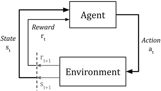
FIGURE 1. Top-level view of the interaction between the Agent and the Environment.

The RL problem can be modelled by a finite Markov Decision Process (MDP) which is defined by a (s_t, a_t, r_t, s_t+1) tuple. A set of tuples of size H constitute an episode, where the initial state is drawn from the initial state distribution, s₀ ∼ p₀. The reward is a scalar representing the goodness of the last action performed on the environment. The ultimate goal of any RL algorithm is to maximise the expected discounted cumulative future reward, or return (G), obtained by the agent:

$G_t\triangleq {\mathbb{E}}_{a\sim {\pi }_{\theta },s\sim p\left(s_{t+1}|s_t,a_t\right)}\sum _{i=t}^{H-t}{\gamma }^{i}r\left(s_i,a_i\right)$

where π_θ is known as the policy, which maps the states to the actions and is parameterised by vector θ. p (s_t+1|s_t, a_t) is the transition distribution of the environment. γ is called the discount factor (γ ≤ 1, e.g., 0.99) and its role is to control the importance of future rewards in the calculation of the value for a particular state. RL nomenclature defines the value function as a measure of the total expected future rewards the agent can expect when starting in some state, s [5].

Figure 2 shows a non-exhaustive taxonomy of the various RL algorithms found in the literature. RL can be split into two main classes: Model-Free (MF) and Model-Based (MB) algorithms. As the name implies, MF RL is the study of algorithms that do not require a model to be learned and solely depend on the relationship among the actions, states and rewards obtained on every interaction. On the other hand, MB RL is the study of algorithms that either has access to the full dynamics model, e.g., AlphaGo [6], or require that a model of the environment is learned alongside the agent, e.g., Model-Ensemble Trust-Region Policy Optimization (ME-TRPO) [7].

FIGURE 2

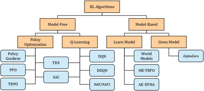
FIGURE 2. A non-exhaustive taxonomy of RL algorithms.

The first RL algorithm considered in this work is Normalized Advantage Functions (NAF), which was introduced in [8] and is based on Deep Q Networks (DQN) and Duelling DQN (DDQN) to solve continuous tasks, e.g., robotic arm control. These types of algorithms update a policy that did not necessarily create the trajectory; hence they are called off-policy methods.

Unlike DQN, NAF contains a network with three output streams: 1) Value function estimate, $\widehat{V}(s)$; 2) Advantage estimate $\widehat{A}(s,a)$; 3) Policy μ(s), where:

$Q\left(s,a;\theta \right)\triangleq V\left(s;\theta \right)+A\left(s,a;\theta \right)(1)$

By taking the argmax over the actions in the Advantage, the agent learns the optimal Q-value. NAF differs from standard Q-learning methods since A is explicitly parameterised as a quadratic function of non-linear features of the state:

$\begin{array}{ll}\hfill A\left(s,a;\theta \right)& =-\frac{1}{2}{\left(a-\mu \left(s;\theta \right)\right)}^{⊺}P\left(s;\theta \right)\left(a-\mu \left(s;\theta \right)\right)\hfill \\ \hfill P\left(s,\theta \right)& \triangleq L\left(s;\theta \right)L{\left(s;\theta \right)}^{⊺}\hfill \end{array}(2)$

where L is a lower-triangular matrix with an exponentiated diagonal, constructed from the second output stream of the network. By Eq. 2, p is a state-dependent, positive-definite square matrix. The third output stream of the network is μ(s; θ), which is the action that maximises the Q-function in Eq. 1 when the following loss is minimised:

$\mathcal{L}=\frac{1}{N}\sum _i{\left(y_i-Q\left(s_i,a_i;\theta \right)\right)}^2$

with:

$y_i=r_i+\gamma V^{\prime }\left(s_{i+1};{\theta }^{\prime }\right)$

V′(⋅; θ′) denotes the target network which is a separate network, updated slower than the main network, V (⋅; θ) by using Polyak averaging on their parameters:

${\theta }^{\prime }\leftarrow \tau \theta +\left(1-\tau \right){\theta }^{\prime }$

where τ is set to a small number, e.g., 0.005. Hirlaender et al. introduced NAF2 in [9], which adds clipped smoothing noise to the actions, a technique also used in the Twin-Delayed Deep Deterministic Policy Gradient (TD3) algorithm to stabilise the policy training [10].

The second algorithm is Proximal Policy Optimization (PPO) introduced in [11], which is primarily based on the Policy Gradient (PG) method. PG methods use trajectory rollouts created by taking actions from the most recent policy trained by the agent on the environment; hence they are called on-policy methods. The most common form of the PG objective is written as:

${\mathcal{J}}^{PG}\left(\theta \right)={\widehat{\mathbb{E}}}_{t,a_t\sim {\pi }_{\theta }\left(s_t\right),s_{t+1}\sim p\left(\cdot |s_t,a_t\right)}\left[\log {\pi }_{\theta }\left(a_t|s_t\right){\widehat{A}}_t\right]$

The expectation symbol $\widehat{\mathbb{E}}$ denotes the empirical average over a batch of rollouts denoted by t, actions a_t sampled from π_θ(⋅), which is a stochastic policy. ${\widehat{A}}_t$ is an estimate of the Advantage, which is a measure of how good a_t is compared to the average action possible at time t. Differentiating ${\mathcal{J}}^{PG}$ with respect to the network parameters, θ, obtains the PG estimate, $\widehat{g}$:

$\widehat{g}={\widehat{\mathbb{E}}}_t\left[{▿}_{\theta }\log {\pi }_{\theta }\left(a_t|s_t\right){\widehat{A}}_t\right]$

The gradient estimate is used in gradient ascent to maximise the objective ${\mathcal{J}}^{PG}$. It was also shown in [11] that performing multiple optimisation steps using the same trajectory leads to destructively large policy updates that no longer converge to an optimal policy. Trust Region Policy Optimization (TRPO) introduced a solution by constraining the maximisation of ${\mathcal{J}}^{PG}$ by:

${\widehat{\mathbb{E}}}_t\left[D_{KL}\left[{\pi }_{{\theta }_{\mathit{old}}}\left(\cdot |s_t\right),{\pi }_{\theta }\left(\cdot |s_t\right)\right]\right]\le \sigma (3)$

where $\sigma \in \mathbb{R}$, e.g., 0.01, θ_old is the policy parameters before the policy update and θ after the update. One drawback of TRPO is its implementation complexity. PPO uses a similar approach to TRPO, however, instead of constraining the policy to satisfy Eq. 3, PPO introduces a clipped policy objective with a penalty proportional to the KL-divergence between the old and new policy:

$r_t\triangleq \frac{{\pi }_{\theta }}{{\pi }_{{\theta }_{\mathit{old}}}}(4)$

$\begin{array}{ll}\hfill & {\mathcal{J}}^{\mathit{CLIP}}\left(\theta \right)=\hfill \\ \hfill {\widehat{\mathbb{E}}}_t& \left[\text{min}\left(r_t\left(\theta \right){\widehat{A}}_t,\text{clip}\left(r_t\left(\theta \right),1-ϵ,1+ϵ\right){\widehat{A}}_t\right)\right]\hfill \end{array}(5)$

${\mathcal{J}}^{\mathit{CLIP}}$ is easier to implement and executes faster than TRPO. Experiments done in [11] also show that PPO and TRPO obtain a similar performance over many types of environments¹.

The most noticeable difference between off-policy and on-policy methods mentioned so far is the two types of policies used; deterministic and stochastic, respectively. NAF2 has a deterministic policy, which means that the agent will always choose the same action for one state. For each state, the stochastic policy of PPO provides an action distribution that can be sampled for the next action².

More RL algorithms were attempted, and their training and evaluation can be found in the Supplementary Material. The Soft Actor-Critic (SAC) algorithm combines the use of stochastic policies and the off-policy method by introducing the concept of entropy maximisation to RL [12]. Anchored-Ensemble DYNA-style (AE-DYNA) is an MBRL algorithm that internally relies on a SAC agent to optimise a policy in an uncertainty-aware world model [9].

3 Environment

The QFB uses two Q_RM per beam and each Q_RM is set up by default to contain six outputs: the horizontal and vertical tune, the horizontal and vertical chromaticity, and the real and imaginary components of the coupling coefficient. To separate the QFB from the coupling and chromaticity control, the Q_RM is truncated to have only two outputs; the tunes. The tune control sequence occurs at 12.5 Hz and a predefined sequence of steps is performed where: 1) the tune error, $\mathrm{\Delta }\vec{Q}$, is obtained by subtracting the current tune estimate and the reference tune; 2) the tune error is clipped to $\approx 56\text{Hz}$¹; 3) a velocity form Proportional-Integral (PI) controller is applied by using $\mathrm{\Delta }\overrightarrow{Q_t}$ and $\mathrm{\Delta }\overrightarrow{Q_{t-1}}$, where t denotes the time step; 4) the PI output is multiplied by the pseudo-inverse matrix of Q_RM (Tune Pseudo-Inverse (Q_PI) computed by Singular Value Decomposition) to obtain a set of residual quadrupole currents; 5) the currents are multiplied by -1; 6) the currents are globally scaled by a factor k ≤ 1 to accommodate the slew rate of the quadrupoles; 7) finally the corrections are sent to the quadrupole power converters via UDP packets.

An OpenAI Gym environment [13] was set up to mimic the response of the LHC to a varying quadrupolar magnetic field. This environment will hereon be referred to as QFBEnv. QFBEnv has two continuous states as output and uses 16 bounded continuous actions as input. The states and actions were normalised to the range [ − 1, 1]. The normalised state-space represented a range of [−25 Hz, 25 Hz] of tune error.

QFBEnv implicitly implemented current slew rate limiting since the actions were clipped to the range [-1,1]. A saturated action in QFBEnv is the maximum change in a quadrupolar field strength that the magnets can supply in the next time step. The normalised action space represented the fraction of the total allowable current rate in the magnets. Every step was also assumed to occur every 80 ms, which corresponds to the QFB controller frequency of 12.5 Hz. Therefore a normalised action of one on a magnet with a maximum current rate of 0.5 A s⁻¹ is equivalent to a current change of 0.5 × 0.08 = 40 mA.

In addition, the PI controller used by the QFB was also re-implemented as a particular method within QFBEnv. This was done to provide a reference for the performance of a trained agent. The proportional, K_p, and integral, K_i, gains of the PI controller were set to low values by default as a conservative measure during initialisation of the QFB. To ensure a fair comparison, the PI controller was tuned using the Ziegler-Nichols method [14]: 1) K_i was set to zero; 2) K_p was increased until state oscillations were observed; 3) the latest value of K_p was halved; 4) K_i was increased until state oscillations were observed; 5) K_i was halved. The final gains for the PI controller implemented in QFBEnv were K_p = 1,000 and K_i = 2000.

The PI controller was implemented with the global slew rate limiting. As an example, consider a quadrupole magnet, M, with a slew rate of 0.5 A s⁻¹. If a current change at 1 A s⁻¹ is requested for the next time step, all of the outputs of the PI controller are scaled by a factor k = 0.5 to accommodate M. The global factor k can be decreased if another magnet requires k < 0.5 to accommodate its respective slew rate. QFBEnv does not enforce the global scaling scheme by default, therefore any action within the [ − 1, 1] bounds are applied to the environment within the next time step.

QFBEnv implemented two important functionalities: 1) the reset function and; 2) the step function. The reset function is the entry point to a new episode, whereby a new initial state, (ΔQ_Hor.,0, ΔQ_Ver.,0), is generated and returned to the agent. The step function is responsible for accepting an action, following the transition dynamics of the environment and then returning a tuple containing: 1) the next state; 2) the reward and; 3) a Boolean flag to indicate episode termination. The reward was chosen to be the negative average quadratic of the state, as shown in Eq. 6.

$r_{t+1}=-\frac{1}{n}\sum _i^n{\left(s_{t+1}^{\left(i\right)}\right)}^2(6)$

Since the goal of any RL agent is to maximise the reward, a perfectly trained agent would thus have a policy which reduces the tune error to zero. It is also important to note that the gradient of quadratic reward increases, the farther the state is from the optimal point. This reflects the importance of controlling a larger tune error with respect to a smaller error in the QFB, e.g., if ΔQ_H ≫ΔQ_V > Goal, the agent would put more importance on the correction of ΔQ_H. From trial and error, this shape of reward was observed to produce more stable training.

An episode is defined as starting from the first state initialisation until a terminal state is reached. A baseline optimal episode length was obtained by running 1,000 episodes using the PI controller. The measured average optimal episode length was $\approx 28\pm 6$ steps. The maximum allowable episode length in QFBEnv was chosen to be 70 steps long, approximately double the maximum optimal episode length observed. Successful early termination in QFBEnv is defined as the latest five rewards being above a threshold. The threshold value of QFBEnv was chosen as a maximum tune error in both planes of 1 Hz. This is equivalent to $\frac{1}{25}=0.04$ in normalised state space and the threshold reward can be obtained from Eq. 6:

$r_{\mathit{thresh}}=-\frac{1}{2}\left(0.04^2+0.04^2\right)=-0.0016$

Thus, a terminal state could be reached either by a successful early termination or after 70 steps were made without success. The successful early termination represents a real operational scenario, since the QFB is typically switched off manually when the measured tunes are close to their respective reference values. It also allows for more examples of the state below the threshold to be experienced by the RL agents, which leads to better learning close to the threshold boundary.

4 Training

Table 1 tabulates information about the types of RL algorithms which were trained on QFBEnv. The two algorithms which obtained the best performing policies were NAF2 and PPO. The training process of SAC, TD3 and AE-DYNA can be found in the Supplementary Material.

TABLE 1

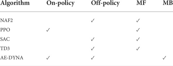
TABLE 1. The RL algorithms attempted in this work along with their type of policies and whether they train a world model: Model-Free (MF) or Model-Based (MB).

During the training of the Model-Free (MF) agents, two callback functions were used: Callback A was called every 1,000 training steps to save the network parameters of the most recent agents to disk and; Callback B was called every 100 training steps to evaluate and log the performance of the most recent agent. The performance of the most recent agent was evaluated on a separate instance of QFBEnv in Callback B. Twenty episodes were played in sequence using the most recent agent to choose the actions. The training metrics were the average episode length, average undiscounted episode return and the average success rate. These values were logged with Tensorboard [15] and are used in the remaining part of this section to describe the training process of each algorithm.

SAC and TD3 required the most hyperparameter tuning to obtain a satisfactory result. NAF2 and PPO were less susceptible to hyperparameter tuning. AE-DYNA was more complex to set up correctly and also required some network adjustments in order for it to learn a successful policy on QFBEnv. The evolution of the agent throughout the training process was analysed off-line and the various policies trained by the different RL algorithms were re-loaded and compared.

All the agents used the same network architecture for their policies. The final architecture was chosen through a grid-search as an artificial Neural Network (NN) with two hidden layers having 50 nodes each and using the Rectified Linear Unit (ReLU) activation function. This network architecture was also used for the value function networks of the off-policy agents.

In on-line training on the QFB, the worst case episode length is 70 steps and every step is taken at a rate of 12.5 Hz. Therefore the maximum time of one episode on the QFB is:

$\frac{70\text{steps}}{12.5\text{Hz}}=5.6\text{s}.(7)$

At episode termination, the actuators controlled by the action of the agent would, at worst, need to be re-adjusted to their initial settings at the start of the episode, e.g. set to reference current. The worst-case scenario occurs when an action is saturated throughout the episodes. The worst-case re-adjustment time for one episode is thus equal to Eq. 7, 5.6s. Each RL algorithm trained in this work is attempted five times with different random seeds. An estimate of the real on-line training time on the LHC is also provided, which considers the worst case re-adjustment time for all the actuators. To achieve this, all training time estimates obtained from off-line environments were doubled to obtain the worst-case training time in an on-line environment.

Table 2 tabulates the hyperparameters that obtained the best NAF2 agent in this work. The discount factor, γ and the time constant for the Polyak averaging of the main and target networks, τ were set to the values listed in [9]. q_σ set up the standard deviation of the action smoothing noise applied at each step in QFBEnv when acquiring data. q_clip clipped the action smoothing noise to a range [ − q_clip, q_clip]. q_σ and q_clip were chosen by trial and error. In addition to the smoothing noise, a decaying action noise was also applied during training. The following noise function was used:

$a_i≔a_i+\mathcal{N}\left(\mathrm{0,1}\right)\times \text{max}\left(1-\frac{{\text{ep}}_{\mathit{idx}}}{40},0\right)$

where a_i denotes the i^th action, $\mathcal{N}(\mathrm{0,1})$ is a standard Gaussian, and ep_idx is current episode number. Therefore, the action noise decays linearly to zero after 40 episodes. Note that the choice to decay the action noise relative to the number of episodes was arbitrary. The action noise can be made to decay relative to the number of steps taken so far during training.

TABLE 2

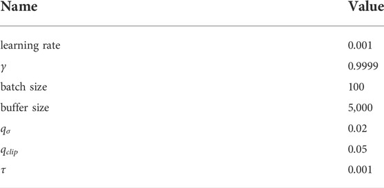
TABLE 2. Hyperparameters used for NAF2.

Figure 3 shows the training performance statistics of the NAF2 agents. Figure 3A shows that the episode length decreases below 20 after 20000 steps. Figure 3C shows that the success rate goes to 100% after 20000 steps as well. From Figure 3B it can be seen that the average undiscounted return of the NAF2 agents was higher at the end of training. This shows a monotonic improvement in performance, regardless of the Min-Max bounds of NAF2 shown in Figures 3A,C. Partially solved episodes explain the large Min-Max boundaries. The policy manages to increase the reward in these episodes until a local minimum is reached without satisfying the successful early termination criterion. However, slight improvements in the policy push the states closer to the threshold, subsequently increasing the return.

FIGURE 3

FIGURE 3. Performance statistics of NAF2 and PPO agents during training. The hyperparameters used are tabulated in Table 2 and Table 3, respectively. (A) Median episode length; (B) Median undiscounted episode return and; (C) Median success rate, of five agents initialised with different random seeds, per algorithm.

Successful policies using NAF2 were relatively sample-efficient to train when compared to other algorithms attempted. The monotonic improvement shown in Figure 3B implies that a successful agent can be expected relatively early in terms of training steps taken on the environment. Some agents during the training performed well, with an average episode length of 20 steps after approximately 20,000 steps. In real LHC operation on the QFB, the worst-case training time of 20,000 steps is calculated by:

$\frac{\mathrm{20,000}\text{steps}}{12.5\text{Hz}}\times 2\approx 53\text{min}$

The hyperparameters shown in Table 3 are the salient parameters of the Proximal Policy Optimization (PPO) algorithm as implemented in Stable Baselines. Note that ϵ is the clipping parameter from Eq. 5. PPO proved to be the easiest algorithm to apply to QFBEnv in terms of hyperparameter tuning and usage. Figure 3A shows that PPO converges below an episode length of 20 after around 20000 training steps. A solution that drops the episode length to below ten steps is found after approximately 40000 steps. This remains stable until catastrophic forgetting of the policy occurs after 80000 steps. Figure 3C also shows that some agents expected a 100% success rate between 20000 and 80000 steps. Figure 3B illustrates that the episode return for PPO is not guaranteed to be monotonically improving. The best median performance of PPO was reached at approximately 86000 steps and obtained an undiscounted episode return of -4. All the metrics in Figure 3 shows that the PPO performance starts to degrade beyond this training step.

TABLE 3

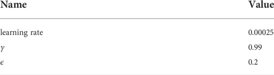
TABLE 3. Hyperparameters used for PPO.

The catastrophic forgetting of the policy, however, did not occur quickly. At around 90000 steps, the expected episode length had increased to 20 steps again. A callback function can easily halt training if the policy starts forgetting and freezing the network parameters to obtain the best performing agent. This predictability is essential if the agent training occurs in the real LHC operation. Similarly to NAF2, approximately 20000 steps are required to learn a good policy which is equivalent to a worst-case on-line training time of 53 min.

5 Evaluation

This section evaluates the behaviour of the best policies obtained by each RL algorithm in corner cases of QFBEnv. These evaluations were performed by loading the network parameters of the agent with the best performance and recording its interactions with QFBEnv over multiple episodes. To ensure a fair comparison, a reference trajectory was created for each episode by using the actions from the PI controller and the same initial state. The PI controller was also subjected to the same tests, e.g., Gaussian noise was added to the action calculated by the PI controller in Figure 4B.

FIGURE 4

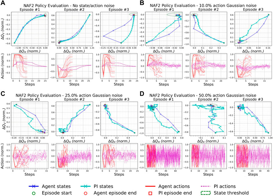
FIGURE 4. Episodes from the best NAF2 agent and the PI controller with the same initial states and with a varying additive Gaussian action noise with zero mean and standard deviation as a percentage of the half action space [0, 1]. (A) 0%, (B) 10%, (C) 25%, and (D) 50% Gaussian action noise.

5.1 Effect of Gaussian noise

QFBEnv implements a deterministic model and actions passed through the step function are deterministic by default. However, by adding Gaussian noise to the action chosen by the policy, stochasticity can be introduced externally to QFBEnv. By subjecting each agent to a stochastic environment, the general robustness of each agent can be empirically verified. During this test, the initial state per episode was ensured to be sufficiently randomised to show more coverage of the state-action space.

The evolution of the episode trajectories are shown in sets of three evaluation episodes, e.g., Figure 4A. The state plots correspond to the evolution of ΔQ_H and ΔQ_V in time of the RL agents (top blue plots) and PI controller (top cyan plots), respectively. Green and red markers denote the start and end of each episode, respectively. A boundary (dashed green ellipse) is also drawn to indicate the success threshold state. The action plots correspond to the evolution of the 16 actions in time of the RL agents (bottom red plots) and PI controller (bottom magenta plots), respectively, until a terminal state is reached. Each set is obtained by applying Gaussian action noise with a zero mean and a standard deviation equal to 10%, 25%, and 50% of half the action range ([0,1]), respectively.

Figure 4A shows three episodes obtained with a deterministic NAF2 policy where it converges to an optimal state in approximately ten steps, while the PI controller takes approximately 25 steps until successful termination. However, it can be seen that the action chosen by the NAF2 policy at each terminal state is a non-zero vector. Ideally, the magnitudes of the actions are inversely proportional to the reward in Eq. 6, e.g., the PI actions of Figure 4A. This implies that NAF2 converged to a sub-optimal policy. Figures 4B–D show that the NAF2 policy satisfies the early termination criterion in each episode. The longest episode can be observed in Figure 4D to be approximately 20 steps long. Moreover, Episode #1 of Figure 4D shows that the PI controller failed to satisfy the successful early termination criterion. This indicates that the best agent trained by NAF2 performs better than the PI controller in a stochastic QFBEnv.

Figure 5A shows three episodes obtained by applying the actions sampled from the PPO stochastic policy, deterministically to QFBEnv, i.e., no noise applied. Similarly to NAF2, PPO converges to the optimal state. Furthermore, the actions of PPO start to converge back to zero at the end of the episode, which implies that PPO learned an optimal policy. Figures 5B–D show that the agent satisfies the early termination criterion in each scenario. PPO also shows a wider range of episode lengths as the action noise is increased; the episode lengths in Figure 5D vary more than for NAF2 in Figure 4D. Therefore, this test indicates that the policy obtained by NAF2 is slightly more robust to action noise than PPO.

FIGURE 5

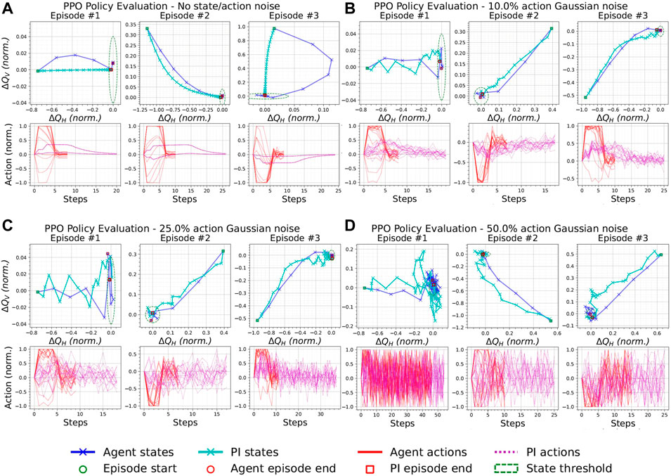
FIGURE 5. Episodes from the best PPO agent and the PI controller with the same initial states and with a varying additive Gaussian action noise with zero mean and standard deviation as a percentage of the half action space [0, 1]. (A) 0%, (B) 10%, (C) 25%, and (D) 50% Gaussian action noise.

The action noise was also varied with a finer interval to aid with the analysis of the best agents under its effect and more statistics were taken on the performance of the agents and the PI controller e.g., Figure 6A. For each action noise value on the x-axis, 1,000 episodes were executed and used to obtain the statistics shown in the respective figures. These plots illustrate more information on the distribution of key measurements linked with the performance of the agents (in blue) and the PI controller (in red). In particular, the distributions of the following measurements are presented: 1) Episode length (one scalar per episode); 2) Distance of the terminal state from the optimal state of [ΔQ_H = 0, ΔQ_V = 0], calculated by Eq. 8 and is referred to as Distance To Optimal (DTO) (one scalar per episode);

$\text{DTO}=\sqrt{\mathrm{\Delta }{Q}_H^2+\mathrm{\Delta }{Q}_V^2}(8)$

and c) Concatenated values of the last actions applied in the episode before termination, be it successful or otherwise (array of size 16 per episode).

FIGURE 6

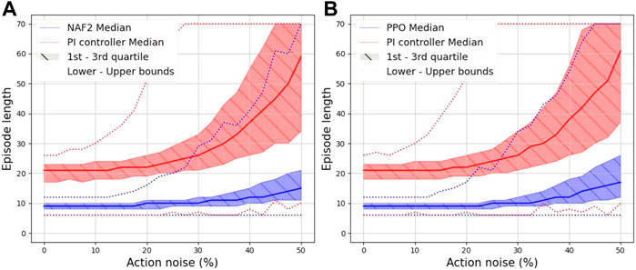
FIGURE 6. Effect of action noise on the episode length due to varying action noise on (A) the best NAF2 agent, (B) the best PPO agent and the PI controller.

Table 4 tabulates the episode length statistics collected from 1,000 episodes, for the values of Gaussian action noise considered in the episode evaluation plots. As illustrated in Figure 6, the mean and the standard deviation of the episode lengths obtained by the NAF2 agent in Figure 6A and by the PPO agent in Figure 6B, outperformed those of the PI controller. Furthermore, the upper bound of the PI controller episode lengths reaches 70 steps at approximately 25% action noise; this indicates that the PI controller starts to fail to successfully terminate episodes at this point. This corresponds with the results shown in Figure 7 where at approximately 25% action noise, the upper bound of the DTO of the PI controller moves past the Goal threshold set within the QFBEnv (green dashed line). Both the NAF2 agent in Figure 7A and the PPO agent in Figure 7B maintain an upper bound DTO below the threshold until approximately 45% action noise.

TABLE 4

TABLE 4. The statistics (mean ± std.) for the episode length obtained by the best RL agents trained in Section 4 and PI controller with respect to the amplitude of Gaussian action noise.

FIGURE 7

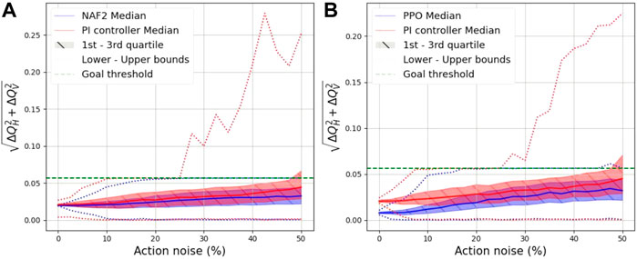
FIGURE 7. Effect of action noise on the distance to the optimal point at the end of the episode due to varying action noise on (A) the best NAF2 agent, (A) the best PPO agent and the PI controller.

Figure 8 illustrates the statistics of the last action chosen in each episode. Figure 8A exposes the weakness of the NAF2 agent, where it can be observed that the values of the last actions are unpredictable even without action noise, i.e., at 0% action noise, the PI controller actions are below ±0.05 while the NAF2 action value distribution populates most of the action range. These results signify that NAF2 has trained a policy which outperforms the PI controller in a noisy environment, albeit the policy is sub-optimal.

FIGURE 8

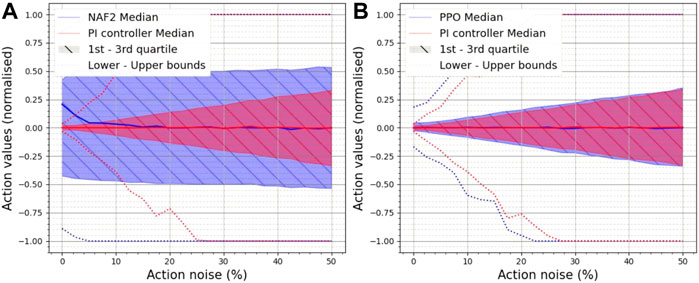
FIGURE 8. Effect of action noise on the last action used in the episode due to varying action noise on (A) the best NAF2 agent, (B) the best PPO agent and the PI controller.

Figure 8B illustrates that the PPO policy chooses last actions which behave similarly to the PI controller in the presence of Gaussian action noise. At 0% action noise, the distribution of the PPO last action values are slightly larger than those of the PI controller. However, as the action noise is increased the distribution widths of both PPO and the PI controller increase at the same rate. This consolidates what was observed in Figure 5, where the last action values are dispersed with respect to the amplitude of the action noise applied. This concludes that PPO successfully trained a policy on QFBEnv which is also the closest to the optimal policy. LATEX.

5.2 Effect of actuator failure

In this test, the performance of the best policies trained in this work was analysed in the presence of magnet failures. For each episode shown in this section, an action was chosen at random at a predetermined step in the episode. For the remaining steps until a terminal state, the action chosen was set to -1 to simulate a cool-down of the magnet after a circuit failure. The corresponding action obtained by the PI controller was set to the same value. While this test is not a perfect representation of magnet failures in the LHC, it is a worst-case scenario that tests the performance of the policies and PI controller in unseen and unideal conditions.

For each policy, two scenarios with three episodes each are shown. In the first scenario, one actuator fails on step 1; in the second scenario, three actuators fail on steps 1, 2, and 3, respectively. All the plots shown in this test also show an episode trajectory obtained by repeating the episode with the same initial conditions and all actions functioning. The episode trajectories affected by the actuator failures use × as a marker, while the episodes using all actions use ▴ as a marker. It was also found that a maximum episode length of 70 obtained large state deviations for certain scenarios. To aid the analysis of the results, the maximum episode length was set to 20.

The evaluation episodes from the best NAF2 agent with one actuator failure are shown in Figure 9A. It can be observed that the PI controller already diverges from the threshold boundary and fails on all episodes. NAF2 succeeds in terminating $\frac{1}{3}$ of the episodes in under 20 steps. At three actuator failures in Figure 9B, the terminal state achieved by NAF2 is within four times the value of the threshold, while the PI controller terminal state shifts farther from the optimal point.³

FIGURE 9

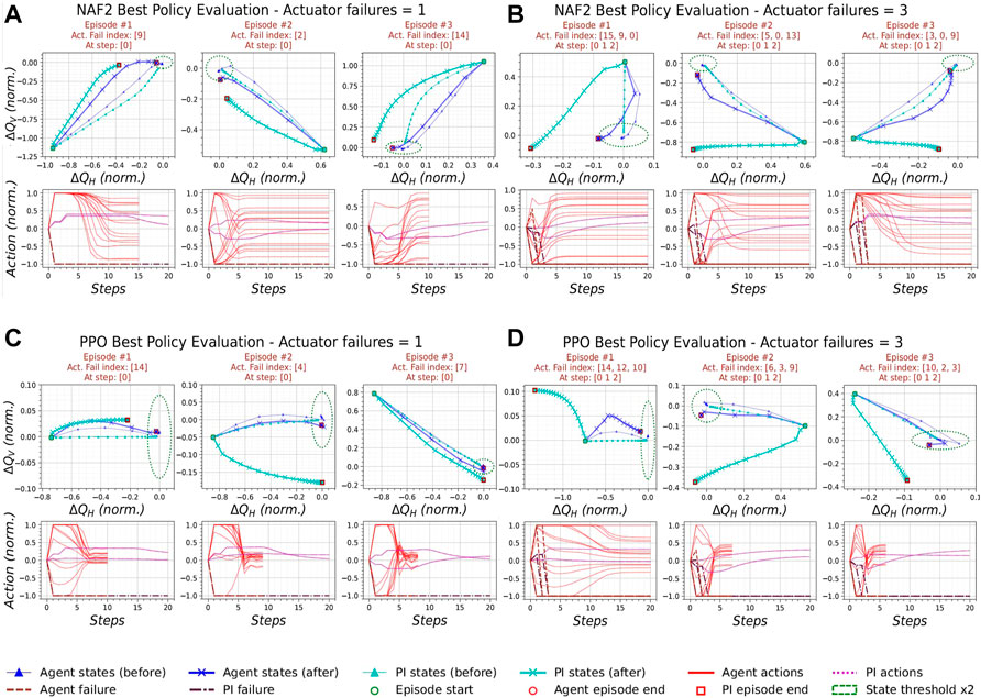
FIGURE 9. Episodes from the best RL agents and the PI controller under the effect of different number of actuator failures.(A) NAF2 agent with one actuator failure, (B) NAF2 with three actuator failures, (C) PPO agent with one actuator failure, (D) PPO agent with three actuator failures.

Similarly to NAF2, PPO performs better than the PI controller in all scenarios of actuator failures in Figure 9C and Figure 9D. The effect of an increasing number of actuator failures on the best PPO policy is also evident in the action plots of the PPO actuator failure tests. These figures, along with bottom plots of Figure 5A, show that when all actions are used, the actions decay the closest to zero at the end of the episode. They also show that the actions still decay during actuator failures. However, the actions remain separated by a range proportional to the number of actuators that failed during the episode. This observation suggests that the PPO policy has successfully generalised the optimal policy trained on one environment to another environment with slightly different model dynamics.

5.3 Effect of incorrect tune estimation

This test subjects the best agents to the effects of 50 Hz noise harmonics on the BBQ system. A similar procedure to the previous test is followed, where the best agent trained by each respective RL algorithm is loaded and is used to produce evaluation episodes. The only difference in this test is that after each step in the environment, the state is intercepted and a perturbation is added, which simulates the effect of 50 Hz noise harmonic-induced perturbations within the state.

These perturbations were obtained by the following steps: 1) The state, ΔQ, was added to a random frequency, f_r²; 2) The realistic second-order system spectrum simulation procedure in [16] was performed for a spectrum with a resonance frequency, $f_{\mathit{res}}^{\mathit{true}}=f_r+\mathrm{\Delta }Q$ and damping factor $\zeta \sim 10^{\mathcal{U}(-2.5,-1.8)}$³; 3) The BQ algorithm is used to obtain perturbed tune estimates [16]. All the plots shown in this section also show black dashed lines which mark the locations of the horizontal and vertical 50 Hz harmonics in normalised state space.

Figure 10 and Figure 11 show three episodes obtained by the best NAF2 and PPO policies, respectively, when the state is perturbed by 50 Hz noise harmonics. It can be observed that the states of the policies (dark blue) appear to be concentrated around an intersection of a horizontal and vertical 50 Hz noise harmonics, which is closest to the optimal point of the state space. On the other hand, the PI controller states sometimes extend up to three 50 Hz harmonics from the optimal point. This observation suggests that even without the tune estimation renovation discussed in [16, 17], it is possible to train NAF2 and PPO agents to maintain the tune error as close as possible to the optimal point.

FIGURE 10

FIGURE 10. Effect of inaccurate tune estimation on the best NAF2 agent.

FIGURE 11

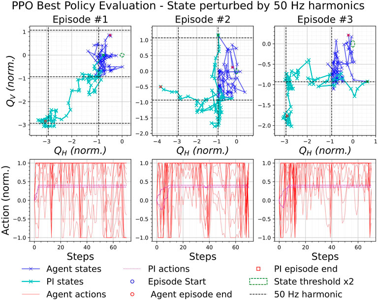
FIGURE 11. Effect of inaccurate tune estimation on the best PPO agent.

5.4 Summary

When taking into consideration the algorithms shown in the Supplementary Material, NAF2 and PPO trained the best two policies. However, AE-DYNA-SAC was the most sample efficient and also obtained a policy that is stable in low action noise. The policies trained by TD3 and SAC were sometimes successful. However, their performance was significantly worse than NAF2 and PPO. On the other hand, the best SAC-TFL agent trained an adequate policy that works well on QFBEnv.

6 Conclusion and future work

This work explored the potential use of RL on one of the LHC beam-based feedback controller sub-systems, the QFB. An RL environment called QFBEnv was designed to mimic the QFB in real operation in the LHC. The original implementation of the QFB PI controller was re-implemented to serve as a reference agent to the trained RL agents.

A total of five RL algorithms were selected from literature and trained on QFBEnv. A series of evaluation tests were performed to assess the performance of the best two agents against the standard controller paradigm. These tests were designed to capture the performance of the agents during corner cases. PPO and NAF2 obtained a high performance in each test. Slightly better generalisation was also observed during the actuator failure tests. The training and evaluation of the other RL algorithms attempted in this work are in the Supplementary Material. It was not easy to tune the hyperparameters of TD3 even in the most straightforward deterministic cases, while depending on the implementation, the SAC algorithm could learn a good policy. Finally, AE-DYNA-SAC was the most sample efficient agent attempted, and the performance of the best policy trained was comparable to that of the PI controller.

Our studies showed that RL agents could generalise the environment dynamics and outperform the standard control paradigm in specific situations which commonly occur during accelerator operation.

Future work will concentrate on more sample efficient RL algorithms, e.g., Model-Based Policy Optimization (MBPO) [18] since the real operation is restricted by the beam time. By addressing robustness and sample efficiency when training on simulations, it will be possible to design an RL agent that can be feasibly trained on the QFB during the LHC Run 3. As was shown in this work, this would allow for more reliable tune control even in situations where the standard controller is not applicable.

Data availability statement

The raw data supporting the conclusions of this article will be made available by the authors, without undue reservation.

Author contributions

LG and GV contributed to the conception and design of the study. LG contributed to the implementation, logging and plotting of results. All authors contributed to the manuscript revision.

Funding

Project DeepREL financed by the Malta Council for Science and Technology, for and on behalf of the Foundation for Science and Technology, through the FUSION: R&I Research Excellence Programme.

Conflict of interest

The authors declare that the research was conducted in the absence of any commercial or financial relationships that could be construed as a potential conflict of interest.

Publisher’s note

All claims expressed in this article are solely those of the authors and do not necessarily represent those of their affiliated organizations, or those of the publisher, the editors and the reviewers. Any product that may be evaluated in this article, or claim that may be made by its manufacturer, is not guaranteed or endorsed by the publisher.

Supplementary material

The Supplementary Material for this article can be found online at: https://www.frontiersin.org/articles/10.3389/fphy.2022.929064/full#supplementary-material

Footnotes

¹As implemented in the QFB; $0.01\times \frac{F_s}{2}$ where the sampling frequency, F_s, of the BBQ system is equal to the LHC revolution frequency, 11 245.55 Hz.

²Initialised randomly and set constant throughout one episode.

³$\mathcal{U}$ is a uniform distribution.

References

1. Steinhagen RJ. LHC beam stability and feedback control-orbit and energy. Ph.D. thesis. Aachen, Germany: RWTH Aachen U (2007).

2. Grech L, Valentino G, Alves D, Calia A, Hostettler M, Wenninger J, Jackson S. Proceedings of the 18th international conference on accelerator and large experimental Physics control systems (ICALEPCS 2021) (2021).

Google Scholar

3. Gasior M, Jones R. Proceedings of 7th European workshop on beam diagnostics and instrumentation for particle accelerators (DIPAC 2005) (2005). p. 4.

Google Scholar

4.MAD - methodical accelerator design (2019). p. 2019–626. Accessed.

Google Scholar

5. Sutton RS, Barto AG. Reinforcement learning - an introduction, adaptive computation and machine learning. Cambridge, MA, USA: The MIT Press (2018).

Google Scholar

6. Silver D, Huang A, Maddison CJ, Guez A, Sifre L, van den Driessche G, et al. Mastering the game of Go with deep neural networks and tree search. Nature (2016) 529:484–9. doi:10.1038/nature16961

PubMed Abstract | CrossRef Full Text | Google Scholar

7. Kurutach T, Clavera I, Duan Y, Tamar A, Abbeel P. Model-Ensemble Trust-Region policy optimization (2018). arXiv:1802.10592 [cs.LG].

Google Scholar

8. Gu S, Lillicrap T, Sutskever I, Levine S. International conference on machine learning (2016). p. 2829–38.

Google Scholar

9. Hirlaender S, Bruchon N. Model-free and bayesian ensembling model-based deep reinforcement learning for particle accelerator control demonstrated on the FERMI FEL (2020). arXiv:2012.09737 [cs.LG].

Google Scholar

10. Fujimoto S, van Hoof H, Meger D. Addressing function approximation error in Actor-Critic methods (2018). arXiv:1802.09477 [cs.AI].

Google Scholar

11. Schulman J, Wolski F, Dhariwal P, Radford A, Klimov O. Proximal policy optimization algorithms (2017). arXiv:1707.06347 [cs.LG].

Google Scholar

12. Haarnoja T, Zhou A, Abbeel P, Levine S. Soft Actor-Critic: Off-Policy maximum entropy deep reinforcement learning with a stochastic actor (2018). arXiv:1801.01290 [cs.LG].

Google Scholar

13. Brockman G, Cheung V, Pettersson L, Schneider J, Schulman J, Tang J, et al. Openai gym (2016) 1606:01540.

14. Ziegler JG, Nichols NB. J Dyn Syst Meas Control (1942) 115:220.

15. Abadi M, Barham P, Chen J, Chen Z, Davis A, Dean J, et al. 12th USENIX symposium on operating systems design and implementation (OSDI 16). Savannah, GA: USENIX Association (2016). p. 265–83.

Google Scholar

16. Grech L, Valentino G, Alves D, Gasior M, Jackson S, Jones R, et al. Proceedings of the 9th international beam instrumentation conference (IBIC 2020 (2020).

Google Scholar

17. Grech L, Valentino G, Alves D. A machine learning approach for the tune estimation in the LHC. Information (2021) 12:197. doi:10.3390/info12050197

CrossRef Full Text | Google Scholar

18. Janner M, Fu J, Zhang M, Levine S. In: H Wallach, H Larochelle, A Beygelzimer, F d Alché-Buc, E Fox, and R Garnett, editors. Advances in neural information processing systems, Vol. 32. Red Hook, NY, USA: Curran Associates, Inc. (2019).

Google Scholar

19. Achiam J. Spinning up in deep reinforcement learning (2018).

Google Scholar

20. Dhariwal P, Hesse C, Klimov O, Nichol A, Plappert M, Radford A, et al. Openai baselines (2017).

Google Scholar

21. Hill A, Raffin A, Ernestus M, Gleave A, Kanervisto A, Traore R, et al. Stable baselines (2018). Available from: https://github.com/hill-a/stable-baselines (Accessed Septermber, 2021).

Google Scholar

22. Hirländer S. MathPhysSim/FERMI_RL_Paper. Preprint release (2020).

Google Scholar

23.Addressing function approximation error in actor-critic methods (2018). arXiv:1802.09477 [cs.AI].

Google Scholar

24. Pearce T, Anastassacos N, Zaki M, Neely A. Bayesian inference with anchored ensembles of neural networks, and application to exploration in reinforcement learning (2018). arXiv:1805.11324 [stat.ML].

Google Scholar