Identifying influential nodes in complex contagion mechanism

1 Introduction

We are surrounded by a variety of complex systems and most of the complex systems we come across can be abstracted into a complex network model with a certain topology, these networks contain a large number of nodes, which are interconnected by some strong or weak relationship. Complex network models are widely used in the research of various fields. The identification and ranking of influential nodes has always been one of the most fundamental problems in modern network science, it may facilitate our understanding of the structure, function and characteristic of networks [1, 2]. In recent years, efforts have been made to identify influential nodes in complex networks. So far, researchers have proposed a variety of metrics, including traditional measures such as degree centrality [3], betweenness centrality [4], Closeness centrality [5] and K-core centrality [6]. Depending on the node location and topology under consideration, The current node importance metrics are divided into three main categories: local measure, semi-local measure and global measure [7]. Local measures are relatively straightforward and have low time complexity because they only consider the number of nodes in the first-order neighborhood. Instead, global measures have higher accuracy and time complexity, using the overall information of the network to determine the importance of a node. Considering the low accuracy of local measures and the high time complexity of global measures, semi-local centrality measures are proposed, which use the information in the second-order neighborhood of the nodes to improve the accuracy of the measure while maintaining a relatively low time complexity. In terms of local measure, Xu et al. [8] proposed a local clustering h-index (LCH) centrality measure for identifying and ranking influential nodes in complex networks. It takes into account both topological connections between neighboring nodes, the number and quality of neighboring nodes. Nodes can be distinguished more effectively and ranked more accurately Salavati et al. [9] proposed a novel local node sorting algorithm that utilizes local structure to improve closeness centrality aiming to reduce computational complexity. The method is able to find the best set of seed nodes with high propagation capacity and low time complexity is suitable for large-scale networks Ruan et al. [10] considered the links of a node and the connectivity within the neighborhood of that node and proposed an efficient method based on semi-local features to identify key nodes that play an important role in maintaining network connectivity Zhao et al. [11] proposed NL metrics based on the importance of neighborhoods and links, considered the influence of second-order neighborhoods on the nodes, used the connectivity and irreplaceability of links to distinguish the topological positions of nodes Hu et al. [12] proposed a new ranking method using structural holes to identify influential nodes (E-Burt), which takes fully into account the total connection strength of nodes within their local area and the number of connected links Zhu et al. [13] proposed a local h-index centrality method to identify and rank influential nodes in the network. The LH-index method considers both the h-index values of the node itself and its neighbors. In terms of global measure, Enduri et al. [14] used the relative change in the local network on the average shortest path when nodes are removed to define node importance. The method identifies the initial seed nodes and effectively measures the spread of information within the network. From an information theory point of view Yang et al. [15] proposed the EnRenew algorithm aimed to identify a set of influential nodes via information entropy. Firstly, the information entropy of each node is calculated as initial spreading ability. Then, select the node with the largest information entropy and renovate its l-length reachable nodes’ spreading ability by an attenuation factor, repeat this process until specific number of influential nodes are selected. The impressive results on the SIR simulation model Wen et al. [16] proposed a method for identifying influencers in complex networks via the local information dimensionality. The proposed method considers the local structural properties around the central node. A node is more influential when its local information dimensionality is higher. Compared with the other four importance measures in six real networks, the simulation results show the superiority of this measure. From the perspective of artificial intelligence, Fan et al. [17] proposed a deep reinforcement learning framework to find the most important group of spreaders in the network. The proposed framework opens up a new direction for using deep learning techniques to understand how complex networks are organized, which allows us to design more powerful networks to enhance or inhibit propagation. Considering the loop structure in the network, Fan et al. [18] defined two loop-based node characteristics, namely, loop number and loop ratio, which can be used to measure the importance of nodes (in terms of network connectivity). It was verified that nodes with higher cycle ratios are more important for network connectivity and the number of cycles better quantifies the impact of diffusion based on the cycle structure than the general clustering-based node centrality Lin et al. [19] defined the cycle number matrix, a matrix containing cycle information in the network and a metric to quantify the importance of nodes, i.e., the cycle ratio Zhang et al. [20] introduced the node cycle ratio to determine how close the network is to a tree-like network [18–20]. Innovatively introduce the loop structure, which has been previously neglected in the analysis and modeling of networks into the importance measure of nodes, opening another new perspective for identifying nodes with high propagation capacity. It has been proven that loops as a mesoscopic structure in the network, play an important role in the structure and function of the network. In terms of the transmission dynamics of the network, Chen et al. [21] proposed a new method for dynamic ordering of nodes using a probabilistic model to measure the ordering of nodes. This simple and effective method opens new ideas for the identification of important nodes in network propagation dynamics. In terms of semi-local measure, A new semi-local centrality measure was proposed by Kamal et al. [22]. It uses the positive effect of the secondary neighborhood clustering coefficient and the negative effect of the node clustering coefficient to define the importance of a node. That is, a node with a high clustering coefficient may be a “hub” node or a “bridge” node. If the sum of the clustering coefficients of a node’s secondary neighbors is high, then the node’s secondary neighbors are located in the dense part of the network. If a node has low clustering, high and dense secondary neighbors, it is identified as a structural hole Lei et al. [23] introduced a centrality metric (HIC) to identify influential nodes in complex networks. It combines node neighborhood, location and topology features to identify influential nodes. In terms of identifying multiple influential nodes, Mishra et al. [24] identify a set of influential nodes in undirected and unweighted networks, using only the local topology of the network in the absence of global information about the network. In this paper, we propose a centrality measure based on the higher-order structure within the second-order neighborhood of a node. Taking into account the fully connected quadrilateral and diagonal quadrilateral in the first-order neighborhood and the loop and diagonal quadrilateral in the second-order neighborhood, the higher-order structures considered are more diverse and more varied. We extend the traditional clustering coefficient to a higher-order form. This metric is also used as a measure to compare with the current representative measure of node propagation ability in terms of node circulation rate (CR) [19], Measurement of positive and negative clustering coefficient based on node neighborhood (FI) [22] and measurement based on structural hole features (SHF) [10]. We used the SI model to simulate the virus propagation process on six networks under the condition of complex contagion. The numerical simulation results show that the proposed node importance metric can identify the nodes with the strongest propagation ability more quickly and accurately.

The structure of this paper is as follows. In the first part, a brief introduction to the three metrics used for comparison and the basic concepts related to this paper is given first, focusing on the higher-order structure of networks and defining the concept of high-order node degree, it also illustrates how the higher-order structure affects the propagation dynamics on the network. In the second part, a new measure for evaluating the importance of nodes is introduced, extending the traditional clustering coefficients based on nodes to the form of higher-order within the second-order neighborhood of nodes and a optimal algorithm for finding the higher-order structure within the second-order neighborhood of nodes is also proposed in the Supplementary Materials. In the third part, the models and data sets used are described. In the fourth part, simulations are done in six networks using the SI model under complex propagation mechanism and the superiority of the proposed metric is derived. Finally, we conclude with a summary of the work done and some prospects for future research.

2 Preliminaries

2.1 Basic concepts of complex networks

A complex network can be represented by graph G = (V, E), where G is an undirected connected graph, with n nodes, m edges, $V$ represents the set of nodes, $E$ represents the set of links, The adjacency matrix of G of $A=\left[a_{ij}\right]$ has n rows n columns, and the elements in A are defined $a_{ij}$ as follows: (i) $a_{ij}=1$, the ith node is connected to the jth node; (ii) $a_{ij}=0$, the ith node is infinitely connected to the jth node. Degree is the most basic concept in complex networks. The degree $k_i$ of a node i refers to the number of nodes directly connected to it. In an undirected and unweighted network, suppose that the distance between the nodes directly connected to node i and node i is 1, then the first-order neighborhood of node i refers to the set of nodes with a distance of 1. The second-order neighborhood of node i is the set of nodes with a distance of 2.

2.2 Importance measure of the nodes

Because there are more existing indicators of the importance of nodes. Therefore, only three of the most representative indicators of the propagation ability of nodes are selected for comparative illustration.

2.2.1 Node cycle rate (CR)

Loops are another widely observed structure that plays an important role in both structural organization and functional implementation. A loop can be simply defined as a closed path with the same start and end nodes. The size of a loop is equal to the number of links it contains. The loop containing node i with the smallest size is defined as the shortest loop associated with node i and the corresponding size is called the perimeter of node i. Define the loop rate of a node, i.e.,

$CR\left(i\right)={\displaystyle \sum }_j\frac{c_{ii}}{c_{ij}}\left(c_{ii},c_{ij}>0\right)(1)$

Where $c_{ij}$ represents the number of loops in the network via nodes i, j, $c_{ii}$ represents the number of loops in the network containing node i. They are all available from the loop matrix of the network.

2.2.2 Measurement of positive and negative clustering coefficient based on node neighborhood (FI)

This metric was proposed by Kamal and it is a semi-local centrality metric used to identify influential propagators in complex networks. A node is an important “connector” between dense parts of the network (modules) if it has low clustering, high degree and a large sum of clustering coefficients of the nodes in its second-order neighborhood, i.e., a structural hole (influential propagator). The formula is defined as,

$FI\left(i\right)=k_i\times \frac{1}{c\left(i\right)+\frac{1}{k_i}}+{\displaystyle \sum }_{j\in V^{\left(2\right)}\left(i\right)}c\left(j\right)(2)$

Where $k_i$ is the degree of node i, $c\left(i\right)$ is the clustering coefficient of node i, $V^{\left(2\right)}\left(i\right)$ which is the set of second-order neighborhood nodes, and $c\left(j\right)$ is the clustering coefficient of second-order neighborhood nodes.

2.2.3 Measurement based on structural hole features (SHF)

A node is more important to the network when it is characterized by more structural holes. Based on this Ruan et al. proposed a node importance ranking algorithm (SHF) that incorporates structural hole features to identify the network nodes that play an important role in maintaining network connectivity. The formula is defined as,

$SHF\left(i\right)={\displaystyle \sum }_{j\in V\left(i\right)}{\left(\frac{1}{k_i}+\frac{1}{k_i{k}_j}\right)}^2\times \left(1+\left|V\left(i\right)\bigcap V\left(j\right)\right|\right)(3)$

where $k_i$ and $k_j$ denote the degree values of node i and node j, respectively. $V\left(i\right)$ and $V\left(j\right)$ are the sets of first-order neighborhood nodes of node i and node j, respectively.

2.3 High-order structure and high-order node degree

2.3.1 Higher-order structure in networks

Networks are inherently limited to describing pairwise interactions, whereas real-world systems are often characterized by higher-order interactions involving three or more units. Therefore, higher-order structures, such as hypergraphs and simplicial complex are better tools for depicting the real structure of many social, biological and man-made systems [25]. A triangle is the smallest higher-order structure, which is a third-order (number of nodes is 3) connected subgraph formed by three nodes connected to each other. It is the basic unit of association and the basic topology of the network. The size of the higher-order structure is between a single node and a large dense community. It is a fully or partially connected subgraph consisting of a few nodes connected in a guaranteed closed-loop situation, which occurs more frequently in real networks than in their corresponding random networks and increases with the increase of network size and connection density between nodes. As shown in Figure 1.

FIGURE 1

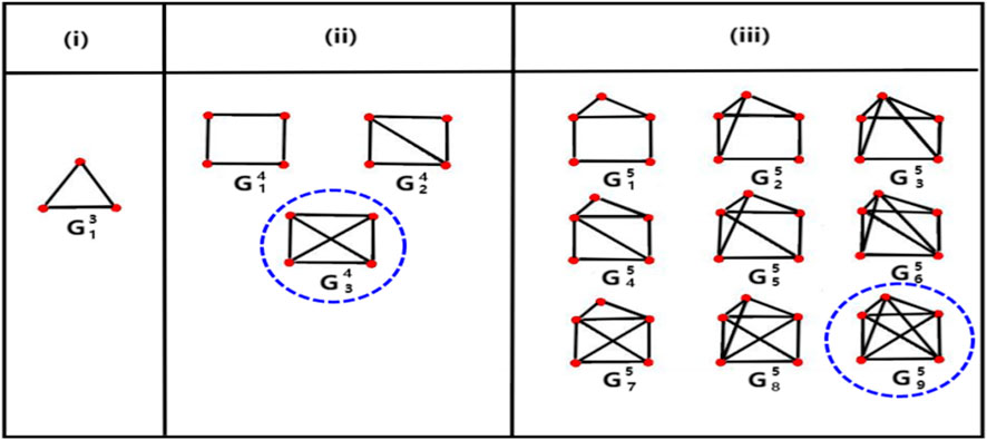
FIGURE 1. From (i–iii), they are third-order, fourth-order and five-order, respectively. Where $G_i^k$ represents the ith k-order structure. It can be seen that the variety of higher order structures grows exponentially as the order increases. In (i), there exists only a unique higher-order structure, i.e., $G_1^3$. In (ii,iii), all of them are partially connected except for $G_3^4$ and $G_9^5$ which are fully connected.

2.3.2 High-order node degree

The traditional node clustering coefficient measures how many triangles with the node as the vertex in the first-order neighborhood, i.e., how sparsely the neighboring nodes are connected to each other in the first-order neighborhood. The formula is:

$C_i=\frac{2L_i}{k_i\left(k_i-1\right)}(4)$

Where, $L_i$ represents the actual number of links in the first-order neighborhood of node i, and $k_i\left(k_i-1\right)/2$ represents the maximum number of all possible links formed. The traditional node clustering coefficient only takes into account the connections among neighbors in first-order neighborhoods, as shown in Figure 2, $k_a^{∆}=6$, where $∆$ is the number of triangles with a as the vertex. This local metric uses only information from the first-order neighbors to determine the importance of the nodes. Inspired by this, we enrich the variety of higher-order structures, extending the range to second-order neighborhoods to determine the importance of nodes. High-order node degree is defined as the sum of the number of triangles, diagonal quadrilateral and fully connected quadrilateral in the first-order neighborhood of a node and the number of diagonal quadrilateral and loops in the second-order neighborhood. Expressed as $k^{\mathrm{\Phi }}$. As shown in Figure 2, $k_a^{\mathrm{\Phi }}=$ 10, $\mathrm{\Phi }$ is the number of higher-order structures of the node a involved in the first and second-order neighborhoods. This is actually a semi-local measure, and the analysis range is increased to include higher order structures in second-order neighborhoods, extending from triangles to higher-order quadrilaterals. To determine the importance of a node, in addition to using node information from first-order neighborhoods, node information from second-order neighborhoods is used to improve accuracy. At the same time, this does not significantly increase the time complexity of the computation.

FIGURE 2

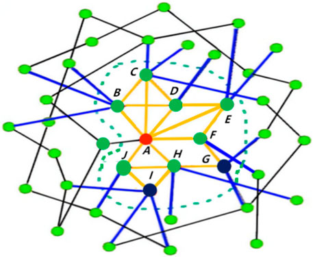
FIGURE 2. A toy networks. In the first-order neighborhood of node A (red), the nodes located on the same higher-order structure with node A are B、C、D、E、F、H、J (green). The second-order neighbor nodes located on the same higher-order structure as node A are G and I (black). The triangle in the first-order neighborhood of node A are ABC、ABD、ACD、ADE、AEF、AHJ, the diagonal quadrilateral is ADEF, a fully connected quadrilateral is ABCD. The diagonal quadrilateral in the second-order neighborhood of node A is AHIJ, the empty quadrilateral (loop) is AFGH. In addition, the yellow link represents the internal link of the small community formed by the four types of high-order structures in the first and second-order neighborhood of node A, the blue links represent the small community’s links to external contacts.

2.3.3 Effect of the higher-order structure on the propagation dynamics

Several studies have shown that the presence of higher-order interactions may severely affect the dynamics of network systems, from diffusion [26, 27] and synchronization [28, 29] to social [30–33] and evolutionary processes [34], possibly leading to the emergence of abrupt (explosive) transitions between states. Under different mechanisms of simple and complex contagion, the presence of higher-order structures can make the propagation process on the network significantly different [35–38]. Diffusion is often described as either “simple contagion” or “complex contagion”, where simple contagion is a process in which a node is easily infected through a single contact with an infected neighbor. Complex infection is a collaborative merged infection process in which nodes are usually exposed to multiple infected neighbors multiple times before changing state. Under a simple transmission mechanism, infected nodes transmit the virus through their links at a fixed infection rate per unit time. Predisposing nodes change states and become infected, whose rate is related linearly to the number of infected neighbors. In the complex contagion definition of disease interactions, a susceptible node is co-infected by more than one neighboring infected node. In fact, there exists a threshold of co-infection beyond which the threshold is exceeded. As the infection rate increases, the clustered network structure will enhance the propagation of the co-combination infection. This is the reinforcement mechanism from the higher order structure. As shown in Figure 3, the different infection pathways of susceptible node i are shown. Under the simple infection mechanism, node i contacts with one (A, C) or more (B, D) infected nodes through the links and is infected at each time step at the rate $\mathrm{\lambda }$ through these links. In E, nodes i, j are infected by the triangle at the infection rate ${\lambda }_1^{*}$. In G, node i is infected by the fully connected quadrilateral at the infection rate ${\lambda }_3^{*}$. We would like to highlight F, which has been ignored in previous higher-order contagion models. It is believed that node e is not directly connected to i, so the two cases E and F are confused. In fact, these two cases should be discussed separately. Although node e is not directly connected to i, e exerts its influence directly on the triangle to act indirectly on i. This is for the real-life scenario with strongly superimposed viruses, so the contagion is stronger than E. The infection rates for all cases are roughly ordered, i.e., ${\lambda }_3^{*}$ > ${\lambda }_2^{*}$ > ${\lambda }_1^{*}$ > $\lambda$.

FIGURE 3

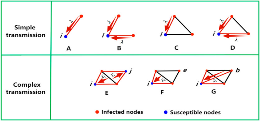
FIGURE 3. There are simple contagion and complex contagion. (A–D) for simple contagion. In the case of complex contagion we have (E–G). Because of the higher-order interaction, the rate of infection varies with different modes of contagion. $\lambda$ represents the transmission rate under the simple transmission mechanism, ${\lambda }_1^{*}$ represents the transmission rate under the complex transmission mechanism in the form of links, ${\lambda }_2^{*}$ represents the transmission rate under the complex transmission mechanism in the form of triangles, ${\lambda }_3^{*}$ represents the transmission rate under the complex transmission mechanism in the form of triangles and links.

3 The proposed method

The node importance metric proposed in this paper is a generalization of the traditional clustering coefficients of nodes. The scope is extended from the first-order neighborhood of nodes to the second-order neighborhood, the types of higher-order structures are extended from a single triangle to loops and quadrilaterals. In terms of the topology of the network, the influence of the loop structure on the propagation is also taken into account. In terms of propagation mechanism, the influence of fully connected quadrilateral and diagonal quadrilateral on the propagation of viruses with mutual superposition is considered. The equation of the metric is expressed as follows:

$CK\left(i\right)=\frac{k_i^{\mathit{\Phi }}}{N_{\alpha }+N_{\beta }}\times \frac{L^{ext}}{L^{\mathit{int}}+L^{ext}}(5)$

Where $N_{\alpha }=k_i(k_i-1$) $∕$ 2 + $2k_i!/3!\left(k_i-3\right)!$ represents the maximum number of triangles, diagonal quadrangles and fully connected quadrangles in the first-order neighborhood of node i. $N_{\beta }=k_i\left(k_i-1\right)\times k_i^2$ represents the sum of the maximum number of diagonal quadrilateral and loops in the second-order neighborhood of node i. $k_i,k_i^2$ representing the number of nodes in the first and second-order neighborhoods, respectively. $L^{\mathit{int}}\mathrm{a}\mathrm{n}\mathrm{d}{L}^{ext}$ are the inner links (Links between nodes located on higher-order structures within the first and second-order neighborhoods of a node, such as the yellow edges in Figure 2) and the outer links (Links with only one node located on higher-order structures within first and second-order neighborhoods, such as the blue edges in Figure 2), respectively. In fact we can consider the region containing the higher-order structure within the second-order neighborhood of a node as a small community. $\frac{L^{ext}}{L^{\mathit{int}}+L^{ext}}$ is used to portray the difference in density inside and outside the community. In a complex mechanism of propagation, the community is seen locally as a “accelerator” of propagation, a high density of external links will ensure that the spread is global. $0\le CK\left(i\right)\le 1$. Note that this formula is only applicable to the case of $k_i\ge 3$. At the same time, the measurement we propose is only applicable to undirected and unweighted networks.

According to the proposed node importance measure, we take node A in Figure 2 as an example to calculate its CK value. $k_A^{\mathit{\Phi }}$ = 10, $N_{\alpha }=8(8-1$) $∕$ 2 + $2\times 8!/3!\left(8-3\right)!=$ 140 and $N_{\beta }=8\left(8-1\right)\times 17=$ 952. $L^{ext}=17,L^{\mathit{int}}=18.$ So the CK of node A in Figure 2 is $CK\left(A\right)=\left(10\right./1092)\times \left(17/35\right)\approx 0.004$. Next, let’s consider the computational complexity of the proposed importance measure. For a network with n nodes, the average degree of nodes is $〈k〉$, the computational complexity of calculating the number of first-order neighbors of each node $\mathrm{i}\mathrm{s}\mathrm{{\rm O}}\left(〈k〉\right)$, the computational complexity of calculating the number of second-order neighbors of each node is $\mathrm{{\rm O}}\left({〈k〉}^2\right)$, then the total computational complexity is $\mathrm{{\rm O}}\left(n〈k〉\left(〈k〉+1\right)\right)$. Therefore, the near linear computational complexity makes the proposed metric scalable to large-scale networks. For $k_i^{\mathit{\Phi }}$, it is not easy to find the high-order vertex degree of node i in large dense networks. In this paper, we also propose a method to quickly find all the above higher-order structures using only the adjacency matrix of the nodes within the second-order neighborhood containing node i. See Supplementary Material.

4 Experimental setup

4.1 Data set

In order to test the effectiveness of the proposed method, we apply it to real-world networks and artificial networks. Real world networks include (i) electricity: the network of power grids; (ii) network science: the coauthor network in network science consists of 1,589 nodes. We chose the largest dense community of 400 nodes in this network. (iii) Email: the email network of the University Rovirai Virgili. (iv) Yeast: the protein-protein interaction network. The two artificial networks are Watts-Strogatz (WS) small world network [39] and Barabasi-Alber (BA) scale-free network [40]. First, a small world network (WS) is constructed, in which nodes $n$ = 1,000, links $m$ = 1,475, nodes are connected with a probability of $p$ = 0.01. The average degree of the network is <k>≈3. The scale-free network (BA) takes N = 1,000, $m_0$ = 5, $m$ = 4 (for the initial network with $m_0$ nodes, each time a new node is introduced to connect with $m$ existing nodes, $m$ ≤ $m_0$), generates a scale-free network with N = 1,000 nodes and $mt$ = 3,980 links ($t$ steps are required to generate the required scale-free network). Table 1 shows the statistical characteristics of six networks. In this paper, all these real-world networks and analog network are regarded as undirected and unweighted.

TABLE 1

TABLE 1. Some statistical properties of six networks. Its topological features include: number nodes ($\left|V\right|$), number of edges $\left(|E\right|$), average degree $\left(\langle k\right.〉$), maximum degree ($k_{\mathit{max}}$), average clustering coefficient ($〈C〉$), propagation threshold (${\lambda }_{th}^{*}$ = $〈k〉/〈k^2〉$).

4.2 Dynamic transmission model

To compare the accuracy of the proposed metric in identifying node propagation capabilities, the susceptible infection (SI) model is used to simulate propagation and evolution in real networks. The SI model contains only two types of nodes, susceptible (S) and infected (I). Once a node is infected, it will never be able to recover. Assume that the total network scale of disease transmission is N, S(t) represents the number of susceptible nodes at time t, I(t) represents the number of infected nodes at time t (S(t) + I(t) = N). At t = 0, all nodes are susceptible, that is S (0) = N and I(t) = 0. At t = 1, we selected a node in the network as the initial source of infection. It is assumed that each node has $〈k〉$ contactable neighbor nodes in unit time $∆t$ (here approximated by the average degree of the network) and $〈k_1〉$ of these $〈k〉$ neighbor nodes are susceptible, the initial transmission rate of the disease from infected nodes to susceptible nodes is $\lambda$. At each time step $∆t$, infected nodes can simultaneously spread the virus to more than one susceptible node. According to the assumption of uniform mixing (each node will touch the infected node with equal probability), the probability of an infected node encountering a susceptible node is $\frac{S\left(t\right)}{N}$, so the infected node will contact $\frac{〈k_1〉}{〈k〉}\bullet \frac{S\left(t\right)}{N}$ susceptible nodes per unit time. Since there are I(t) total of infected nodes at time t to spread the disease with the transmission rate $\lambda$, the average number of newly infected nodes dI(t) within the differential time dt is: $dI\left(t\right)$ = $\lambda \bullet$ I(t) $\bullet \frac{〈k_1〉}{〈k〉}\bullet \frac{S\left(t\right)}{N}$ dt. In other words, the rate of change of I(t) is: $\frac{dI\left(t\right)}{dt}$ = $\lambda \frac{〈k_1〉}{〈k〉}\bullet \frac{I\left(t\right)\bullet S\left(t\right)}{N}$.

In this paper, we use SI model under complex propagation mechanism. This is different from the SI model in the simple transmission mechanism because we consider the strengthening mechanism of the higher-order structure in the transmission process and define that the diseases can be superimposed and co-infected. In our model, as soon as the initial infected node infects the node on the same link as it, the complex propagation mechanism will be triggered and the complex propagation process will begin in the form of a link. At the same time, the propagation rate does not remain constant, but increases gradually with the participation of more and more higher-order structures. In this case, the transmission rate is ${\lambda }^{*}$ = c $\bullet \lambda$. Where c is a perturbation parameter, it increases with the increase of the number of participating higher-order structures in the propagation process, that is the more involved higher-order structures, the faster c increases, and vice versa. As time increases more and more higher-order structures are involved in the propagation process, the virus becomes more contagious and spreads faster and more widely. Figure 4 shows the basic propagation process under the complex propagation model, where red nodes are infected nodes and blue nodes are susceptible nodes. At the initial time $t_0$, a node is selected as the initial source of infection. With the progress of transmission, ${∆t}_1>{∆t}_2$ and ${\lambda }_1^{*}<{\lambda }_2^{*}$ can be obtained by involving more and more higher-order structures. In addition, the outbreak of the propagation process is related to the propagation threshold [8]. If the transmission rate is much smaller than the threshold, the transmission process will be limited to a smaller area and will end prematurely. Conversely, if the transmission rate is much greater than the threshold, the transmission process will spread instantaneously over a large part of the network. Therefore, it is reasonable to choose a transmission rate near the neighborhood of the propagation threshold to evaluate the validity of a centrality metric. That is, a transmission rate that is too small will result in a diffusion process of limited size and affect the accuracy of the observation. In contrast, too large a value of the transmission rate will lead to a large-scale diffusion of the network, the propagation ability of individual nodes cannot be identified. Notice here that, unlike simple propagation, the propagation threshold is based on a complex propagation mechanism.

FIGURE 4

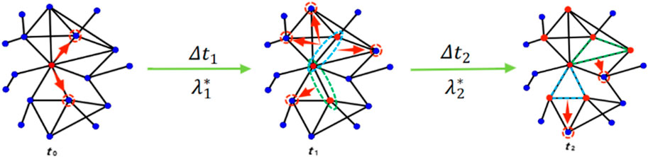
FIGURE 4. An evolutionary diagram of a complex propagation process. The red nodes are infected nodes and the blue nodes are susceptible nodes.

5 Evaluation methods

From the perspective of propagation dynamics, the greater the influence of a node, the stronger the diffusion ability of the node. That is, the number of nodes in the network that are ultimately infected is more. We use the number of final infected nodes $F_i\left(t_c\right)$ after $t_c$ time step to reflect the propagation ability of nodes in the network. The formula is as follows:

$F_i\left(t_c\right)=\frac{1}{M}{\displaystyle \sum _{m=1}^M}{f}_i\left(m\right)(6)$

Where, M is the total number of experimental repetitions, $f_i\left(m\right)=n_i/N$ is the proportion of the final infected nodes in the steady state of the network. Set the propagation threshold of propagation rate ${\lambda }^{*}>{\lambda }_{th}^{*}$, where $〈k〉$ and $〈k^2〉$ are the average degree and the variance respectively. We assume that at the beginning, all nodes in the network are susceptible except the initial infection source.

Kendall’s tau correlation coefficient is selected to determine the consistency between the ranking list obtained by the specific measurement method and ranking list obtained by SI model based on standard Monte Carlo simulation. Give two ranking lists X and Y, $\left(x_i,y_i\right)$ and $\left(x_j,y_j\right)$ are the two node pairs in these lists. The Kendall’s tau correlation coefficient is defined as:

${\tau }_{\left(X,Y\right)}=\frac{2\left(n_1-n_2\right)}{N\left(N-1\right)}(7)$

In this paper, X represents the ranking result of nodes obtained from a centrality measure, and Y represents the ranking result of the number of infected nodes obtained from the SI model based on standard Monte Carlo simulation. If $x_i>x_j$, $y_i>y_j$ or $x_i<x_j,y_i<y_j$. That is to say $x_i,x_j$ the order in X is the same as $y_i$, $y_j$ in y. Otherwise, it is called inconsistent. $n_1$ and $n_2$ represents the number of consistent and inconsistent pairs, N is the length of the sorting list X. Obviously, $\tau$ between −1 and 1. Here, $\tau =-1$ it means that the order of these two lists is completely opposite. At that time, $\tau =1$, the order of the two lists was the same.

In order to distinguish the propagation ability of all nodes, each node should assign a unique indicator through centrality measurement. The proportion of repeating elements in a sequence is called the monotonicity of the sequence. In order to quantify the monotonicity of different sorting methods, we use [8] and define it as:

$M\left(R\right)=\left[1-\frac{{\displaystyle \sum }_{r\in R}{N}_r\left(N_r-1\right)}{N\left(N-1\right)}\right](8)$

Where $N$ is the length of the ranking list R, $N_r$ indicating the number of nodes with the same sorting value R. The range of M values is 0–1. The best value of M is 1, which means that each node in the network has a unique and identifiable sorting value. On the contrary, the worst value of M is 0, which means that all nodes in the network have the same ranking.

Pearson coefficient (R) is used to explain the correlation between different sorting methods. The formula of R is as follows [22]:

$R=\frac{{\displaystyle \sum _{i=1}^n}\left(X_i-\overline{X}\right)\left(Y_i-\overline{Y}\right)}{\sqrt{{\displaystyle \sum _{i=1}^n}{\left(X_i-\overline{X}\right)}^2}\times \sqrt{{\displaystyle \sum _{i=1}^n}{\left(Y_i-\overline{Y}\right)}^2}}(9)$

Where, $X_i,Y_i$ represents the set of propagation capacity of each node in the network under any two different sorting methods, where $X_i=\left(x_1,x_2,...,x_n\right),Y_i=\left(y_1,y_2,...,y_n\right).\left(x_i,y_i\right)$ represents the combination of propagation capabilities of the same node under two different sorting methods. For an N node network, there will be such a combination are the average of $N\left(N-1\right)∕$ 2. The value of R is between [−1,1]. R = 1, then the two sorting methods show positive linear correlation; R = 0, then the two sorting methods are irrelevant; R = −1, then the two sorting methods are negative linear correlation. When R is in [0,1], the two sorting methods are positively correlated, and the closer to 1, the stronger the positive correlation; When R is at [−1,0], the two sorting methods are negatively correlated, and the closer to −1, the stronger the negative correlation.

6 Experimental results and analysis

In the experiments, the proposed node importance metric was compared with three other metrics, including CR, FI, and SHF. We use different methods to analyze the performance of the proposed centrality metric in terms of propagation ability, correlation and monotonicity.

6.1 Analysis of transmission capacity

At time step t = 1, the nodes with the largest values of SHF, FI, CR, and CK are selected as the initial infection sources. Set the initial transmission rate of the disease to be slightly greater than the propagation threshold of the network. The final proportion of infected nodes in the six networks was observed after 100 time steps. The experimental results are shown in Figure 5, it can be seen from Figures 5A-E that the proposed metric CK results in the largest proportion of final infected nodes after 100 time steps. This is followed by FI, SHF, and CR. In fact, under the complex contagion mechanism, nodes with larger FI metric values have dense second-order neighbors and their second-order neighbors are part of the dense part of the network, the disease triggers the complex contagion mechanism once it spreads to the second-order neighbors of the node, which facilitates the global spread of the disease. However, the clustering coefficients of the nodes are small, which makes it harder for the initial spread of the disease to trigger complex contagion on a large scale, so the FI is ultimately secondary to the CK. For SHF, this metric only considers the degree of node and the number of common neighbors in the first-order neighborhood. Therefore, the initial spread of the disease is carried out under complex transmission with triangles and subsequently spreads to second-order neighborhoods. This inhibits the spread of the disease to some extent due to the lack of information related to the second-order neighborhood, so the SHF is ultimately subordinate to the FI. It is difficult to trigger complex propagation with an infection source on a loop (except for triangles), this is mainly because all nodes on the loop except the nodes at both ends of the link cannot achieve direct interaction, i.e., the loop lacks higher-order structures that trigger complex contagion, so it can be seen that the CR metric has the lowest number of final infected nodes. In Figure 5F, it can be seen that the only difference is that the propagation rate of FI is slightly greater than CK after t = 35. This is mainly because BA is a network of many small communities connected by the large-degree nodes and FI happens to identify the large degree nodes in the BA network. The tight clustering maximizes the complex propagation mechanism when the virus propagates to the second-order neighborhoods of the nodes identified by the FI. In addition, we looked at disease transmission rates over 100 time steps. Here we set the initial transmission of the disease is slightly greater than that of each network propagation threshold value, which in turn were 0.26, 0.14, 0.06, 0.065, 0.16, and 0.10. The results are shown in Figure 6. It can be seen that when the node identified by metric index CK is taken as the initial transmission source, the transmission rate of the disease in the 6 networks is always the largest in 100 time steps. This also shows from the side that there are the most high-order structures involved in the whole propagation process and further explains the accuracy of CK in identifying the most important nodes under the complex propagation mechanism. In Eqs 1, 4–6, the effect of measurement index FI is better than that of SHF. In Eq. 2, the effect of FI and SHF is roughly equivalent. In Eq. 3, SHF is superior to FI. However, the effect of CR is always the worst in the six networks. Secondly, the measurement index FI in Eq. 6 also has a good effect. To sum up, under the complex transmission mechanism based on SI model, when the node identified by the metric index CK is the initial infection source, the number of nodes infected and disease transmission rates in the network will be the largest after 100 time steps.

FIGURE 5

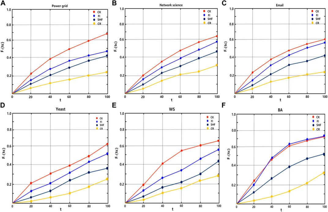
FIGURE 5. The number of final infected nodes caused by four different centrality measures on six networks in (A-F). The horizontal axis corresponds to the infection time and the vertical axis represents the diffusion capacity $F_i\left(t_c\right)$. The results are averaged by 100 independent experiments on the complex SI model.

FIGURE 6

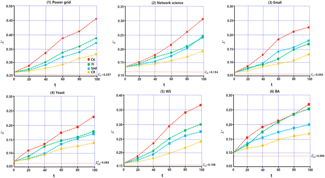
FIGURE 6. Network propagation rate ${\lambda }^{*}$ as a function of time t in (1), (2), (3), (4), (5) and (6). Each network is the average result of 200 separate simulations on the complex SI model.

6.2 Kendall’s tau correlation coefficient

In order to test the accuracy of the proposed centrality measure, it is compared with three different centrality measures on six networks under the complex SI model. The closer to 1 is $\tau$, the better the performance of the sorting method. The selection value ${\mathrm{\lambda }}^{*}$ changes near the propagation threshold. The value ${\lambda }_{th}^{*}$ is related to the topological characteristics of a given network, so the abscissa of different networks in Figure 6 is different. Figure 7 describes the Kendall’s tau correlation coefficient of four central indicators varying with the probability of infection. In Figures 7G-K, CK was superior to the other three centrality indicators over the entire range of infection probabilities. In Figure 7G, the $\tau$ values of CK and FI were roughly equivalent around the prevalence threshold. This is mainly because ${\mathrm{\lambda }}^{*}$ as a relatively small value, the influence of the node is limited to a small range resulting in the virus not spreading. It can be seen that CK gradually outperforms FI as ${\mathrm{\lambda }}^{*}$ increases. In Figure 7H, K, the four centrality measures differed most from each other. This is mainly because Network science and WS networks are characterized by large clustering coefficients and small average path lengths, which create the most powerful conditions for triggering complex propagation mechanisms. The complex contagion is triggered at the initial propagation, which makes CK the most accurate in identifying the important nodes. At the same time, SHF is superior to FI when ${\lambda }^{*}$ is in [0.124, 0.135] and [0.157, 0.195], which is also due to the larger clustering coefficients. Because SHF takes into account the number of common neighbors in the first-order neighborhood of a node while FI does not, this leads to a decrease in the accuracy of FI in identifying influential nodes for period of time when ${\lambda }^{*}$ exceeds ${\lambda }_{th}^{*}$. In Figure 7L, CK is better than FI before ${\lambda }^{*}$ = 0.093. This is because BA is composed of “hub” nodes connecting many dense small communities, which can trigger less complex propagation during the initial propagation of the virus because there are fewer higher-order structures in the first-order neighborhoods of the nodes identified by FI. At after ${\lambda }^{*}$ = 0.093, FI is gradually better than CK. Because as the virus continues to spread to second-order neighborhoods, the dense cluster of the second-order neighborhoods of FI-identified nodes plays a huge role in triggering complex propagation, which greatly improves the accuracy of the FI metric. Furthermore, we can see that the $\tau$-value of CR is the lowest among all networks, which means that CR cannot identify important nodes under the complex propagation mechanism. It can be seen that under the complex propagation mechanism based on SI model, the $\tau$ value of the metric index CK is always the highest, which also means that most nodes identified by CK are the nodes with the strongest propagation ability in the network.

FIGURE 7

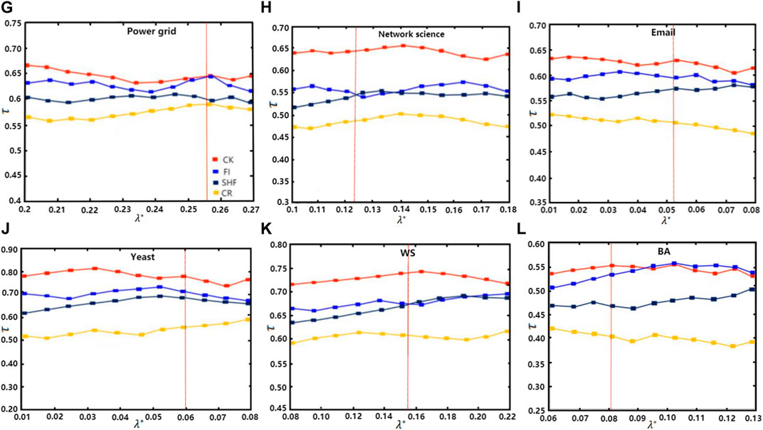
FIGURE 7. The Kendall’s tau correlation coefficient ($\tau$) between the ranking results obtained from the four different metrics and the $F_i\left(t_c\right)$ ranking list obtained from the SI model with different infection probabilities ${\lambda }^{*}$ in (G-L), ${\lambda }^{*}$ Changes near the neighborhood of ${\lambda }_{th}^{*}$. The results obtained by averaging 100 independent simulations of the complex SI model, where the vertical dotted line represents the propagation threshold ${\lambda }_{th}$.

6.3 Monotonicity

A good centrality measure should be able to distinguish between nodes with different propagation capabilities. Table 2 shows the monotonicity of the four centrality measures in six different networks. The closer M is to 1 the better the performance of the centrality measure is. It can be seen that among the four centrality measures, the monotonicity value of CK (black bold) is always close to 1 in all networks. In summary, CK can better distinguish nodes with different propagation capabilities. We conclude that under the complex propagation mechanism based on SI model, the metric index CK can well distinguish nodes with different propagation capabilities in the network.

TABLE 2

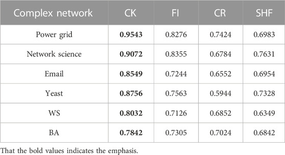
TABLE 2. Monotonicity of four centrality measures in six networks.

6.4 Correlation analysis

Figure 8 shows the correlation matrix between CK and the other three centrality metrics. Each of these elements represents the average of the correlation coefficient r between the two metrics over the six networks, the results are accurate to two decimal places. It can be seen that CK, FI has the strongest correlation, followed by CK SHF、CK CR. This is because FI considers triangles in the first-order neighborhood of a node, diagonal quadrilateral and loops in the second-order neighborhood. SHF considers only triangles in the first-order neighborhood of a node. CR only considers the loops in the second-order neighborhood of the node. The proposed metric CK based on the higher-order vertex degree of the node not only considers the loop in the second-order neighborhood but also the diagonal quadrilateral, the fully connected quadrilateral in the first-order neighborhood and the diagonal quadrilateral, which is an extension of the other three metrics considering a more diverse higher-order structure. The same result is obtained from Figure 9. Each point denotes one node in the network, the color of the node indicates the nodal spreading ability simulated by the complex SI model, denoted by $F_i\left(t_c\right)$ ($t_c$ = 100). Note that the more propagating a node is, the closer its color is to red. In (m) (q) (v), we can clearly see that CK and FI have the strongest correlation, followed by CK, SHF, and CK, CR. The correlation between CK and CR is weak, because many nodes are assigned the same value. Furthermore, the larger the value of CK, the redder the color of the node, which is in accordance with the actual spreading ability $F_i\left(t_c\right)$ of nodes. It can be seen that when identifying the nodes with the strongest propagation ability in the network under the complex propagation mechanism, if the metric index CK is not available, FI may be an optimal alternative.

FIGURE 8

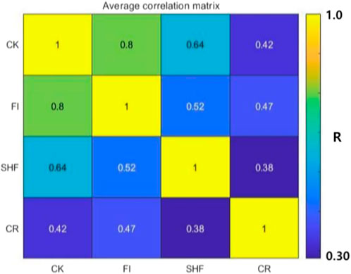
FIGURE 8. The average correlation matrix for the four indices of node importance over six networks. Each element is the averaged value of the correlation R between the two indices corresponding to its position over the six networks, and the value is visualized by the color. The correlation increases gradually from blue to yellow.

FIGURE 9

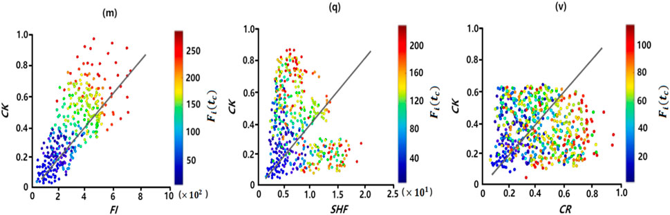
FIGURE 9. Average correlation between the proposed CK centrality and the other three measures of centrality in the six networks in (m), (q) and (v). Each point represents a node, and its color denotes the $F_i\left(t_c\right)$ ($t_c$ = 100) value of the node. The data are obtained from the complex SI model by averaging the results of 100 independent simulations on six networks when ${\lambda }^{*}>{\lambda }_{th}$.

7 Conclusion

In this paper, a new node importance metric is proposed for identifying nodes with the strongest propagation capacity under complex contagion mechanisms. The metric innovatively considers diagonal quadrilateral, loop (empty quadrilateral) and fully connected quadrilateral in the first and second-order neighborhood of a node. The impact of these structures on the complex propagation dynamics on the network is considered. Meanwhile, the high-order node degree are defined and a complex propagation model which has been neglected in the past is introduced. The superiority of the proposed metric is obtained by analyzing the simulation results on real and synthetic networks. In addition, only some of the higher-order forms in the first and second-order neighborhoods of the nodes are considered in this paper, in fact their higher-order structures are much richer than we can imagine. Moreover, as the analysis range (the neighborhood of nodes) extends outward, its computational complexity is exponentially increasing, and we will face more difficult problems. This work will be explored in the next step. Our future work will mainly focus on finding the optimal combination of higher-order structures in the node’s neighborhood that can most efficiently facilitate the information dissemination. At the same time, we will also propose some targeted protection strategies for the higher-order organization of the network.

Data availability statement

The raw data supporting the conclusion of this article will be made available by the authors, without undue reservation.

Author contributions

JS proposed the advice and conducted the numerical experiments. GW checked the paper in the later stage. All authors contributed to the article and approved the submitted version.

Acknowledgments

We would like to thank all the anonymous reviewers for their helpful suggestions to improve the quality of our manuscript.

Conflict of interest

The authors declare that the research was conducted in the absence of any commercial or financial relationships that could be construed as a potential conflict of interest.

Publisher’s note

All claims expressed in this article are solely those of the authors and do not necessarily represent those of their affiliated organizations, or those of the publisher, the editors and the reviewers. Any product that may be evaluated in this article, or claim that may be made by its manufacturer, is not guaranteed or endorsed by the publisher.

Supplementary material

The Supplementary Material for this article can be found online at: https://www.frontiersin.org/articles/10.3389/fphy.2023.1046077/full#supplementary-material

References

1. Domenico MD, Solé-Ribalta A, Omodei E. Ranking in interconnected multilayer networks reveals versatile nodes. Nat Commun (2017) 6:6868. doi:10.1038/ncomms7868

CrossRef Full Text | Google Scholar

2. Li M, Liu RR, Lü L, Hu MB, Xu S, Zhang YC. Percolation on complex networks: Theory and application. Phys Rep (2021) 907:1–68. doi:10.1016/j.physrep.2020.12.003

CrossRef Full Text | Google Scholar

3. Freeman LC. Centrality in social networks conceptual clarification. Social Networks (1978) 79:215–39. doi:10.1016/0378-8733(78)90021-7

CrossRef Full Text | Google Scholar

4. Latora V, Marchiori M. A measure of centrality based on the network efficiency. open-access J Phys (2004) 402:345–51. doi:10.1103/85.066127

CrossRef Full Text | Google Scholar

5. Arruda GD, Petri G, Rodrigues FA. Impact of the distribution of recovery rates on disease spreading in complex networks. Phys Rev Res (2018) 5:1012. doi:10.1103/PhysRevResearch.2.013046

CrossRef Full Text | Google Scholar

6. Kitsak M, Gallos LK, Havlin S, Liljeros F, Muchnik L, Stanley HE, et al. Identification of influential spreaders in complex networks. Nat Phys (2010) 6:888–93. doi:10.1038/nphys1746

CrossRef Full Text | Google Scholar

7. Chen DB, Gao H, Linyuan L, Zhou T. Identifying influential nodes in large-scale directed networks: The role of clustering. PLoS ONE (2013) 8:e77455. doi:10.1371/journal.pone.0077455

PubMed Abstract | CrossRef Full Text | Google Scholar

8. Xu GQ, Meng L, Tu DQ, Yang PL. Lch: A local clustering H-index centrality measure for identifying and ranking influential nodes in complex networks*. Chin Phys B (2021) 30:088901. doi:10.1088/1674-1056/abea86

CrossRef Full Text | Google Scholar

9. Salavati C, Abdollahpouri A, Manbari Z. Ranking nodes in complex networks based on local structure and improving closeness centrality. Neurocomputing (2019) 336:36–45. doi:10.1016/j.neucom.2018.04.086

CrossRef Full Text | Google Scholar

10. Ruan Y, Tang J, Wang H, Guo J, Qin W. Method for measuring node importance in complex networks based on local characteristics. Int J Mod Phys B (2021) 18:174–86. doi:10.1142/S0217979221502313

CrossRef Full Text | Google Scholar

11. Shao Z, Liu S, Zhao Y, Liu Y. Correction to: Identifying influential nodes in complex networks based on Neighbours and edges. Peer-to-Peer Networking Appl (2018) 12:1538–7. doi:10.1007/s12083-018-0686-5

CrossRef Full Text | Google Scholar

12. Hu P, Mei T. Ranking influential nodes in complex networks with structural holes. Physica A (2018) 490:624–31. doi:10.1016/j.physa.2017.08.049

CrossRef Full Text | Google Scholar

13. Qiang L, Zhu Y, Yan J. Leveraging local h-index to identify and rank influential spreaders in networks. Physica A (2017) 512:379–91. doi:10.1016/j.physa.2018.08.053

CrossRef Full Text | Google Scholar

14. Hajarathaiah K, Enduri MK, Anamalamudi S. Efficient algorithm for finding the influential nodes using local relative change of average shortest path. Physica A (2022) 591:126708. doi:10.1016/j.physa.2021.126708

CrossRef Full Text | Google Scholar

15. Guo C, Yang L, Chen X, Chen D, Gao H, Ma J. Influential nodes identification in complex networks via information entropy. Entropy (2020) 22(2):242. doi:10.3390/e22020242

PubMed Abstract | CrossRef Full Text | Google Scholar

16. Wen T, Deng Y. Identification of influencers in complex networks by local information dimensionality. Inf Sci (2020) 512:549–62. doi:10.1016/j.ins.2019.10.003

CrossRef Full Text | Google Scholar

17. Fan C, Zeng L, Sun Y, Liu YY. Finding key players in complex networks through deep reinforcement learning. Nat Machine Intelligence (2020) 2:317–24. doi:10.1038/s42256-020-0177-2

CrossRef Full Text | Google Scholar

18. Fan T, Lü L, Shi D. Towards the cycle structures in complex network: A new perspective. Phys Soc (2019) 3:1–22. doi:10.48550/arXiv.1903.01397

CrossRef Full Text | Google Scholar

19. Fan T, Lü L, Shi D, Zhou T. Characterizing cycle structure in complex networks. Nat Commun (2020) 4:272. doi:10.1038/s42005-021-00781-3

CrossRef Full Text | Google Scholar

20. Zhang WJ, Li W, Deng WB. The characteristics of cycle-nodes-ratio and its application to network classification. Commun Nonlinear Sci Numer Simulation (2021) 1007:105804. doi:10.1016/j.cnsns.2021.105804

CrossRef Full Text | Google Scholar

21. Chen DB, Sun HL, Tang Q, Tian SZ, Xie M. Identifying influential spreaders in complex networks by propagation probability dynamics. Chaos (2019) 29:033120. doi:10.1063/1.5055069

PubMed Abstract | CrossRef Full Text | Google Scholar

22. Kamal B, Asgarali B, Samadi N. A new centrality measure based on the negative and positive effects of clustering coefficient for identifying influential spreaders in complex networks. Chaos Solitons & Fractals (2018) 110:41–54. doi:10.1016/j.chaos.2018.03.014

CrossRef Full Text | Google Scholar

23. Lei W, Xu G, Yang P, Tu D. A novel potential edge weight method for identifying influential nodes in complex networks based on neighborhood and position. J Comput Sci (2022) 60:101591. doi:10.1016/j.jocs.2022.101591

CrossRef Full Text | Google Scholar

24. Gupta M, Mishra R. Spreading the information in complex networks: Identifying a set of top- N influential nodes using network structure. Decis Support Syst (2021) 149:113608. doi:10.1016/j.dss.2021.113608

CrossRef Full Text | Google Scholar

25. Burt RS. Structural holes: The social structure of competition[J]. Econ J (1994) 40(2). doi:10.2307/2234645

CrossRef Full Text | Google Scholar

26. Battiston F, Amico E, Barrat A, Bianconi G, Ferraz de Arruda G, Franceschiello B, et al. The physics of higher-order interactions in complex systems. Nat Phys (2021) 17:1093–8. doi:10.1038/s41567-021-01371-4

CrossRef Full Text | Google Scholar

27. Schaub MT, Benson AR, Horn P, Lippner G, Jadbabaie A. Random walks on simplicial complexes and the normalized hodge 1-laplacian. SIAM Rev (2018) 62:353–91. doi:10.1137/18M1201019

CrossRef Full Text | Google Scholar

28. Mulas R, Kuehn C, Bhle T, Jost J. Random walks and Laplacians on hypergraphs: When do they match? Discrete Appl Math (2021) 317:26–41. doi:10.1016/j.dam.2022.04.009

CrossRef Full Text | Google Scholar

29. Millán AP, Torres JJ, Bianconi G. Synchronization in network geometries with finite spectral dimension. Phys Rev E (2019) 99:022307. doi:10.1103/PhysRevE.99.022307

PubMed Abstract | CrossRef Full Text | Google Scholar

30. Skardal PS, Arenas A. Abrupt desynchronization and extensive multistability in globally coupled oscillator simplices. Phys Rev Lett (2019) 122(24):248301.1–248301.6. doi:10.48550/arXiv.1903.12131

CrossRef Full Text | Google Scholar

31. Iacopini I, Petri G, Barrat A, Latora V. Simplicial models of social contagion. Nat Commun (2018) 10:2485. doi:10.1038/s41467-019-10431-6

CrossRef Full Text | Google Scholar

32. Guilherme F, Petri G, Rodriguez PM. Multistability, intermittency and hybrid transitions in social contagion models on hypergraphs (2021). Available at: https://arxiv.org/abs/2112.04273 (Accessed December 8, 2021).

Google Scholar

33. Neuhuser L, Mellor A, Lambiotte R. Multibody interactions and nonlinear consensus dynamics on networked systems. Phys Rev E (2022) 101:032310. doi:10.1103/PhysRevE.101.032310

CrossRef Full Text | Google Scholar

34. Alvarez-Rodriguez U, Battiston F, De Arruda GF, Moreno Y, Perc M, Latora V. Evolutionary dynamics of higher-order interactions in social networks. Nat Hum Behav (2020) 5:586–95. doi:10.1038/s41562-020-01024-1

CrossRef Full Text | Google Scholar

35. O'Sullivan DJP, O'Keeffe GJ, Fennell PG. Mathematical modeling of complex contagion on clustered networks. Front Phys (2015) 3:71. doi:10.3389/fphy.2015.00071

CrossRef Full Text | Google Scholar

36. Nematzadeh A, Ferrara E, Flammini A, Ahn YY. Optimal network modularity for information diffusion. Phys Rev Lett (2014) 113(8):088701. doi:10.1103/PhysRevLett.113.088701

PubMed Abstract | CrossRef Full Text | Google Scholar

37. Davis JT, Perra N, Zhang Q, Moreno Y, Vespignani A. Phase transitions in information spreading on structured populations. Nat Phys (2022) 16:590–6. doi:10.1038/s41567-020-0810-3

CrossRef Full Text | Google Scholar

38. Laurent HD, Althouse BM. Complex dynamics of synergistic coinfections on realistically clustered networks. Proc Natl Acad Sci (2015) 112:10551–6. doi:10.1073/pnas.1507820112

PubMed Abstract | CrossRef Full Text | Google Scholar

39. Barabasi A-L, Albert R. Emergence of scaling in random networks. Science (1999) 286:509–12. doi:10.1126/science.286.5439.509

PubMed Abstract | CrossRef Full Text | Google Scholar

40. Watts D, Strogatz S. Collective dynamics of 'small-world' networks. Nature (1998) 393(6684):440–2. doi:10.1038/30918

PubMed Abstract | CrossRef Full Text | Google Scholar