A novel meta-learning-based hyperspectral image classification algorithm

1 Introduction

Hyperspectral image (HSI) refers to a spectral image with a spectral resolution in the range of nanometers, and its rich spectral information can be obtained while obtaining spatial information on ground objects [1]. The unique advantage of hyperspectral imagery is that it can not only obtain multi-channel spectral information on ground objects but also complex spatial information on different types of ground objects, and its spatial spectrum fusion features can effectively distinguish ground objects [2].

HSI classification methods based on deep learning can automatically extract spectral features, spatial features, or spectral–spatial features. Chen et al. [3] proposed a stacked autoencoder (SAE) to extract joint spectral–spatial features for HSI classification. Li et al. [4] utilized deep belief networks (DBNs) to extract spectral–spatial features and achieved better classification performance than SVM-based methods. Makantasis et al. [5] introduced 2D-CNN to HSI classification and obtained satisfactory performance by using CNN to encode spectral–spatial information and using multi-layer perceptron. Chen et al. [6] used 3-D CNN to simultaneously extract spectral–spatial features of HSI and achieved better classification results. Nevertheless, training very deep CNNs is still somewhat difficult due to the information loss produced by the vanishing gradient problem. To solve this problem, Wang et al. [7] introduced ResNet into HSI classification. Zhong et al. [8] designed a spectral–spatial residual network (SSRN) to identify HSI spectral properties and spatial context using spectral and spatial residual blocks and achieved state-of-the-art HSI classification accuracy. Furthermore, Paoletti proposed deep pyramidal residual networks (PyResNet) [9] to learn more robust spectral–spatial representations from HSI cubes and provide competitive advantages over state-of-the-art HSI classification methods in both classification accuracy and computation time aspect.

Hyperspectral image classification based on deep learning has achieved great success, but deep learning methods require a large number of labeled training samples, and the acquisition of labeled samples is very difficult, requiring great manpower, material, and financial resources. In practical classification applications, new scene images often have very few labeled samples, but other scene images often have enough labeled samples. Meta-learning is an effective method to achieve few-sample classifications. The learned meta-knowledge can help predict the target domain data and solve the problem of hyperspectral image classification when there are only a few labeled samples for each class. Meta-learning is proposed to solve the problem of the insufficient generalization performance of traditional neural network models and the adaptability of new types of tasks. As early as the beginning of the 21st century, Hochreiter et al. verified that neural networks with memory modules could be used to deal with the proposition of meta-learning problems [10]. Such networks cache information efficiently and accurately through learning and then input it into the memory module to complete the conversion of the output. Subsequently, Munkhdalai et al. proposed a meta-network that applied the idea of meta-learning to the memory network to solve the problem of small-sample learning [11]. This network extracts task-independent meta-level knowledge to achieve rapid parameterization of common tasks. The matching network model proposed by O. Vinyals et al. [12] is the earliest method of combining metric learning with meta-learning. Subsequently, Snell et al. proposed prototypical networks by further improving and optimizing the matching network [13]. The prototype network uses simple ideas to effectively reduce the number of parameters, simplify the training process, and achieve good classification results. C. Finn et al. proposed a model-independent meta-learning algorithm named model-agnostic meta-learning (MAML) [14], which can be seen as a meta-learning tool for training basic meta-learners. Andrei A. Rusu et al. [15] proposed a meta-learning idea by optimizing hidden layer embedding on the basis of MAML, constructing a hidden space in which the parameters can complete its inner loop update, which effectively adapts the behavior of the model.

The contributions of the proposed method are as follows:

1. According to the few training samples and scarce labeled samples of HSI, this paper proposes a joint transfer classification framework based on the metric meta-learning method.

2. In order to mine the spatial–spectral features of HSI, this paper proposes a novel spatial–spectral feature extraction module. Moreover, the squeeze and excitation (SE) attention mechanism is introduced into the spectral dimension channel in the spatial–spectral feature migration network module to capture global information, selectively extract useful HSI features, reduce the influence of useless information, and increase the attention of important features.

3. The gated feature fusion strategy is introduced, the feature information on spectral–spatial HSI is utilized, and the method of recursive merging is adopted to gradually fuse the images, thereby enhancing the ability of the network to adapt to the characteristics of HSI. Through gated fusion, the network can select a reasonable combination scheme for each pixel, enhance the appropriate features and suppress the inappropriate features, and extract more abundant HSI feature information.

2 Materials and methods

Figure 1 shows the overall block diagram of the spectral–spatial joint transfer classification network based on the metric meta-learning of HSI.

FIGURE 1

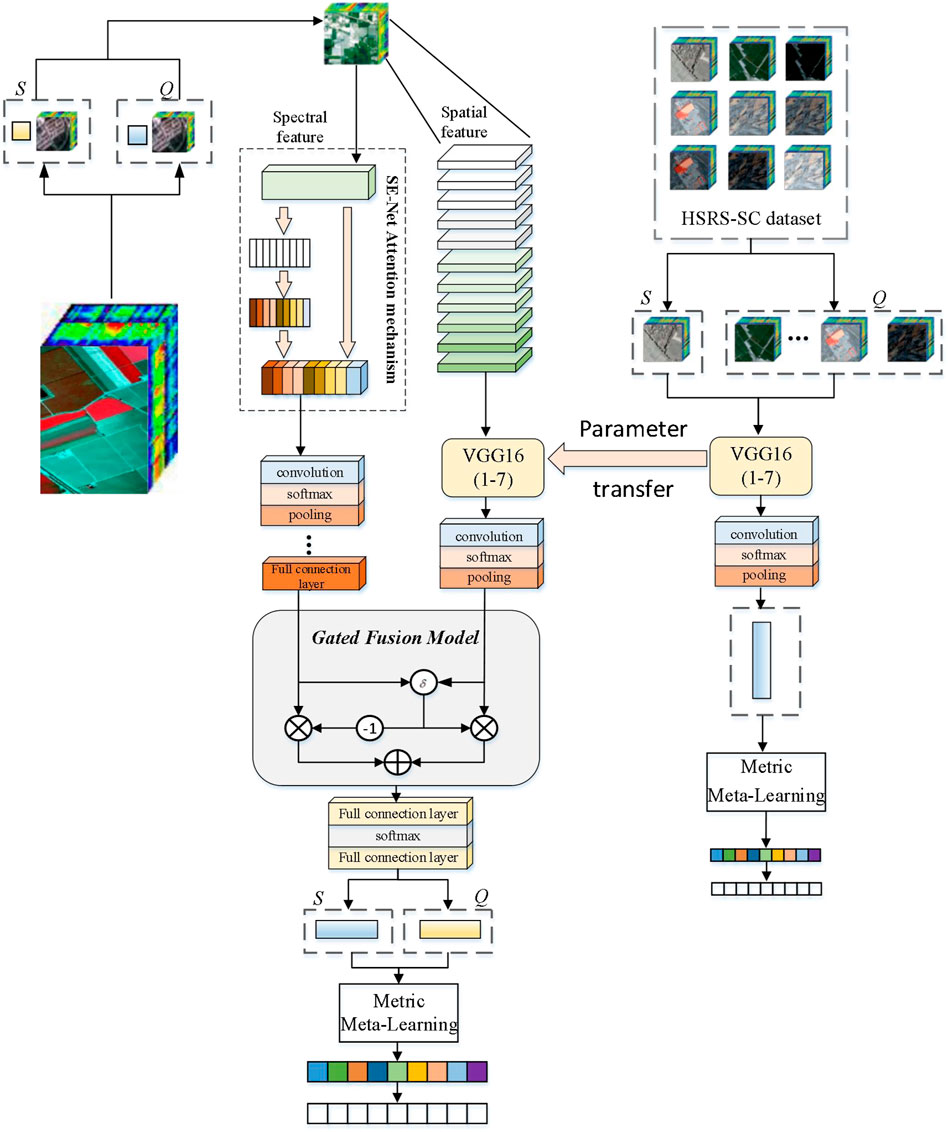
FIGURE 1. Joint spectral–spatial classification network based on the metric meta-learning model.

First, the hyperspectral dataset is divided into many different metatasks. Each task contains a small number of labeled samples (the support set) and unlabeled samples (the query set). Then, the support set and query set samples are simultaneously sent to the spectral–spatial joint transfer network module constructed to extract the spatial and spectral embedded features. The parameters in the spatial features are initialized by the network parameters trained on the HSRS-SC dataset to realize the transfer learning of spatial feature knowledge, which provides a new idea for hyperspectral image classification when training samples are insufficient. Then, the extracted spatial and spectral features are fused to gain more knowledge about general HSI features. Finally, the fused spectral–spatial features are sent into the metric meta-learning classification module and feature information is mapped into an embedding space by making full use of the metric space in the prior knowledge so that the model can achieve the effect of quickly and efficiently classifying the image categories.

2.1 Spatial–spectral feature extraction module combined with transfer learning

This section starts from the perspective of joint spatial–spectral features and aims at optimizing feature extraction and proposes a spatial–spectral joint transfer network. For HSI classification, spectral feature extraction exclusively leads to difficult interpretation of high-level semantic information on features of HSI scenes. It is shown that modeling through the synergy of spatial and spectral information can combine the spectral and spatial advantages of images to better reveal the proprieties of HSI. The two branches of the network extract spatial features and spectral features of HSI, respectively, and a channel attention mechanism is applied after extracting spectral features. This mechanism can strengthen the extracted features and make them more discriminative, thus improving the classification effect of HSI. After the spatial features and spectral features are extracted, the two features are combined by the gated fusion method. The gated fusion method can selectively fuse the spatial–spectral features for the classification of different positions, according to the feature appearance of the input image.

2.1.1 Spectral feature extraction combined with SE attention mechanisms

For the spectral feature extraction model, the network is configured with one 1-D convolutional layer, one spectral residual block, one 1-D convolutional layer, and one FC layer. SE-Net adds attention mechanisms to channels, including two key operations: squeeze and incentive. It can be observed that the module obtains the best weight value through autonomous learning, which is generally implemented by the neural network. A feature recalibration mechanism based on the network model is proposed, which enables the model to find some small amount of information that needs to be focused on in a large amount of data, thus avoiding a waste of computing power on unimportant information.

The input $X$ of any size is first given, then the input is mapped by $F_{tr}$, resulting in its special transformation into a feature map $U$ ($U\in {\mathrm{R}}^{H\times W\times C}$). The convolutional neural network is then used to construct a corresponding SE block, which is used to re-calibrate the features. The calibration step is to generate an embedded global distribution channel feature response and aggregate the features with a dimension size of $C\times H\times W$ to obtain a feature size of $C\times 1\times 1$ so that the layer closest to the input layer can obtain the global receptive field. After the squeeze operation, an excitation operation is performed, which is to re-input the new feature and aggregate a new weight generated by each channel, which will be mapped to $U$ again to obtain the final output $\stackrel{\sim }{X}$ combined with the weight.

2.1.2 Spatial feature extraction network combined with transfer learning

As shown in Figure 1, the three parts of spectral feature extraction, spatial feature extraction, and spectral–spatial feature extraction constitute the joint spatial–spectral feature extraction network. However, a meta-learning training strategy is used to learn the embedding feature space suitable for the HSRS-SC dataset. The pre-trained VGGNet’s first seven-layer structure and parameters are used to train the data on the target domain, and the parameters are transferred to the feature extraction model of the HSRS-SC dataset. Then, a CNN with 2D convolution, 2D max-pooling, and FC layers is designed to extract spatial features. The 2D convolution layer is followed by the BN layer, ReLU activation function, and maximum pooling. A batch normalization (BN) layer is added after the 2D convolutional layer to solve gradient disappearance and improve the generalization ability of the model. The activation function is added after the normalization layer. Finally, an FC layer is added to generate spatial feature vectors.

After the spatial features and spectral features are extracted, the two features are combined by the gated fusion method, which can selectively fuse the spectral–spatial features for the classification of different positions according to the feature appearance of the input image. Through gated fusion, the network can select a reasonable combination scheme for each pixel, enhance suitable features and suppress inappropriate features, and extract richer HSI feature information.

2.2 Metric meta-learning classification module

As shown in Figure 1, the obtained spectral–spatial feature vector used to be classified by comparing the distance of labeled samples and unlabeled samples based on metric element learning. The method in this paper is an improvement on the classic algorithm of metric-based meta-learning. The estimated metric function minimizes the difference between similar tasks, which maximizes the distance between dissimilar tasks and improves the efficiency of task processing. The known support samples $x_j$ and query samples $x_i$ generate the eigenvector sums of two sets of $E_{\phi }\left(x_i\right)$ and $E_{\phi }\left(x_j\right)$ through the spectral–spatial transfer network module, and then generate eigenvectors through splicing operation $C\left(*,*\right)$. The distance between samples can be used to obtain sample attributes ${\mathrm{C}\mathrm{o}\mathrm{n}}_i^j$ without using all the features of samples, which can make more effective use of HSI features and reduce the model’s dependence on training samples.

${\mathrm{C}\mathrm{o}\mathrm{n}}_i^j=C\left(E_{\phi }\left(x_i\right),E_{\phi }\left(x_j\right)\right).(1)$

${\mathrm{M}}_{\mathrm{\varphi }}$ is a neural network consisting of three regular convolutional layers. The first two convolution layers, with the size of 1 × 1 × 64, are followed by the Leaky-ReLU activation function for non-linear mapping. The sigmoid activation function is then used to output the similarity between samples, then the output feature vector is mapped to $M_{\varphi }$ and convolved by a convolutional layer. By analyzing the similarity between samples to obtain class $x_j$, feature vectors and relationship scores $m_{i,j}$ are generated xj.

In order to determine the label of the query sample, the feature mapping of each combination is input into $M_{\varphi }$ to generate a similarity, which is defined to indicate the similarity between any two embedded samples. The value of the output $m_{i,j}$ is a range of $\left[\mathrm{0,1}\right]$, in which the samples with high similarity scores are considered to be more similar.

$m_{i,j}=M_{\varphi }\left(C\left(E_{\phi }\left(x_i\right),E_{\phi }\left(x_j\right)\right)\right).(2)$

The comparison measurement model uses the mean squared error (MSE) loss function to calculate the relationship score and conduct training. When the training samples belong to the same category, the loss value is 1; otherwise, it is 0. The loss function is shown as follows: ${\left(m_{i,j}-\mathrm{l}\left(y_i==y_j\right)\right)}^2$

$\varphi ,\phi \leftarrow \underset{\varphi ,\phi }{\arg \mathit{min}}{\displaystyle \sum }_{x_i}.(3)$

3 Results

In order to prove the effectiveness of this method, classification experiments are carried out on public datasets, namely, Pavia University and Salinas datasets, and the transfer learning dataset selects the HSRS-SC dataset. All experiments were conducted using the Intel (R) Xeon (R) 4208 CPU @ 2.10 GHz processor and Nvidia GeForce RTX 2080Ti graphics card. The number of training iterations is set to 1,000. For each training iteration, K is set to 1 and N is set to 19, which is the number of categories in the HSI dataset; that is, 1 labeled sample and 19 unlabeled samples were selected randomly to form a training set for model training. In addition, the model in this paper is optimized using Adam, and the learning rate is set to 0.001.

3.1 Comparison with state-of-the-art methods

In order to evaluate the effectiveness of the meta-learning method, this paper compares the meta-learning method with deep learning and few-shot supervised learning methods including extended morphological profile support vector machine (EMP-SVM) [16], deep convolutional neural network (DCNN) [17], residual network (ResNet) [18], and current few-shot learning methods including relation network (RLNet) [19], deep cross-domain few-shot learning (DCFSL) [20], and heterogeneous few-shot learning (HFSL) [21]. In order to ensure the fairness of the experiment, this paper randomly selects five labeled samples in each type of HSI dataset as the supervised samples. All experiments were performed 10 times to remove the effect of random sampling. Tables 1, 2 show the accuracy values of OA, AA, and kappa of Pavia University and Salinas datasets.

TABLE 1

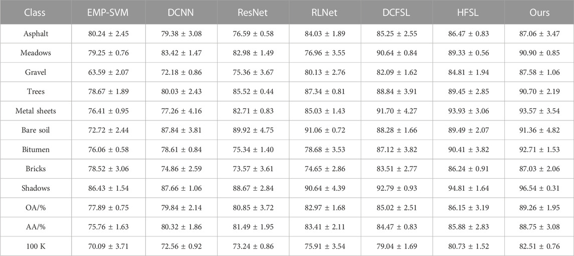
TABLE 1. Classification results of different methods on the Pavia University dataset.

TABLE 2

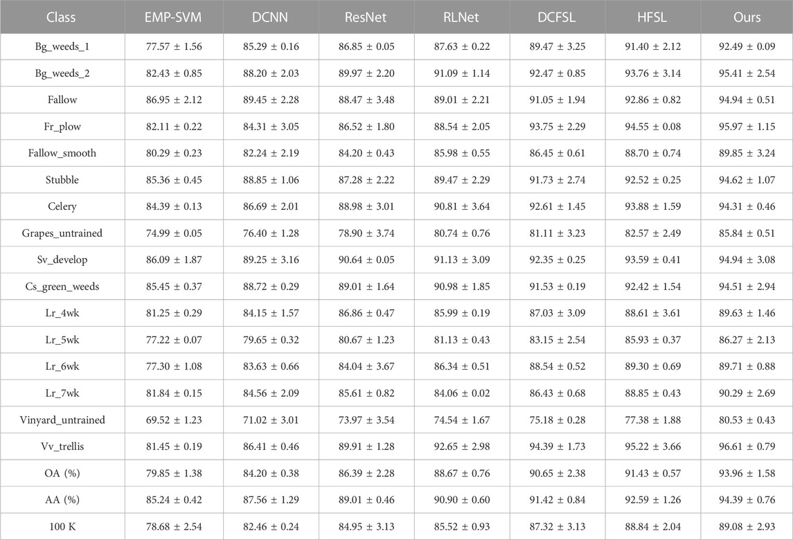
TABLE 2. Classification results of different methods on the Salinas dataset.

From Tables 1, 2, it can be seen that the proposed method in this paper achieves almost the highest classification accuracy in each class. In particular, it improves the classification accuracy more for classes with lower heights, such as the asphalt road class and the grass class in the Pavia University dataset. As shown in Table 1, the OA value of the Pavia University dataset is as high as 82.96%, and compared with EMP-SVM, DCNN, ResNet, RLNet, DCFSL, and HFSL, it has increased by 11.37%, 9.42%, 8.41%, 6.29%, 4.24%, and 3.11%, respectively. These results demonstrate the superiority of meta-learning methods in HSI classification. For categories that other methods cannot accurately classify, such as gravel, bare soil, asphalt, and bricks, the meta-learning method can obtain more accurate classification results, further demonstrating its effectiveness.

Figures 2, 3, respectively, show the HSI ground truth maps and the false color image maps of the classification results. In the small-sample ground objects, the error features such as gravel and bricks have been significantly improved, and it can correct various types of ground objects with a small number of training samples.

FIGURE 2

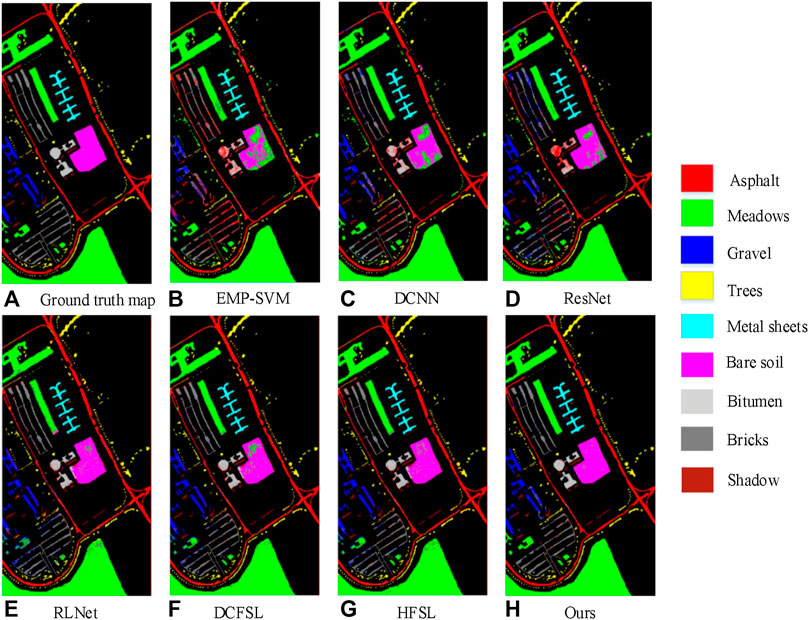
FIGURE 2. Classification maps of the Pavia University dataset. (A) ground truth; (B) EMP-SVM; (C) DCNN; (D) ResNet; (E) RLNet; (F) DCFSL; (G) HFSL; (H) Ours.

FIGURE 3

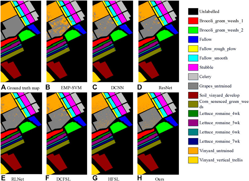
FIGURE 3. Classification maps of the Salinas dataset. (A) ground truth; (B) EMP-SVM; (C) DCNN; (D) ResNet; (E) RLNet; (F) DCFSL; (G) HFSL; (H) Ours.

In Figure 3, the SVM algorithm only considers the spectral feature, and the misclassification rate for Vinyard_untrained and Grapes_untrained is higher. DCNN and other deep learning algorithms are better than SVM in the classification of Vinyard_untrained and Grapes_untrained, which shows that it has good feature extraction ability in large-scale landforms. On this dataset, the meta-learning algorithm has greatly improved compared with other algorithms, and the classification effect is the best.

4 Discussion

In order to verify the HSI classification framework based on model transfer, the influence of different datasets on the classification results in transfer learning was studied to construct the optimal classification framework. Figure 4 shows the results of classification using different datasets for transfer learning, where CP means the center of Pavia dataset, SA means the Salinas dataset, HS means the HSRS-SC dataset, and IM means the natural image dataset ImageNet. Through the visualization of experimental data, it can be found that the model-based transfer learning method is effective. As shown in Figure 4F, the classification result obtained by using the HSRS-SC as the source dataset is better than the other three types and is closer to the ground truth map in terms of spatial correlation and completeness, especially the soil class. Rich information on source domain data facilitates the learning of pre-trained models. By using the HSRS-SC dataset to train the model, the obtained model has a stronger feature extraction ability and is able to learn more general features rather than features limited to a specific dataset so that the migration of the pre-trained model to the target domain can better adapt to the new learning task well.

FIGURE 4

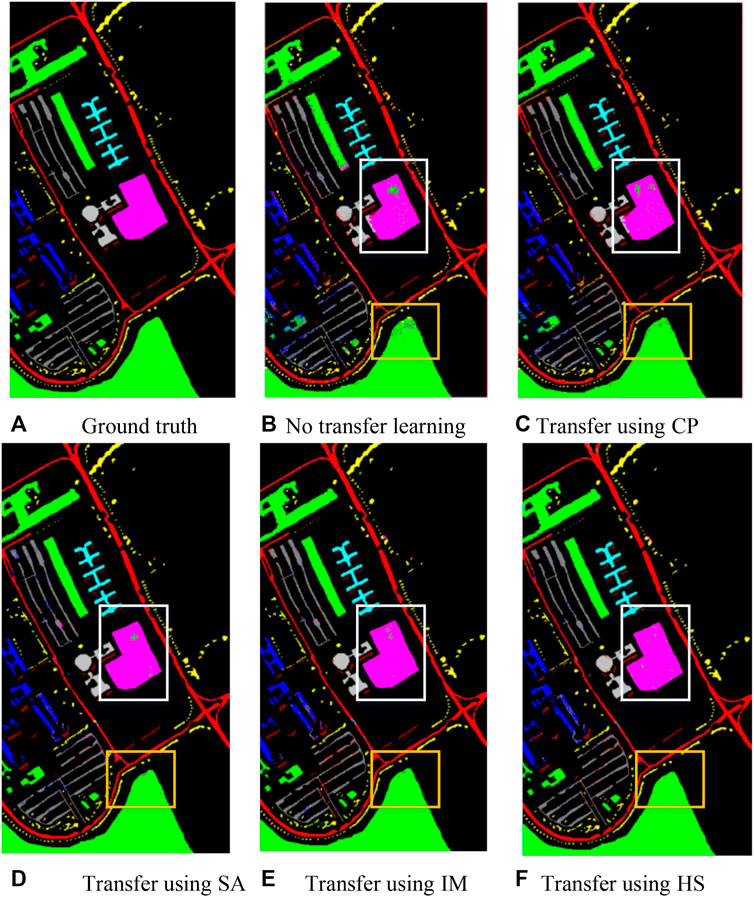
FIGURE 4. Classification visualization result diagram using different transfer datasets. (A) Ground truth; (B) No transfer learning; (C) Transfer using CP; (D) Transfer using SA; (E) Transfer using IM; (F) Transfer using HS.

5 Conclusion

In order to improve the classification accuracy of hyperspectral images, this paper designs a spatial–spectral joint transfer classification network based on metric meta-learning. Furthermore, to combine the spectral and spatial superiority of HSI, a joint spatial–spectral transfer learning network module is proposed in this paper, which can extract finer HSI features and capture cross-dimensional and spatial interaction information. The experimental results on two publicly available HSI datasets show that the meta-learning method proposed in this paper is more competitive and outperforms other classical methods and existing few-shot learning methods. In the future, we will study model compression and pruning to reduce the complexity of the proposed model and improve real-time performance without affecting the classification ability.

Data availability statement

The original contributions presented in the study are included in the article/Supplementary Material; further inquiries can be directed to the corresponding author.

Author contributions

All authors listed have made a substantial, direct, and intellectual contribution to the work and approved it for publication.

Funding

This work was funded by the Reserved Leaders of Heilongjiang Provincial Leading Talent Echelon of 2021, the High-end Foreign Expert’s Introduction Program (G2022012010L), and the Key Research and Development Program Guidance Project (GZ20220123).

Conflict of interest

The authors declare that the research was conducted in the absence of any commercial or financial relationships that could be construed as a potential conflict of interest.

Publisher’s note

All claims expressed in this article are solely those of the authors and do not necessarily represent those of their affiliated organizations, or those of the publisher, the editors, and the reviewers. Any product that may be evaluated in this article, or claim that may be made by its manufacturer, is not guaranteed or endorsed by the publisher.

References

1. Tong QX, Zhang B, Zhang LF. Current progress of hyperspectral remote sensing in China. J Remote Sensing (2016) 20(5):689–707. doi:10.11834/jrs.20166264

CrossRef Full Text | Google Scholar

2. Julie T, Raphael DA, Alexandre M, Defourny P. Survey of hyperspectral earth observation applications from space in the sentinel-2 context. Remote Sensing (2018) 10(3):157. doi:10.3390/rs10020157

CrossRef Full Text | Google Scholar

3. Chen Y, Lin Z, Zhao X, Wang G, Gu Y. Deep learning-based classification of hyperspectral data. IEEE J.-STARS (2014) 7:2094–107. doi:10.1109/jstars.2014.2329330

CrossRef Full Text | Google Scholar

4. Li T, Zhang J, Zhang Y. Classification of hyperspectral image based on deep belief networks. In: 2014 IEEE International Conference on Image Processing (ICIP); 27-30 October 2014; Paris, France (2014). p. 5132–6. doi:10.1109/ICIP.2014.7026039

CrossRef Full Text | Google Scholar

5. Makantasis K, Karantzalos K, Doulamis A, Doulamis N. Deep supervised learning for hyperspectral data classification through convolutional neural networks. In: 2015 IEEE International Geoscience and Remote Sensing Symposium (IGARSS); 26-31 July 2015; Milan, Italy (2015). p. 4959–62. doi:10.1109/IGARSS.2015.7326945

CrossRef Full Text | Google Scholar

6. Chen Y, Jiang H, Li C, Jia X, Ghamisi P. Deep feature extraction and classification of hyperspectral images based on convolutional neural networks. IEEE Trans. Geosci. Remo. Sen. (2016) 54:6232–51. doi:10.1109/tgrs.2016.2584107

CrossRef Full Text | Google Scholar

7. Wang L, Peng J, Sun W. Spatial-spectral squeeze-and-excitation residual network for hyperspectral image classification. Remote Sens (2019) 11:884–90. doi:10.3390/rs11070884

CrossRef Full Text | Google Scholar

8. Zhong Z, Li J, Luo Z, Chapman M. Spectral-spatial residual network for hyperspectral image classification: A 3-d deep learning framework. IEEE T Geosci Remote (2017) 56:847–58. doi:10.1109/tgrs.2017.2755542

CrossRef Full Text | Google Scholar

9. Paoletti ME, Haut JM, Ez-Beltran R, Plaza J, Plaza AJ, Pla F. Deep pyramidal residual networks for spectral-spatial hyperspectral image classification. IEEE T Geosci Remote (2018) 57:740–54. doi:10.1109/tgrs.2018.2860125

CrossRef Full Text | Google Scholar

10. Santoro A, Bartunov S, Botvinick M, Wierstra D, Lillicrap T. One-shot learning with memory-augmented neural networks. In: International Conference on Machine Learning; 19, May 2016; Sydney, Australia (2016).

Google Scholar

11. Munkhdalai T, Yu H. Meta networks. In: International Conference on Machine Learning; Sydney, Australia (2017). p. 2554–63.

Google Scholar

12. Vinyals O, Blundell C, Lillicrap T, Kavukcuoglu K, Wierstra D, et al. Matching networks for one shot learning. Adv Neural Inf Process Syst (2016) 29:3630–8. doi:10.48550/arXiv.1606.04080

CrossRef Full Text | Google Scholar

13. Snell J, Swersky K, Zemel RS. Prototypical networks for few-shot learning. Neural Inf Process Syst (2017) 1703:05175. doi:10.48550/arXiv.1703.05175

CrossRef Full Text | Google Scholar

14. Finn C, Abbeel P, Levine S. Model-agnostic meta-learning for fast adapt ation of deep networks. In: International Conference on Machine Learning; Sydney, Australia (2017). p. 1126–35.

Google Scholar

15. Rusu AA, Rao D, Sygnowski J, Vinyals O, Pascanu R, Osindero S Meta-learning with latent embedding optimization. In: 7th International Conference on Learning Representations; New Orleans, LA, USA (2018). p. 671–83.

Google Scholar

16. Gu YF, Liu TZ, Jia XP, Benediktsson JA, Chanussot J. Nonlinear multiple kernel learning with multiple-structure-element extended morphological profiles for hyperspectral image classification. IEEE Trans Geosci Remote Sensing (2016) 54(6):3235–47. doi:10.1109/tgrs.2015.2514161

CrossRef Full Text | Google Scholar

17. Song W, Li S, Fang L, Lu T Hyperspectral image classification with deep feature fusion network[J]. IEEE Trans Geosci Remote Sensing (2018) 56(6):1–12. doi:10.1109/TGRS.2018.2794326

CrossRef Full Text | Google Scholar

18. Paoletti ME, Haut JM, Plaza J, Plaza A A new deep convolutional neural network for fast hyperspectral image classification[J]. Isprs J Photogrammetry Remote Sensing (2017) 145PA(NOV):120–47. doi:10.1016/j.isprsjprs.2017.11.021

CrossRef Full Text | Google Scholar

19. Deng B, Shi D. Relation network for hyperspectral image classification. In: 2019 IEEE International Conference on Multimedia and Expo Workshops (ICMEW); 08-12 July 2019; Shanghai, China. IEEE (2019).

CrossRef Full Text | Google Scholar

20. Li Z, Liu M, Chen Y, Xu Y, Li W, Du Q. Deep cross-domain few-shot learning for hyperspectral image classification. IEEE Trans Geosci Remote Sensing (2021) 60(99):1–18. doi:10.1109/tgrs.2021.3057066

CrossRef Full Text | Google Scholar

21. Wang Y, Liu M, Yang Y, Li Z, Du Q, Chen Y, et al. Heterogeneous few-shot learning for hyperspectral image classification. IEEE Geosci Remote Sens Lett (2022) 19:1–5. doi:10.1109/lgrs.2021.3117577

CrossRef Full Text | Google Scholar