Acoustic scattering of a pair of rigid spheroids based on the T-matrix method

1 Introduction

The study of underwater target acoustic scattering gains attentions from researchers, and the relative research studies are widely applied in engineering practices such as underwater target detection, positioning, imaging, and underwater communication. The mechanism of multiple-target acoustic scattering is more complex than that of single-target scattering due to the existence of multiple scattering. In this study, a pair of rigid spheroids is chosen as the target to investigate the multiple acoustic scattering characteristics.

In the past decades, a series of numerical and analytical methods are proposed to solve the underwater acoustic scattering problem. Numerical methods such as the finite element method (FEM) and boundary element method (BEM) can solve acoustic scattering problems under complex conditions [1–3]. Recently, various extended methods, like the smooth finite element method and meshfree method [4–7], are proposed to solve the underwater acoustic scattering issues. However, the computational efficiency of those numerical methods decreases as the frequency increases because of the requirement of very dense meshes. Compared to the numerical methods, the analytical method can provide precise solutions with a faster convergence speed. In addition, the physical understanding of the acoustic scattering wave can be explained by the analytical solutions. Rayleigh first derived the Bessel–Legendre series (mathematical) solution for the acoustic scattering of a sphere by the variable separation method. However, his works are only competent to cases with small non-dimensional frequencies $ka$ [8]. Based on Rayleigh’s work, various extended analytical methods, like the partial wave series (PWS) method and Sommerfeld–Watson transformation (SWT), are proposed to obtain the mathematical expressions of acoustic scattering of the single simple target (such as the sphere and circular cylinder) [9–11]. Záviška proposed the multipole method to solve the two-dimensional multiple scattering by a series of circular cylinders [12]. Eyges extended the multipole method to the multiple scattering of two spheres [13]. The key to the multipole method is the addition theorems of the spherical basis functions which transform the multiple scattering fields of different targets to a field with a uniform origin [14, 15]. Gabrielli derived the analytical solutions to the acoustic scattering problems of two spheres using the symmetry properties, which are widely used in quantum physics [15, 16]. However, there are some limitations to analytical methods in solving the acoustic scattering of non-spherical targets in the spherical coordinate system. Consequently, the semi-analytical method is applied to study the far-field acoustic scattering of a pair of rigid spheroids.

The T-matrix method, a typical semi-analytical method, is first proposed by Waterman for electromagnetic scattering problems [17] and later extended to the acoustic scattering field [18]. The T-matrix method is defined as the semi-analytical method derived from the Helmholtz integral equation and null-field theory, and the infinite matrix needs to be truncated. The crux of the T-matrix method is to expand all the field quantities by a set of orthogonal basis functions and solve the unknown expansion coefficients. In addition, the T-matrix method is suitable for the acoustic scattering problem with arbitrary incidence and scattering angles. Peterson derived the T-matrix expression for multi-target scattering based on the addition theorems of spherical basis functions and calculates the numerical result of a pair of identical spheres under the plane wave incidence [19]. Most of the published literature works focus on the acoustic scattering of a pair of spheres and spheroids with small aspect ratios (i.e., the ratio of the polar radius to equatorial radius is less than 2). However, it is important to study the acoustic scattering mechanism of a pair of rigid oblate spheroids and prolate spheroids, which are extensively used in hydrodynamics and underwater engineering.

In this work, the addition theorems are embedded in the T-matrix method to investigate the underwater far-field acoustic scattering characteristics of a pair of rigid spheroids with different aspect ratios ensonified by plane waves at different angles. The propagation paths of the returning backscattering waves from a pair of rigid spheres are analyzed by using the geometric and numerical method in the time domain. The structure of this work is as follows: In Section 2, acoustic scatterings of a single rigid spheroid are considered by the traditional T-matrix method; in addition, the addition theorems are embedded in the T-matrix method to investigate the scatterings of a pair of rigid spheroids. In Section 3, some numerical experiments are carried out to verify the accuracy and convergence of the T-matrix method for the acoustic scattering of a pair of rigid spheroids. Furthermore, the effects of the separation distance between spheroids, aspect ratios, non-dimensional frequencies, and incidence angles of the plane wave on the acoustic scattering of a pair of rigid spheroids are investigated, while conclusions are provided in Section 4.

2 T-matrix method

In this section, a rigid spheroid and a spheroid pair are considered. The acoustic scatterings of such models under plane wave incidence at an arbitrary angle are investigated using the T-matrix method.

2.1 For a rigid spheroid

As shown in Figure 1, a rigid rotation spheroid with the polar radius $b$ (distance from the center point to the endpoint of the spheroid located in the rotation axis $Oz$) and equatorial radius $a$ is positioned in an ideal fluid medium with density $\rho$ and sound velocity $c$. The angle between the incident plane wave P and axis $Oz$ is ${\theta }_i$. The surface shape function $S\left(\theta \right)$ of the spheroid is only related to the polar angle $\theta$, such that

$S\left(\theta \right)={\left({\cos }^2\theta /b^2+{\sin }^2\theta /a^2\right)}^{-1/2}.(1)$

FIGURE 1

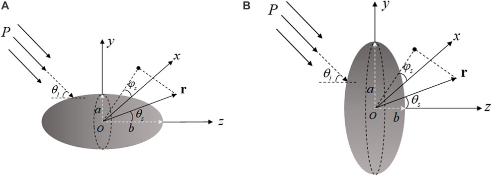
FIGURE 1. Geometry model for the acoustic scattering of a rigid (A) prolate and (B) oblate spheroid.

The entire wave field can be constructed by the scalar velocity potential because the wave field exists only in the ideal fluid medium. For convenience, in what follows, the monochromatic time factor $\exp \left(-i\omega t\right)$ of all velocity potentials is omitted. The total wave field $\mathrm{\Phi }\left(\mathbf{r}\right)$ is the sum of the incident field ${\mathrm{\Phi }}_i\left(\mathbf{r}\right)$ and scattering field ${\mathrm{\Phi }}_s\left(\mathbf{r}\right)$:

$\mathrm{\Phi }\left(\mathbf{r}\right)={\mathrm{\Phi }}_i\left(\mathbf{r}\right)+{\mathrm{\Phi }}_s\left(\mathbf{r}\right).(2)$

All of the aforementioned velocity potentials satisfy the Helmholtz equation:

$\left({\nabla }^2+k^2\right)\left(\begin{array}{l}\mathrm{\Phi }\left(\mathbf{r}\right)\\ {\mathrm{\Phi }}_i\left(\mathbf{r}\right)\\ {\mathrm{\Phi }}_s\left(\mathbf{r}\right)\end{array}\right)=0,(3)$

where $k=\omega /c$ is the wave number. Waterman discussed the aforementioned three field functions in detail [18]. The outer surface S of the ellipsoid is smooth, so that the Poincare–Huygens principle and Gauss theorem can be applied. The Helmholtz integral representation equation can be expressed as

${\mathrm{\Phi }}_i\left(\mathbf{r}\right)+{\int }_S\left[{\mathrm{\Phi }}_{+}\mathbf{n}\cdot \nabla g\left(\mathbf{r},{\mathbf{r}}^{\prime }\right)-\left(\mathbf{n}\cdot {\nabla }_{+}\mathrm{\Phi }\right)g\left(\mathbf{r},{\mathbf{r}}^{\prime }\right)\right]\mathrm{d}S=\left\{\begin{array}{l}\mathrm{\Phi }\left(\mathbf{r}\right)\mathbf{r}\mathrm{o}\mathrm{u}\mathrm{t}\mathrm{s}\mathrm{i}\mathrm{d}\mathrm{e}S\\ 0\mathbf{r}\mathrm{i}\mathrm{n}\mathrm{s}\mathrm{i}\mathrm{d}\mathrm{e}S,\end{array}\right.(4)$

where ${\mathrm{\Phi }}_{+}$ is the velocity potential on the outer surface of the spheroid. $\mathbf{n}\cdot {\nabla }_{+}\mathrm{\Phi }$ denotes the normal velocity on the outer surface of the spheroid. $g\left(\mathbf{r},{\mathbf{r}}^{\prime }\right)$ is the free-field Green’s function, which can be expressed as

$g\left(\mathbf{r},{\mathbf{r}}^{\prime }\right)=\exp \left(ik\left|\mathbf{r}-{\mathbf{r}}^{\prime }\right|\right)/\left(k\left|\mathbf{r}-{\mathbf{r}}^{\prime }\right|\right).(5)$

The crucial point is to expand the whole field quantities with a set of orthogonal basis functions and solve the corresponding unknown coefficients. The scalar spherical basis function is expressed as

$\begin{array}{l}{\mathrm{\Phi }}_{nm\sigma }\left(\mathbf{r}\right)=h_n^{\left(1\right)}\left(kr\right)Y_{nm\sigma }\left(\theta ,\phi \right)\\ =h_n\left(kr\right){\xi }_{nm}^{\prime }{P}_n^m\left(\cos \theta \right)\left(\begin{array}{l}\cos \left(m\phi \right),\sigma =e\\ \sin \left(m\phi \right),\sigma =o\end{array}\right)\end{array},(6)$

where $P_n^m\left(\cos \theta \right)$ is the associated Legendre function of order $n$ and rank $m$. The azimuthal parity index $\sigma$ is either even or odd. $h_n^{\left(1\right)}\left(kr\right)$ is a spherical Hankel function of the first kind. The normalization coefficients ${\xi }_{nm}^{\prime }$ can be expressed as

${\xi }_{nm}^{\prime }={\left[{\epsilon }_m\left(2n+1\right)\left(n-m\right)!\right]}^{1/2}\times {\left[4\pi \left(n+m\right)!\right]}^{-1/2},(7)$

with ${\epsilon }_m=\left\{\begin{array}{l}1,m=0\\ 2,m\ne 0\end{array}\right.$. The value range of the order index is $n=\mathrm{0,1},\cdots ,\infty$, and the rank index $m$ takes the integer values $m=\mathrm{0,1},\cdots ,n$.

The incident and scattered field can be expanded into the form of the weighted sum of the scalar basis function with the expanded coefficients. The regular spherical basis function, denoted by $\mathrm{R}\mathrm{e}{\mathrm{\Phi }}_{nm\sigma }$, is obtained by substituting the first-kind spherical Bessel function $j_n\left(kr\right)$ for $h_n^{\left(1\right)}\left(kr\right)$ into Eq. 6. Therefore, the incident and scattered fields can be expanded as

${\mathrm{\Phi }}_i\left(\mathbf{r}\right)={\displaystyle \sum _{nm\sigma }}{a}_{nm\sigma }\mathrm{R}\mathrm{e}{\mathrm{\Phi }}_{nm\sigma }\left(\mathbf{r}\right),(8)$

${\mathrm{\Phi }}_s\left(\mathbf{r}\right)={\displaystyle \sum _{nm\sigma }}{f}_{nm\sigma }{\mathrm{\Phi }}_{nm\sigma }\left(\mathbf{r}\right),(9)$

where ${\displaystyle \sum _{nm\sigma }}={\displaystyle \sum _{n=0}^{\infty }}{\displaystyle \sum _{m=0}^n}{\displaystyle \sum _{\sigma }}$ is the triple summation symbol, $a_{nm\sigma }$ denotes the expanded coefficient of the incident field, and $f_{nm\sigma }$ denotes the unknown expanded coefficient of the scattering field. For a plane harmonic wave, the expanded coefficient is

$a_{nm\sigma }=4\pi {\xi }_{nm}^{\prime }{i}^n{P}_n^m\left(\cos {\theta }_i\right)\left(\begin{array}{l}\cos \left(m{\phi }_i\right),\sigma =e\\ \sin \left(m{\phi }_i\right),\sigma =o\end{array}\right).(10)$

Furthermore, the free-field Green’s function $g\left(\mathbf{r},{\mathbf{r}}^{\prime }\right)$ can be expanded using the spherical basis function as

$g\left(\mathbf{r},{\mathbf{r}}^{\prime }\right)={\displaystyle \sum _{nm\sigma }}ik{\mathrm{\Phi }}_{nm\sigma }\left(r_{>}\right)\mathrm{R}\mathrm{e}{\mathrm{\Phi }}_{nm\sigma }\left(r_{<}\right),(11)$

where $r_{>}=\left\{\begin{array}{l}r,r>r^{\prime }\\ r^{\prime },r<r^{\prime }\end{array}\right.$ and $r_{<}=\left\{\begin{array}{l}r,r<r^{\prime }\\ r^{\prime },r>r^{\prime }\end{array}\right.$. $r^{\prime }$ is the modulus of the point ${\mathbf{r}}^{\prime }$ on the surface $S$ of the spheroid. $r$ is the modulus of the field point $\mathbf{r}$. The expanded expression of the unknown surface field ${\mathrm{\Phi }}_{+}$ is

${\mathrm{\Phi }}_{+}\left({\mathbf{r}}^{\prime }\right)={\displaystyle \sum _{nm\sigma }}{\alpha }_{nm\sigma }\mathrm{R}\mathrm{e}{\mathrm{\Phi }}_{nm\sigma }\left({\mathbf{r}}^{\prime }\right),(12)$

where ${\alpha }_{nm\sigma }$, which is omitted in the process of deriving the T-matrix, is the expanded coefficient of the unknown surface field.

For a rigid spheroid, the boundary of the spheroid at $\mathbf{r}=S\left(\theta \right)$ satisfies the Neumann boundary condition:

$\mathbf{n}\cdot {\nabla }_{+}\mathrm{\Phi }\left(\mathbf{r}\right){|}_{\mathbf{r}=S\left(\theta \right)}=0.(13)$

Substituting Eqs 6–13 into Eq. 4 yields

$i{\displaystyle \sum _{n^{\prime }{m}^{\prime }{\sigma }^{\prime }}}{Q}_{nm\sigma ,n^{\prime }{m}^{\prime }{\sigma }^{\prime }}{\alpha }_{n^{\prime }{m}^{\prime }{\sigma }^{\prime }}=-a_{nm\sigma },(14)$

$i{\displaystyle \sum _{n^{\prime }{m}^{\prime }{\sigma }^{\prime }}}\mathrm{R}\mathrm{e}{Q}_{nm\sigma ,n^{\prime }{m}^{\prime }{\sigma }^{\prime }}{\alpha }_{n^{\prime }{m}^{\prime }{\sigma }^{\prime }}=f_{nm\sigma },(15)$

where

$Q_{nm\sigma ,n^{\prime }{m}^{\prime }{\sigma }^{\prime }}=k{\int }_S\mathrm{R}\mathrm{e}{\mathrm{\Phi }}_{n^{\prime }{m}^{\prime }{\sigma }^{\prime }}\left({\mathbf{r}}^{\prime }\right)\mathbf{n}\cdot \nabla {\mathrm{\Phi }}_{nm\sigma }\left({\mathbf{r}}^{\prime }\right)\mathrm{d}S.(16)$

The detailed expression of $Q_{nm\sigma ,n^{\prime }{m}^{\prime }{\sigma }^{\prime }}$ is obtained by substituting Eq. 6 into Eq. 16:

$\begin{array}{l}{Q}_{nm\sigma ,n^{\prime }{m}^{\prime }{\sigma }^{\prime }}={\int }_0^{\pi }{\xi }_{n^{\prime }{m}^{\prime }}^{\prime }{j}_{n^{\prime }}\left(kr\right)P_{n^{\prime }}^{m^{\prime }}\left(\cos \theta \right){\xi }_{nm}\times \left[\frac{\partial h_n\left(kr\right)}{\partial r}{P}_n^m\left(\cos \theta \right)-\right.\frac{r_{\theta }}{r^2}{h}_n\left(kr\right)\\ \left.\times \frac{\partial P_n^m\left(\cos \theta \right)}{\partial \theta }\right]\times r^2\sin \theta \mathrm{d}\theta {\int }_0^{2\pi }\left(\begin{array}{l}\cos m^{\prime }\phi \\ \sin m^{\prime }\phi \end{array}\right)\left(\begin{array}{l}\cos m\phi \\ \sin m\phi \end{array}\right)\mathrm{d}\phi \end{array},(17)$

where $r_{\theta }=\partial r\left(\theta \right)/\partial \theta$ and $r\left(\theta \right)=S\left(\theta \right)$. In the expression of the Q-matrix, the symmetry of the scatterer leads to certain elements in the Q-matrix becoming zero. In this study, the rotational symmetry of the spheroid makes the Q-matrix block diagonal of the submatrices, and thus, the computation can be simplified.

From Eqs 14, 15, the relationship between scattering and incident expanded coefficients can be expressed as

$f_{nm\sigma }=T{a}_{nm\sigma },(18)$

where the transition matrix $T$, showing the influence of the geometry of the spheroid, the incident angle, and the frequency of the plane wave [20, 21], is expressed as

$T=-\left(\mathrm{R}\mathrm{e}Q\right)Q^{-1}.(19)$

2.2 For a pair of rigid spheroids

In this part, the formula of the T-matrix method for a pair of rigid spheroids immersed in the idea fluid is derived. The geometry of the configuration to be considered is shown in Figure 2. The formula of the T-matrix method for a pair of rigid spheroids is derived exactly like Eq. 4:

${\mathrm{\Phi }}_i\left(\mathbf{r}\right)+{\int }_{S_1+S_2}\left[{\mathrm{\Phi }}_{+}\mathbf{n}\cdot \nabla g\left(\mathbf{r},{\mathbf{r}}^{\prime }\right)-\left(\mathbf{n}\cdot {\nabla }_{+}\mathrm{\Phi }\right)g\left(\mathbf{r},{\mathbf{r}}^{\prime }\right)\right]\mathrm{d}S=\left\{\begin{array}{l}\mathrm{\Phi }\left(\mathbf{r}\right)\mathbf{r}\mathrm{o}\mathrm{u}\mathrm{t}\mathrm{s}\mathrm{i}\mathrm{d}\mathrm{e}{S}_1\mathrm{a}\mathrm{n}\mathrm{d}{S}_2\\ 0\mathbf{r}\mathrm{i}\mathrm{n}\mathrm{s}\mathrm{i}\mathrm{d}\mathrm{e}{S}_1\mathrm{o}\mathrm{r}{S}_2.\end{array}\right.(20)$

FIGURE 2

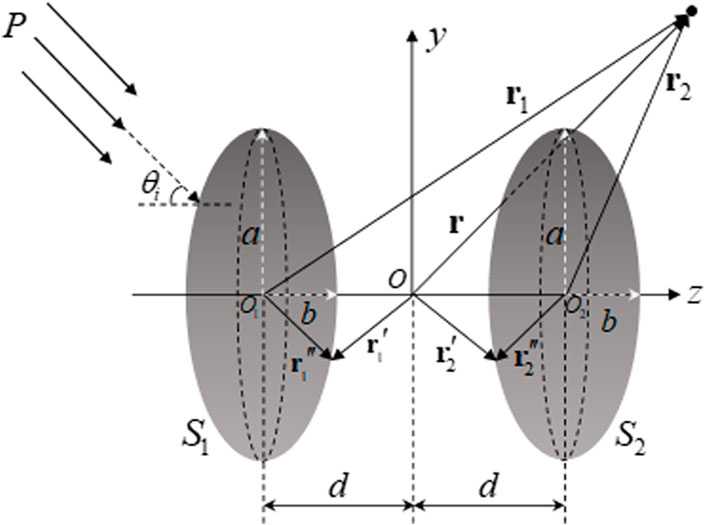
FIGURE 2. Geometry model for the acoustic scattering of a pair of rigid spheroids.

The incident field ${\mathrm{\Phi }}_i\left(\mathbf{r}\right)$ and the free-field Green’s function $g\left({\mathbf{r},\mathbf{r}}^{\prime }\right)$ need to be expanded at origins $O_1$ and $O_2$ to obtain the Q-matrix of each of the spheroids, which are analogous to Eq. 16. When the field point $\mathbf{r}$ is located inside $S_1$,

$\mathbf{r}={\mathbf{r}}_1-\mathbf{d},{\mathbf{r}}^{\prime }={\mathbf{r}}_{\mathbf{1}}^{\prime },\mathbf{r}-{\mathbf{r}}_1^{\prime }={\mathbf{r}}_1-{\mathbf{r}}_1^{″},\mathbf{r}-{\mathbf{r}}_2^{\prime }={\mathbf{r}}_1-\left({\mathbf{r}}_2^{″}+2\mathbf{d}\right),(21)$

where $\mathbf{d}=\overrightarrow{O_{1}O}=\overrightarrow{O{O}_2}$. According to Eq. 11, Green’s functions $g\left(\mathbf{r},{\mathbf{r}}_1^{\prime }\right)$ and $g\left(\mathbf{r},{\mathbf{r}}_2^{\prime }\right)$ can be written as

$g\left(\mathbf{r},{\mathbf{r}}_1^{\prime }\right)={\displaystyle \sum _{nm\sigma }}ik{\mathrm{\Phi }}_{nm\sigma }\left({\mathbf{r}}_1^{″}\right)\mathrm{R}\mathrm{e}{\mathrm{\Phi }}_{nm\sigma }\left({\mathbf{r}}_1\right),(22)$

$g\left(\mathbf{r},{\mathbf{r}}_2^{\prime }\right)={\displaystyle \sum _{nm\sigma }}ik{\mathrm{\Phi }}_{nm\sigma }\left({\mathbf{r}}_2^{″}+2\mathbf{d}\right)\mathrm{R}\mathrm{e}{\mathrm{\Phi }}_{nm\sigma }\left({\mathbf{r}}_1\right).(23)$

From Eqs 8, 21, where $\mathbf{r}={\mathbf{r}}_1-\mathbf{d}$, the incident fields can be expressed as

${\mathrm{\Phi }}_i\left(\mathbf{r}\right)={\displaystyle \sum _{nm\sigma }}{a}_{nm\sigma }\mathrm{R}\mathrm{e}{\mathrm{\Phi }}_{nm\sigma }\left({\mathbf{r}}_1-\mathbf{d}\right).(24)$

The addition theorems of the spherical basis functions are used in Eqs 23, 24. The translation properties are as follows [22, 23]:

$\begin{array}{l}\mathrm{R}\mathrm{e}{\mathrm{\Phi }}_{nm\sigma }\left(\mathbf{r}+\mathbf{d}\right)={\displaystyle \sum _{n^{\prime }{m}^{\prime }{\sigma }^{\prime }}}{\widehat{R}}_{nm\sigma ,n^{\prime }{m}^{\prime }{\sigma }^{\prime }}\left(\mathbf{d}\right)\mathrm{R}\mathrm{e}{\mathrm{\Phi }}_{n^{\prime }{m}^{\prime }{\sigma }^{\prime }}\left(\mathbf{r}\right),\\ {\mathrm{\Phi }}_{nm\sigma }\left(\mathbf{r}+\mathbf{d}\right)=\left\{\begin{array}{l}{\displaystyle \sum _{n^{\prime }{m}^{\prime }{\sigma }^{\prime }}}{\widehat{R}}_{nm\sigma ,n^{\prime }{m}^{\prime }{\sigma }^{\prime }}\left(\mathbf{d}\right){\mathrm{\Phi }}_{n^{\prime }{m}^{\prime }{\sigma }^{\prime }}\left(\mathbf{r}\right),\left|\mathbf{r}\right|>\left|\mathbf{d}\right|,\\ {\displaystyle \sum _{n^{\prime }{m}^{\prime }{\sigma }^{\prime }}}{R}_{nm\sigma ,n^{\prime }{m}^{\prime }{\sigma }^{\prime }}\left(\mathbf{d}\right)\mathrm{R}\mathrm{e}{\mathrm{\Phi }}_{n^{\prime }{m}^{\prime }{\sigma }^{\prime }}\left(\mathbf{r}\right)\left|\mathbf{r}\right|<\left|\mathbf{d}\right|,\end{array}\right.\end{array}(25)$

where the coordinates of the vector $\mathbf{d}$ in the spherical coordinate system are $\left(d,\eta ,\psi \right)$. $\widehat{R}$ is the regular form of $R$ by replacing the spherical Hankel function with spherical Bessel functions. The matrices ${\widehat{R}}_{nm\sigma ,n^{\prime }{m}^{\prime }{\sigma }^{\prime }}\left(\mathbf{d}\right)$ are given as

$\begin{array}{l}{\widehat{R}}_{nm\sigma ,n^{\prime }{m}^{\prime }{\sigma }^{\prime }}\left(\mathbf{d}\right)=\frac{{\left(-1\right)}^m}{2}{\left[{\epsilon }_m\cdot {\epsilon }_{m^{\prime }}\right]}^{1/2}[{\left(-1\right)}^{m^{\prime }}{C}_{nm,n^{\prime }{m}^{\prime }}\left(d,\eta \right)\cos \left(m-m^{\prime }\right)\psi \\ +{\left(-1\right)}^{\sigma }{C}_{nm,-n^{\prime }{m}^{\prime }}\left(d,\eta \right)\cos \left(m+m^{\prime }\right)\psi ],\sigma ={\sigma }^{\prime },\\ {\widehat{R}}_{nm\sigma ,n^{\prime }{m}^{\prime }{\sigma }^{\prime }}\left(\mathbf{d}\right)=\frac{{\left(-1\right)}^m}{2}{\left[{\epsilon }_m\cdot {\epsilon }_{m^{\prime }}\right]}^{1/2}[{\left(-1\right)}^{{\sigma }^{\prime }+m^{\prime }}{C}_{nm,n^{\prime }{m}^{\prime }}\left(d,\eta \right)\sin \left(m-m^{\prime }\right)\psi \\ +C_{nm,-n^{\prime }{m}^{\prime }}\left(d,\eta \right)\sin \left(m+m^{\prime }\right)\psi ],\sigma \ne {\sigma }^{\prime },\end{array}(26)$

where

$\begin{array}{l}{C}_{nm,n^{\prime }{m}^{\prime }}\left(d,\eta \right)={{\displaystyle \sum _{\lambda =\left|n-n^{\prime }\right|}^{n+n^{\prime }}}{\left(-1\right)}^{m^{\prime }+n+\left(n+n^{\prime }+\lambda \right)/2}\left(2\lambda +1\right)\left[\frac{\left(2n+1\right)\left(2n^{\prime }+1\right)\left[\lambda -\left(m-m^{\prime }\right)\right]!}{\left[\lambda +\left(m-m^{\prime }\right)\right]!}\right]}^{1/2}\\ \times \left(\begin{array}{l}n{n}^{\prime }\lambda \\ 000\end{array}\right)\left(\begin{array}{l}n{n}^{\prime }\lambda \\ m-m^{\prime }-\left(m-m^{\prime }\right)\end{array}\right)j_{\lambda }\left(kd\right)P_{\lambda }^{m-m^{\prime }}\left(\cos \eta \right),\end{array}(27)$

where $\left(\begin{array}{l}\cdot \cdot \cdot \\ \cdot \cdot \cdot \end{array}\right)$ is the Wigner 3-j symbol [24]; its expression is given as follows:

$\begin{array}{l}\left(\begin{array}{l}{j}_1{j}_2{j}_3\\ m_1{m}_2{m}_3\end{array}\right)={\left(-1\right)}^{j_1-j_2-m_3}{\delta }_{-m_3,m_1+m_2}\left\{\frac{\left(j_1+j_2-j_3\right)!\left(j_2+j_3-j_1\right)!\left(j_1+j_3-j_2\right)!}{\left(j_1+j_2+j_3+1\right)!}\right.\\ \left.\times \underset{i=\mathrm{1,2,3}}{\mathrm{\Pi }}\left(j_i+m_i\right)!\left(j_i-m_i\right)\right\}{\displaystyle \sum _v}\left[{\left(-1\right)}^{v}v!\right.\left(j_1+j_2-j_3-v\right)!\\ \times \left(j_2+m_2-v\right)!\left(j_3-j_1-m_2+v\right)!\left(j_3-j_2+m_1+v\right)!\\ \times \left(j_1-m_1-v\right){\left.!\right]}^{-1},{\delta }_{-m_3,m_1+m_2}=1,{\delta }_{-m_3,m_1+m_2}=0,-m_3\ne m_1+m_2.\end{array}(28)$

In this study, the expression of the matrices ${\widehat{R}}_{nm\sigma ,n^{\prime }{m}^{\prime }{\sigma }^{\prime }}\left(\pm \mathbf{d}\right)$ for the special case of the offset along the z-axis is

$\begin{array}{l}{\widehat{R}}_{nm\sigma ,n^{\prime }{m}^{\prime }{\sigma }^{\prime }}\left(\pm \mathbf{d}\right)={{\displaystyle \sum _{\lambda =\left|n-n^{\prime }\right|}^{n+n^{\prime }}}{\left(-1\right)}^{m^{\prime }+n+\left(n+n^{\prime }+\lambda \right)/2}\left(2\lambda +1\right)\left[\left(2n+1\right)\left(2n^{\prime }+1\right)\right]}^{1/2}\\ \times \left(\begin{array}{l}n{n}^{\prime }\lambda \\ 000\end{array}\right)\left(\begin{array}{l}n{n}^{\prime }\lambda \\ m-m^{\prime }0\end{array}\right){\left(\pm 1\right)}^{\lambda }{j}_{\lambda }\left(kd\right)\\ \times {\delta }_{\sigma {\sigma }^{\prime }}{\delta }_{m{m}^{\prime }}\left\{\begin{array}{l}1,m>0\\ 1,m=0,\sigma =e\\ 1,m=0,\sigma =o.\end{array}\right.\end{array}(29)$

Substituting Eqs 22–25 into the second formula of Eq. 20 yields

$\begin{array}{l}0={\displaystyle \sum _{nm\sigma }}{\displaystyle \sum _{n^{\prime }{m}^{\prime }{\sigma }^{\prime }}}{a}_{nm\sigma }{\widehat{R}}_{nm\sigma ,n^{\prime }{m}^{\prime }{\sigma }^{\prime }}\left(-\mathbf{d}\right)\mathrm{R}\mathrm{e}{\mathrm{\Phi }}_{n^{\prime }{m}^{\prime }{\sigma }^{\prime }}\left({\mathbf{r}}_1\right)+{\displaystyle \sum _{nm\sigma }}ik{\int }_{S_1}\mathrm{R}\mathrm{e}{\mathrm{\Phi }}_{nm\sigma }\left({\mathbf{r}}_1\right)\left\{{\mathrm{\Phi }}_{+}\left({\mathbf{r}}_1^{″}\right)\right.\\ \times \mathbf{n}\cdot \nabla {\mathrm{\Phi }}_{nm\sigma }\left({\mathbf{r}}_1^{″}\right)-\left(\mathbf{n}\cdot {\nabla }_{+}\mathrm{\Phi }\left({\mathbf{r}}_1^{″}\right)\right)\left.{\mathrm{\Phi }}_{nm\sigma }\left({\mathbf{r}}_1^{″}\right)\right\}\mathrm{d}S+{\displaystyle \sum _{nm\sigma }}{\displaystyle \sum _{n^{\prime }{m}^{\prime }{\sigma }^{\prime }}}ik\\ \times R_{nm\sigma ,n^{\prime }{m}^{\prime }{\sigma }^{\prime }}\left(2\mathbf{d}\right){\int }_{S_2}\mathrm{R}\mathrm{e}{\mathrm{\Phi }}_{nm\sigma }\left({\mathbf{r}}_1\right)\left\{{\mathrm{\Phi }}_{+}\left({\mathbf{r}}_2^{″}\right)\right.\mathbf{n}\cdot \nabla {\mathrm{\Phi }}_{n^{\prime }{m}^{\prime }{\sigma }^{\prime }}\left({\mathbf{r}}_2^{″}\right)\\ -\left(\mathbf{n}\cdot {\nabla }_{+}\mathrm{\Phi }\left({\mathbf{r}}_2^{″}\right)\right)\left.\mathrm{R}\mathrm{e}{\mathrm{\Phi }}_{n^{\prime }{m}^{\prime }\sigma }({\mathbf{r}}_2^{″}\right\}\mathrm{d}S.\end{array}(30)$

The expansion coefficients of the unknown surface fields of two spheroids are ${\alpha }_{nm\sigma }^1$ and ${\alpha }_{nm\sigma }^2$, respectively. The boundary of these two spheroids satisfies the Neumann boundary condition. In this way, Eq. 30 can be expressed as

$\begin{array}{l}0={\displaystyle \sum _{n^{\prime }{m}^{\prime }{\sigma }^{\prime }}}{a}_{n^{\prime }{m}^{\prime }{\sigma }^{\prime }}{\widehat{R}}_{nm\sigma ,n^{\prime }{m}^{\prime }{\sigma }^{\prime }}\left(-\mathbf{d}\right)-i{\displaystyle \sum _{n^{\prime }{m}^{\prime }{\sigma }^{\prime }}}{Q}_{nm\sigma ,n^{\prime }{m}^{\prime }{\sigma }^{\prime }}^1{\alpha }_{n^{\prime }{m}^{\prime }{\sigma }^{\prime }}^1\\ -i{\displaystyle \sum _{n^{\prime }{m}^{\prime }{\sigma }^{\prime }}}{\displaystyle \sum _{n^{″}{m}^{″}{\sigma }^{″}}}{R}_{nm\sigma ,n^{\prime }{m}^{\prime }{\sigma }^{\prime }}\left(2\mathbf{d}\right)\mathrm{R}\mathrm{e}{Q}_{n^{\prime }{m}^{\prime }{\sigma }^{\prime },n^{″}{m}^{″}{\sigma }^{″}}^2{\alpha }_{n^{″}{m}^{″}{\sigma }^{″}}^2,\end{array}(31)$

where $Q_{nm\sigma ,n^{\prime }{m}^{\prime }{\sigma }^{\prime }}^1$ and $Q_{nm\sigma ,n^{\prime }{m}^{\prime }{\sigma }^{\prime }}^2$ are given by Eq. 17, with the integrals taken over $S_1$ and $S_2$. Expressing the aforementioned equation in terms of matrices and vectors yields

${\widehat{R}}^t\left(-\mathbf{d}\right)\mathbf{a}=i{\mathbf{Q}}^1{\mathit{\alpha }}^1+iR\left(2\mathbf{d}\right)\mathrm{R}\mathrm{e}{\mathbf{Q}}^2{\mathit{\alpha }}^2,(32)$

where ${\widehat{R}}^t\left(-\mathbf{d}\right)=\widehat{R}\left(\mathbf{d}\right)$ and the superscript “t” denotes the transposition of the matrix. In the same way, when the field point $\mathbf{r}$ is located inside $S_2$,

${\widehat{R}}^t\left(\mathbf{d}\right)\mathbf{a}=iR\left(-2\mathbf{d}\right)\mathrm{R}\mathrm{e}{\mathbf{Q}}^1{\mathit{\alpha }}^1+i{\mathbf{Q}}^2{\mathit{\alpha }}^2.(33)$

Considering the field point $\mathbf{r}$ located outside the sphere $S_O$ (the smallest external sphere containing both spheroids $S_1$ and $S_2$ with $O$ as the center of the sphere), according to Eq. 11, the free-field Green’s functions $g\left(\mathbf{r},{\mathbf{r}}_1^{\prime }\right)$ and $g\left(\mathbf{r},{\mathbf{r}}_{\mathbf{2}}^{\prime }\right)$ can be written as

$\begin{array}{l}g\left(\mathbf{r},{\mathbf{r}}_1^{\prime }\right)={\displaystyle \sum _{nm\sigma }}ik{\mathrm{\Phi }}_{nm\sigma }\left(\mathbf{r}\right)\mathrm{R}\mathrm{e}{\mathrm{\Phi }}_{nm\sigma }\left({\mathbf{r}}_1^{\prime }\right)\\ ={\displaystyle \sum _{nm\sigma }}{\displaystyle \sum _{n^{\prime }{m}^{\prime }{\sigma }^{\prime }}}ik{\mathrm{\Phi }}_{nm\sigma }\left(\mathbf{r}\right){\widehat{R}}_{nm\sigma ,n^{\prime }{m}^{\prime }{\sigma }^{\prime }}\left(-\mathbf{d}\right)\mathrm{R}\mathrm{e}{\mathrm{\Phi }}_{n^{\prime }{m}^{\prime }{\sigma }^{\prime }}\left({\mathbf{r}}_1^{″}\right),\end{array}(34)$

$\begin{array}{l}g\left(\mathbf{r},{\mathbf{r}}_2^{\prime }\right)={\displaystyle \sum _{nm\sigma }}ik{\mathrm{\Phi }}_{nm\sigma }\left(\mathbf{r}\right)\mathrm{R}\mathrm{e}{\mathrm{\Phi }}_{nm\sigma }\left({\mathbf{r}}_2^{\prime }\right)\\ ={\displaystyle \sum _{nm\sigma }}{\displaystyle \sum _{n^{\prime }{m}^{\prime }{\sigma }^{\prime }}}ik{\mathrm{\Phi }}_{nm\sigma }\left(\mathbf{r}\right){\widehat{R}}_{nm\sigma ,n^{\prime }{m}^{\prime }{\sigma }^{\prime }}\left(\mathbf{d}\right)\mathrm{R}\mathrm{e}{\mathrm{\Phi }}_{n^{\prime }{m}^{\prime }{\sigma }^{\prime }}\left({\mathbf{r}}_2^{″}\right).\end{array}(35)$

Substituting Eqs 34, 35, 9 into the first formula of Eq. 20 yields

$\mathbf{f}=-i\widehat{R}\left(-\mathbf{d}\right)\mathrm{R}\mathrm{e}{\mathbf{Q}}^1{\mathit{\alpha }}^1-i\widehat{R}\left(\mathbf{d}\right)\mathrm{R}\mathrm{e}{\mathbf{Q}}^2{\mathit{\alpha }}^2.(36)$

From Eqs 32, 33, the surface field coefficients ${\mathit{\alpha }}^1$ and ${\mathit{\alpha }}^2$ can be solved into expressions in terms of the incident field coefficient $\mathbf{a}$. Afterward, the transition matrix $T\left(\mathrm{1,2}\right)$ can be obtained by substituting the solved ${\mathit{\alpha }}^1$ and ${\mathit{\alpha }}^2$ into Eq. 36, such that

$\begin{array}{l}T\left(\mathrm{1,2}\right)=\widehat{R}\left(-\mathbf{d}\right)\left\{T\left(1\right)\left[I-\right.\right.R\left(2\mathbf{d}\right)\mathrm{T}\left(2\right)R\left(-2\mathbf{d}\right){\left.\mathrm{T}\left(1\right)\right]}^{-1}\\ \times \left[I+\right.R\left(2\mathbf{d}\right)T\left(2\right)\left.\left.\widehat{R}\left(-2\mathbf{d}\right)\right]\right\}\widehat{R}\left(\mathbf{d}\right)\\ +\widehat{R}\left(\mathbf{d}\right)\left\{T\left(2\right)\left[I-\right.\right.R\left(-2\mathbf{d}\right)T\left(1\right)R\left(2\mathbf{d}\right){\left.T\left(2\right)\right]}^{-1}\\ \times \left[I+\right.R\left(-2\mathbf{d}\right)T\left(1\right)\left.\left.\widehat{R}\left(2\mathbf{d}\right)\right]\right\}\widehat{R}\left(-\mathbf{d}\right),\end{array}(37)$

where I is the identity matrix and $T\left(1\right)$ $\left(T\left(2\right)\right)$ is the T-matrix formulation of spheroids $S_1$ $\left(S_2\right)$, which can be calculated using Eq. 19.

Since the far-field scattering characteristics are majorly considered in the current study, the form function $f_{\infty }$ can be defined by [25, 26]

$f_{\infty }\left(k{r}_0,\theta ,\phi \right)=\underset{r\to \infty }{\lim }\frac{2r}{r_0}\frac{{\mathrm{\Phi }}_s}{{\mathrm{\Phi }}_0}{e}^{-ikr},(38)$

where $r_0=\max \left(a,b\right)$. According to Eq. 38, the factors that affect the form function are the observation position of the scattering field, incident angle, and non-dimensional frequency.

3 Numerical examples and results

In this section, the convergence and accuracy of the T-matrix method for calculating the acoustic scattering of a pair of rigid spheres and spheroids are shown by several numerical experiments. Afterward, the monostatic and bistatic acoustic scattering form function modulus $\left|f_{\infty }\right|$ of a pair of rigid spheroids illuminated by the plane wave are calculated by the T-matrix method considering various models with a range of aspect ratios $b/a$, separation distances $2d$, non-dimensional frequencies $k{r}_0$ ($r_0=\max \left(a,b\right)$), and incidence angles ${\theta }_i$.

3.1 Numerical validation

The convergence of the T-matrix method for calculating the acoustic scattering of a pair of rigid spheres under the plane wave end-on incidence (${\theta }_i=0^{\circ }$) is verified. According to the aforementioned theoretical formulation, the infinite summation in the Q-matrix and R-matrix must be truncated at the appropriate limit $N_{\max }$. Figure 3 shows the results of $\left|f_{\infty }\right|$ versus $N_{\max }$ under the end-on incidence case with the non-dimensional frequency $kb=5$ at separation distances $2d=2b$ and $4b$. It can be seen from Figure 3 that the T-matrix method converges faster in calculating the acoustic scattering problem of a pair of spheres. The relative convergence error of $\left|f_{\infty }\right|$ can be given by [27]

$\epsilon \left(N_{\max }\right)=\left|\frac{f_{\infty }\left(N_{\max }\right)-f_{\infty }\left(N_{\max }^{\prime }\right)}{f_{\infty }\left(N_{\max }^{\prime }\right)}\right|.(39)$

FIGURE 3

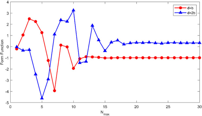
FIGURE 3. Convergence study of the T-matrix method for a pair of rigid spheres. The backscattering modulus $\left|f_{\infty }\right|$ of a pair of rigid spheres was calculated at end-on incidence (${\theta }_i=0°$) with the dimensionless frequency $kb=5$ versus $N_{\max }$ for a pair of rigid spheres with separation distances $2d=2b$ and $4b$, respectively.

The truncation factor $N_{\max }^{\prime }$ in this study is expressed as $N_{\max }^{\prime }=\mathrm{Int}\left(k\times \left(2d+r_0\right)\right)+5$. When the dimensionless frequency $kb=5$, the values of the truncation factor $N_{\max }^{\prime }$ are taken as 20 and 30 for separation distances of $d=b$ and $2b$, respectively. As shown in Figure 3, the form function modulus begins to converge, where $N_{\max }$ is greater than 14 and 26, respectively, and the relative convergence error could reach ${10}^{-5}\sim {10}^{-6}$. Therefore, the expression of the truncation factor $N_{\max }$ is verified to be correct and feasible. Furthermore, the convergence and accuracy of the T-matrix method for calculating the acoustic scattering of a pair of rigid spheroids are studied. Figure 4 shows the backscattering modulus $\left|f_{\infty }\right|$ of a pair of rigid spheroids with $b/a=4$ for the separation distance $2d=4r_0$ versus $N_{\max }$ with $kb=10$ under three incident cases (${\theta }_i=0°,45°,$ and $90°$). The results show that all the curves have good convergence and the solutions are stable and accurate. Similarly, the relative convergence error could reach ${10}^{-5}\sim {10}^{-6}$.

FIGURE 4

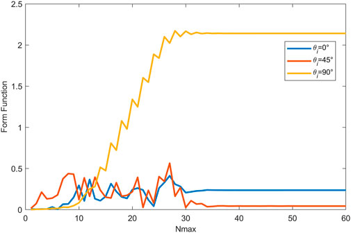
FIGURE 4. Convergence study of the T-matrix method for a pair of rigid spheroids with aspect ratio $b/a=4$ for the separation distance $2d=4r_0$. The backscattering modulus $\left|f_{\infty }\right|$ of a pair of rigid spheroids was calculated with the dimensionless frequency $kb=10$ versus $N_{\max }$ under three incident cases (${\theta }_i=0°,45°,$ and $90°$).

In the following, some numerical experiment results of the acoustic scattering of a pair of rigid spheres calculated by the present method are compared with Peterson’s works [19] and the analytical results. The comparison results are shown in Figure 5. The circles are values according to the data from Peterson’s works, while the solid lines are calculated by the present method. Panel (a) of Figure 5 displays the backscattering cross section of a pair of rigid spheres at the broadside incidence case (${\theta }_i={90}^{\circ },{\phi }_i=0^{\circ }$) for $kb=2$ versus the separation distance $2kd$. It can be seen from Panel (a) of the figure that the numerical results are in complete agreement with Peterson’s solutions. The scattering cross section is defined by

${\sigma }_N\left(r,{\theta }_s,{\phi }_s;{\theta }_i,{\phi }_i\right)=4\pi r^2\frac{{\left|{\mathrm{\Phi }}_s\right|}^2}{{\left|{\mathrm{\Phi }}_0\right|}^2}\frac{1}{\pi b^2}.(40)$

FIGURE 5

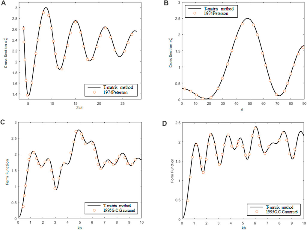
FIGURE 5. Accuracy study of the T-matrix method for a pair of rigid spheres. (A) Backscattering cross section of a pair of rigid spheres at broadside incidence (${\theta }_i=90°$) for $kb=2$ versus separation distance $2kd$. (B) Backscattering cross section of a pair of rigid spheres for $kb=2$ and $2kd=4.5$ versus the incidence angle ${\theta }_i$. (C) Backscattering form function $\left|f_{\infty }\right|$ of a pair of rigid spheres at broadside incidence (${\theta }_i=90°$) versus $kb$ for the separation distance $2d=2b$. (D) Backscattering form function $\left|f_{\infty }\right|$ of a pair of rigid spheres at broadside incidence (${\theta }_i=90°$) versus $kb$ for the separation distance $2d=2b$.

Panel (b) of Figure 5 displays the far-field backscattering cross section ${\sigma }_N$ versus the incidence angle ${\theta }_i$ of a pair of rigid spheroids for $kb=2$ and $2kd=4.5$. It is in complete agreement with the results in Figure 7 of Peterson’s works. It can be assured that the T-matrix method is sufficiently accurate in calculating the acoustic scattering of a pair of rigid spheres at arbitrary angular incidence. As shown in panels (c) and (d), the results of the backscattering form function $\left|f_{\infty }\right|$ of a pair of rigid spheres at the broadside incidence case calculated by the present method are exactly the same as those calculated by the analytical method [28] for separation distances $2d=2b$ and $4b$. It can be seen from the aforementioned comparison that the T-matrix method is effective in computing the acoustic scattering of a pair of rigid spheres and spheroids.

3.2 Far-field acoustic scattering properties of a pair of rigid spheres

In this part, the far-field scattering properties of a pair of rigid spheres under the plane wave at arbitrary incident angles are studied by the T-matrix method. Figure 6 displays the backscattering form function $\left|f_{\infty }\right|$ versus the dimensionless frequency $ka$ of a pair of rigid spheres with two values of the separation distance ($2d=2b$ and $4b$) under oblique (${\theta }_i=45°$) incidence and end-on (${\theta }_i=0°$) incidence, respectively. As shown in Panels (a) and (b), it can be seen that the form function $\left|f_{\infty }\right|$ (solid line) of a pair of spheres is below the values (dashed line) of twice the form function modulus of a single rigid sphere under plane wave oblique incidence. Furthermore, the backscattering form function curves oscillate faster as the separation distance increases at the oblique incidence case. This phenomenon is similar to the end-on incidence case (see Panels (c) and (d) of Figure 6), but the number of peaks in the backscattering form function curves under the oblique incidence case at the same separation distance is less than the end-on incidence case. In the end-on incidence case, the amplitude of the backscattering form function $\left|f_{\infty }\right|$ tends to be stable as $kb$ increases for the separation distance of $2d=4b$ (see Panel (d) of Figure 6). The reason for these oscillations in the backscattering form function curves is due to the interference between the specular reflection wave components and Franz wave components in the backscattering response wave [29, 30]. It can be seen that the oscillation period in the backscattering form function curves (solid line) of a pair of rigid spheres is not a constant compared to that (dashed line) of the single rigid sphere [31, 32]. The propagation mechanisms of the specular reflection and Franz wave in the backscattering response wave by a pair of rigid spheres are discussed in the following paragraph.

FIGURE 6

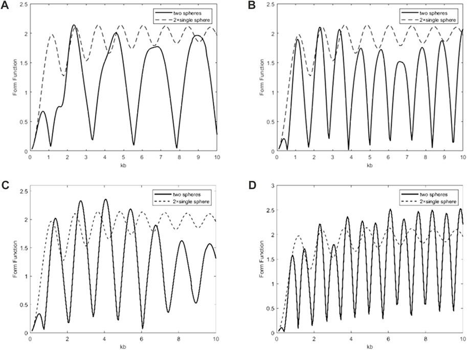
FIGURE 6. Backscattering form function $\left|f_{\infty }\right|$ (solid lines) of a pair of rigid spheres at oblique incidence (${\theta }_i=45°$) versus $kb$ for the separation distances (A) $2d=2b$ and (B) $2d=4b$. The backscattering form function $\left|f_{\infty }\right|$ of a pair of rigid spheres at end-on incidence (${\theta }_i=0°$) versus $kb$ for separation distances (C) $2d=2b$ and (D) $2d=4b$. The dashed lines represent twice the value of the backscattering form function $\left|f_{\infty }\right|$ of a single rigid sphere.

The path of backscattering waves by a pair of rigid spheres ensonified by the pulse wave from end-on incidence and oblique incidence, respectively, is shown in Panels (a) and (b) of Figure 7. $P_1$ and $P_3$ represent specular reflection waves, which propagate backwards immediately when the incident wave reaches the front of the first sphere and the second sphere, respectively. $P_2$ and $P_4$ represent the backward Franz waves, which diffracted around the shadowed surface of the obstacle, from the first sphere and second sphere, respectively. We define the moments of the arrival of backscattering response wave components $P_1$, $P_2$, $P_3$, and $P_4$ at the observation point as $t_1$, $t_2$, $t_3$, and $t_4$, respectively. The time intervals under end-on incidence can be predicted by the following equations:

$\left\{\begin{array}{l}{t}_2-t_1=\frac{\left(\overline{CD}+\mathit{DEF}+\overline{FG}\right)}{c},\\ t_3-t_1=2\times \left(\overline{CD}+\overline{DH}\right)/c,\\ t_4-t_3=\left(\overline{HI}+IJK+\overline{KL}\right)/c,\end{array}\right.(41)$

where $c$ denotes the velocity of the specular reflection wave. Likewise, the time intervals under the oblique incidence can be predicted as

$\left\{\begin{array}{l}{t}_2-t_1=\left(\overline{CD}+\mathit{DEF}+\overline{FG}\right)/c,\\ t_3-t_1=2\times \overline{MN}/c,\\ t_4-t_3=\frac{\left(\overline{HI}+IJK+\overline{KL}\right)}{c}.\end{array}\right.(42)$

FIGURE 7

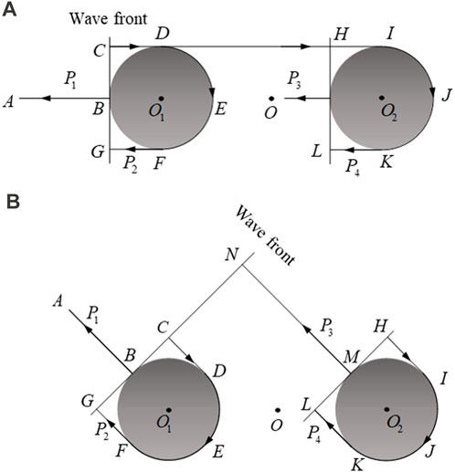
FIGURE 7. Propagation path of the backscattering waves by a pair of spheres at (A) end-on incidence and (B) oblique incidence.

The ideal fluid medium around the spheres is water. The velocity of the specular reflection wave is 1,510 m/s, and the scattering field point is located at (−30, 0). The time domain response results obtained by the inverse fast Fourier transform (IFFT) of the frequency domain response results [33] of a pair of rigid spheres at three incidence cases (${\theta }_i=0°,45°,\mathrm{a}\mathrm{n}\mathrm{d}90°$) of pulse waves for the separation distance $2d=4b=4m$ are shown in Figures 8A–C. Four obvious peaks can be obtained from Figures 8A, B. The specular reflection waves from the first sphere and second sphere lead to two peaks with the largest values. The two peaks with the smaller values are the Franz waves of the first sphere and second sphere, respectively. The values of Franz waves are smaller than those of specular reflection waves due to radiation damping when the Franz wave propagates in the shadowed area of the sphere. It can be seen that there are only two obvious peaks in Panel (c) of Figure 8 because the two spheres do not block each other in the direction of the pulse wave. In the case of broadside incidence (${\theta }_i=90°$), the specular reflection waves of two spheres reach the observing point at the same time, and subsequently, the Franz waves also reach the observing point at another identical time point. Furthermore, the time intervals corresponding to the peak-to-peak intervals for a pair of rigid spheres with three incidence cases (${\theta }_i=0°,45°,\mathrm{a}\mathrm{n}\mathrm{d}90°$) of the pulse wave for the separation distance $2d=4b=4m$ in Figure 8 are listed in Tables 1, 2, 3. The predicted results based on the geometric model are calculated from Eqs 41, 42. As can be seen from Tables 1, 2, 3, the results calculated by the T-matrix method are consistent with the predicted results from the geometric model.

FIGURE 8

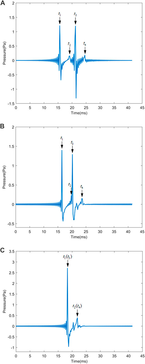
FIGURE 8. Backscattering response waves of a pair of rigid spheres in the time domain for the separation distance $2d=4b=4m$ under the pulse wave. (A) End-on incidence (${\theta }_i=0°$), (B) oblique incidence (${\theta }_i=45°$), and (C) broadside incidence (${\theta }_i=90°$).

TABLE 1

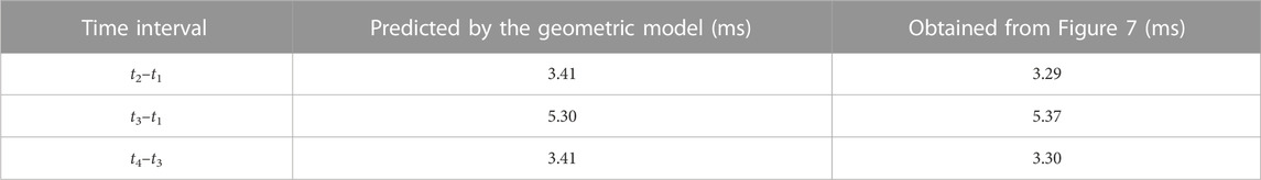
TABLE 1. Time intervals regarding the peak-to-peak intervals in Panel (a) of Figure 7.

TABLE 2

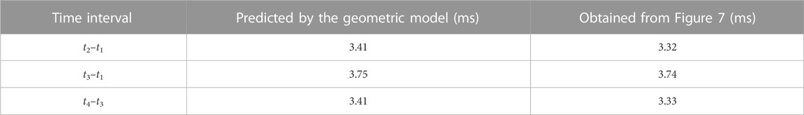
TABLE 2. Time intervals regarding the peak-to-peak intervals in Panel (b) of Figure 7.

TABLE 3

TABLE 3. Time intervals regarding the peak-to-peak intervals in Panel (c) of Figure 7.

In order to quantitatively study the scattering of a pair of rigid spheres, the bistatic 2D directivity plots of a pair of rigid spheres under three cases (${\theta }_i=0°,45°,\mathrm{a}\mathrm{n}\mathrm{d}90°$) of the plane waves for the dimensionless frequency $kb=2$ and separation distances $2d=2b$ and $4b$, respectively, are shown in Figures 9A–F. It can be found that the scattering form function $\left|f_{\infty }\right|$ (solid line) of a pair of spheres is mostly below the dashed line, which is twice the value of the form function of the single sphere. The maximum values of the scattering form function $\left|f_{\infty }\right|$ in the 2D far-field directivity plots are in the forward scattering direction under three cases. The 2D far-field directivity plots under the oblique incidence are asymmetric in Figures 9C, D because the obstacles are asymmetric along the wave axis in the oblique incidence case. It is clearly shown that the number of petals increased as the separation distance increases at the same incident angles.

FIGURE 9

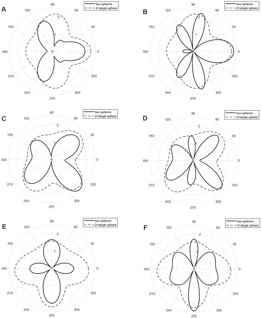
FIGURE 9. Bistatic 2D directivity pattern (solid line) of a pair of rigid spheres at end-on (${\theta }_i=0°$) incidence with $kb=2$ for separation distances (A) $2d=2b$ and (B) $2d=4b$. The bistatic 2D directivity pattern of a pair of rigid spheres at oblique (${\theta }_i=45°$) incidence with $kb=2$ for separation distances (C) $2d=2b$ and (D) $2d=4b$. The bistatic 2D directivity pattern of a pair of rigid spheres at broadside (${\theta }_i=90°$) incidence with $kb=2$ for separation distances (E) $2d=2b$ and (F) $2d=4b$. The dashed lines represent twice the value of the 2D directivity pattern of a single rigid sphere under three cases of incident angles (${\theta }_i=0°$, $45°$, and $90°$) for $kb=2$.

3.3 Far-field acoustic scattering properties of a pair of rigid spheroids

In this section, the far-field scattering properties of a pair of rigid spheroids under arbitrary incident angles of the plane wave are studied by the T-matrix method. The results of the backscattering form function $\left|f_{\infty }\right|$ (solid lines) of a pair of rigid prolate ($b/a=2$) spheroids at three incidence cases (${\theta }_i=0°,45°\mathrm{a}\mathrm{n}\mathrm{d}90°$) versus the non-dimensional frequency $k{r}_0$ ($r_0=\max \left(a,b\right)$) for the separation distance $2d=2r_0$ and $4r_0$, respectively, are shown in Figures 10A–F. The dashed lines represent twice the value of the backscattering form function $\left|f_{\infty }\right|$ of a single rigid sphere at broadside incidence. As shown in Figures 10A–D, the backscattering form function curves oscillate faster as the separation distance increases in the end-on incidence and oblique incidence cases. This phenomenon is consistent with the results of a pair of rigid sphere scattering in Section 3.2. Those oscillations in backscattering form function curves are caused by the interference between the specular reflection wave components and Franz wave components in the backscattering response wave. The peaks in the backscattering form function curves occur when the wave path difference $\Delta s$ between the Franz wave and specular reflection wave, which is related to the separation distance $2d$, is an integral multiple of the wavelength $\lambda$. The peak-to-peak interval $\Delta \left(k{r}_0\right)$ in the backscattering form function curves can be expressed as $\Delta \left(k{r}_0\right)=\frac{2\pi a}{\Delta s}$. Obviously, $\Delta \left(k{r}_0\right)$ decreases as the separation distance increases, making the backscattering form function curves oscillate faster. In the broadside incidence case, the solid line and dashed line overlap at low frequencies in Panel (e) of Figure 10, implying that there is no interaction between these two spheroids in this frequency band. As the separation distance grows, the solid line and dashed line still overlap at higher frequencies in Panel (f) of Figure 10. This is because the two spheroids do not block each other in the direction of the incident wave, and the interactions between these two spheroids decrease as the separation distance grows.

FIGURE 10

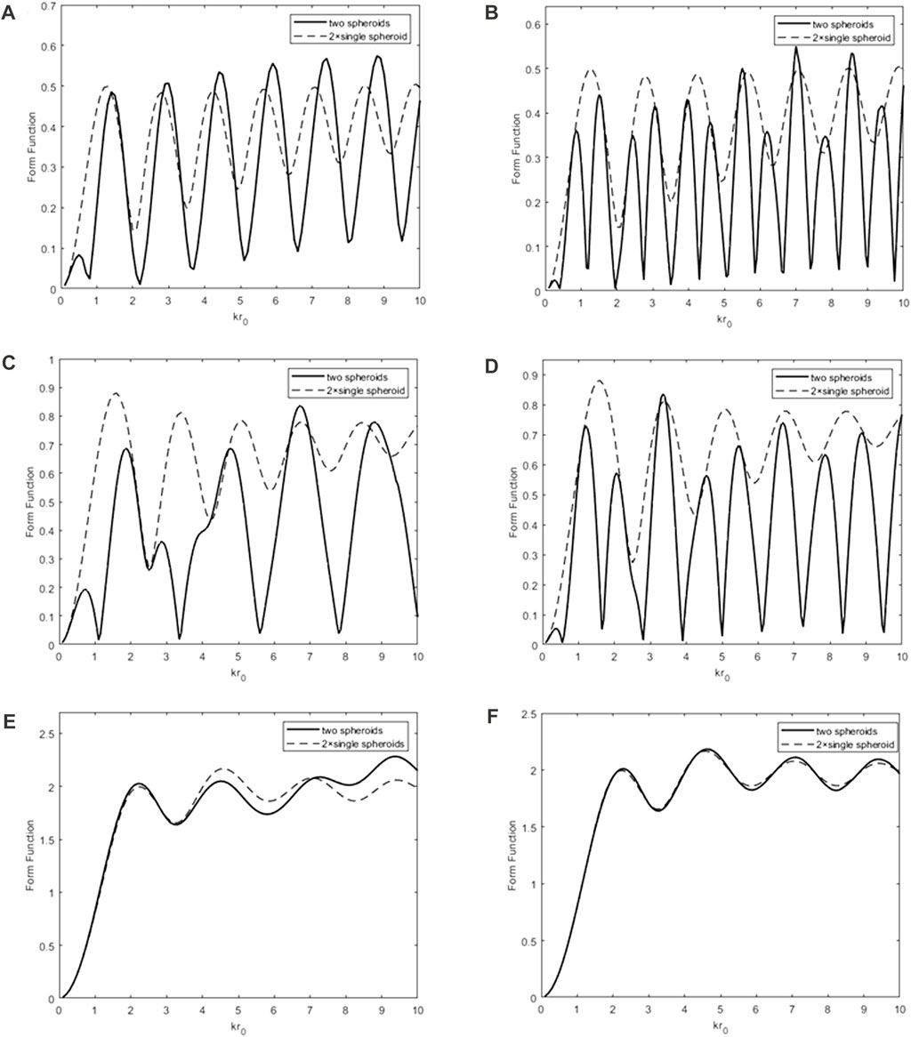
FIGURE 10. Backscattering form function $\left|f_{\infty }\right|$ (solid lines) of a pair of rigid prolate spheroids under end-on incidence (${\theta }_i=0°$) versus $k{r}_0$ ($r_0=\max \left(a,b\right)$) for separation distances (A) $2d=2r_0$ and (B) $2d=4r_0$. The backscattering form function $\left|f_{\infty }\right|$ (solid lines) of a pair of rigid prolate spheroids under oblique incidence (${\theta }_i=45°$) versus $kb$ for separation distances (C) $2d=2r_0$ and (D) $2d=4r_0$. The backscattering form function $\left|f_{\infty }\right|$ of a pair of rigid prolate spheroids under broadside incidence (${\theta }_i=90°$) versus $kb$ for separation distances (E) $2d=2b$ and (F) $2d=4b$. The dashed lines represent twice the value of the backscattering form function $\left|f_{\infty }\right|$ of a single rigid prolate spheroid under three incident cases (${\theta }_i=0°$, $45°$, and $90°$).

Figure 11 displays the backscattering form function $\left|f_{\infty }\right|$ of a pair of rigid spheroids with different aspect ratios ($b/a=1/2$, $1$, $2$, and $4$) versus $k{r}_0$ ($r_0=\max \left(a,b\right)$) for the separation distance $2d=4r_0$ at three incidence cases (${\theta }_i=0°,45°,\mathrm{a}\mathrm{n}\mathrm{d}90°$). As shown in Figure 11A, the values of the backscattering form function $\left|f_{\infty }\right|$ of a pair of rigid spheroids in the end-on incidence case decrease as the aspect ratios grow. This is because the backscattering response wave of a pair of rigid spheroids under plane wave end-on incidence is mainly composed of the specular reflection wave at the front point of the spheroids, and the intensity of the specular reflection wave increases as the radius of curvature at the front point of the spheroids increases [34]. It can be seen from Figure 11 that the number of peaks in the backscattering form function curves for a pair of rigid prolate ($b>a$) spheroids decreases with the increase in the incidence angle. In order to quantitatively study the scattering of a pair of rigid spheroids under the plane wave, the bistatic 2D directivity plots for a pair of rigid spheroids with different aspect ratios ($b/a=1/2$, $1$, $2$, and $4$) at three incidence cases (${\theta }_i=0°,45°,\mathrm{a}\mathrm{n}\mathrm{d}90°$) of the plane waves for the non-dimensional frequency $kb=2$ and separation distances $2d=2r_0$ and $4r_0$, respectively, are shown in Figures 12A–F. The zoomed-in plots regarding the results of the 2D directivity diagrams of a pair of rigid prolate spheroids ($b/a=4$) are also given in these panels. It is clearly seen that the number of petals in the 2D directivity plots is mainly influenced by the separation distance, and the number of petals increased as the separation distance increased. The 2D directivity plots are asymmetric in Figures 12C, D because the scatterers are asymmetric along the wave axis in the oblique incidence case, which is different from the end-on incidence and broadside incidence case. In the end-on incidence case (see Figures 12A, B), the 2D directivity plots of a pair of rigid spheroids change from the forward scattering dominant to the sideward scattering dominant, with the increase in the aspect ratio. The maximum values in the 2D far-field directivity plots of a pair of rigid spheroids decrease as the aspect ratio increases in the end-on incidence and oblique incidence cases. In the broadside incidence case (Figures 12E, F), the 2D directivity plots of a pair of oblate spheroids and prolate spheroids are sideward scattering dominant and backward scattering dominant, respectively. It can be found that the 2D far-field directivity plots of a pair of rigid prolate spheroids with different aspect ratios at the same incident angle and separation distance are very similar, and the values of the scattering form function $\left|f_{\infty }\right|$ decreases as the aspect ratio increases.

FIGURE 11

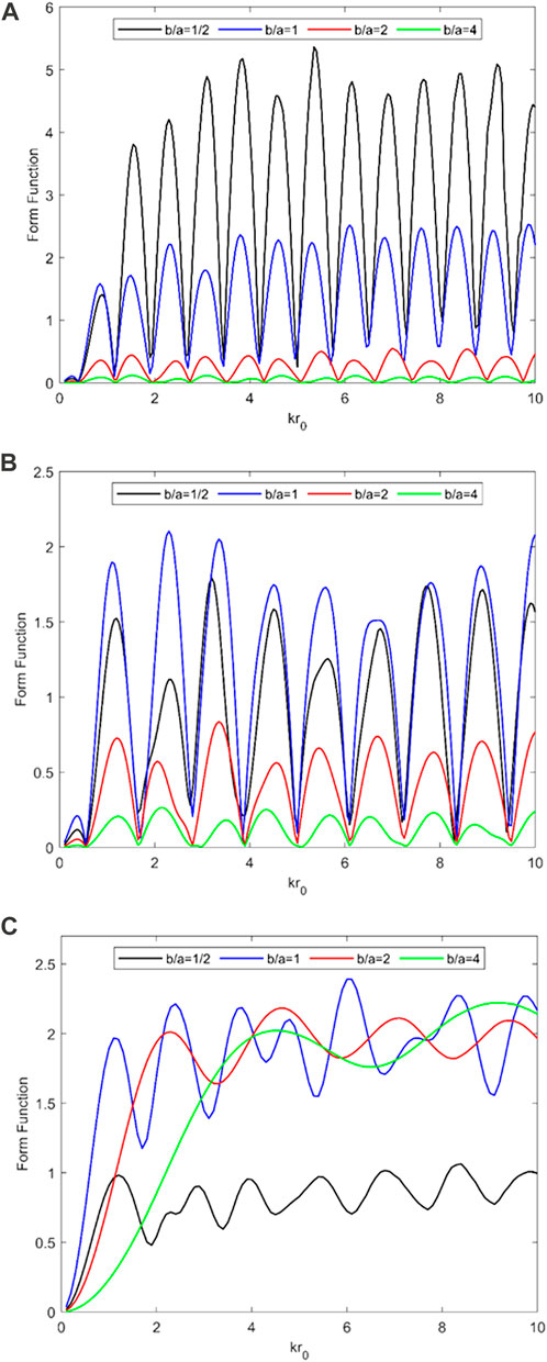
FIGURE 11. Backscattering form function $\left|f_{\infty }\right|$ of a pair of rigid spheroids with different aspect ratios ($b/a=1/2$, $1$, $2$, and $4$) versus $k{r}_0$ for the separation distance $2d=4r_0$ under the plane wave. (A) End-on incidence (${\theta }_i=0°$), (B) oblique incidence (${\theta }_i=45°$), and (C) broadside incidence (${\theta }_i=90°$).

FIGURE 12

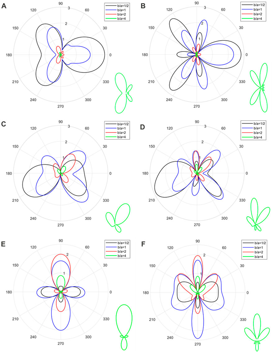
FIGURE 12. Bistatic 2D directivity pattern of a pair of rigid spheroids with different aspect ratios ($b/a=1/2$, $1$, $2$, and $4$) at end-on incidence (${\theta }_i=0°$) with $k{r}_0=2$ for separation distances. (A) $2d=2r_0$ and (B) $2d=4r_0$. The bistatic 2D directivity pattern of a pair of rigid spheroids with different aspect ratios ($b/a=1/2$, $1$, $2$, and $4$) at oblique incidence (${\theta }_i=45°$) with $k{r}_0=2$ for separation distances (C) $2d=2r_0$ and (D) $2d=4r_0$. The bistatic 2D directivity pattern of a pair of rigid spheroids with different aspect ratios ($b/a=1/2$, $1$, $2$, and $4$) at broadside incidence (${\theta }_i=90°$) with $k{r}_0=2$ for separation distances (E) $2d=2r_0$ and (F) $2d=4r_0$.

4 Conclusion

In this work, the T-matrix method combined with the addition theorems of spherical basis functions is applied to semi-analytically compute the far-field acoustic scattering of a pair of rigid spheroids under the plane wave at an arbitrary incidence angle. It is verified that the T-matrix method can accurately solve the far-field acoustic scattering problem of a pair of rigid spheres with different separation distances under the plane wave of any angle. In addition, some numerical experiments on a pair of rigid (oblate or prolate) spheroids are carried out by the T-matrix method with the following conclusions:

1) The acoustic scattering by a pair of rigid spheroids is more complicated than that of a single rigid spheroid, and the values of the scattering form function of a pair of rigid spheroids are not equal to twice the far-field scattering form function modulus of a single rigid spheroid.

2) The peak-to-peak interval of the backscattering response curve obtained by the IFFT in the time domain is consistent with the geometric prediction results, which makes it possible to estimate the geometrical dimension and separation distance of multiple scatterers from the scattering response wave.

3) The parameters affecting the far-field scattering form function modulus of a pair of rigid spheroids are aspect ratio $b/a$, separation distance $2d$, dimensionless frequency $k{r}_0$ ($r_0=\max \left(a,b\right)$), and incident angle ${\theta }_i$.

Data availability statement

The original contributions presented in the study are included in the article/Supplementary Material; further inquiries can be directed to the corresponding author.

Author contributions

WL conceptualized this investigation. YY performed the formal analysis and validation. YY performed the data analysis with advice from QG, YZ, YC, and WL. YY wrote the manuscript. All authors contributed to the article and approved the submitted version.

Conflict of interest

The authors declare that the research was conducted in the absence of any commercial or financial relationships that could be construed as a potential conflict of interest.

Publisher’s note

All claims expressed in this article are solely those of the authors and do not necessarily represent those of their affiliated organizations, or those of the publisher, the editors, and the reviewers. Any product that may be evaluated in this article, or claim that may be made by its manufacturer, is not guaranteed or endorsed by the publisher.

References

1. Seybert AF, Rengarajan TK. The use of CHIEF to obtain unique solutions for acoustic radiation using boundary integral equations. The J Acoust Soc America (1987) 81(5):1299–306. doi:10.1121/1.2024508

CrossRef Full Text | Google Scholar

2. Hunt JT, Knittel MR, Barach D. Finite element approach to acoustic radiation from elastic structures. The J Acoust Soc America (1974) 55(2):269–80. doi:10.1121/1.1914498

CrossRef Full Text | Google Scholar

3. Seybert AF, Soenarko B, Rizzo FJ, Shippy DJ. An advanced computational method for radiation and scattering of acoustic waves in three dimensions. J Acoust Soc America (1985) 77(2):362–8. doi:10.1121/1.391908

CrossRef Full Text | Google Scholar

4. Chai YB, Li W, Gong ZX, Li TY. Hybrid smoothed finite element method for two-dimensional underwater acoustic scattering problems. Ocean Eng (2016) 116:129–41. doi:10.1016/j.oceaneng.2016.02.034

CrossRef Full Text | Google Scholar

5. Li W, Chai YB, Lei M, Li TY. Numerical investigation of the edge-based gradient smoothing technique for exterior Helmholtz equation in two dimensions. Comput Structures (2017) 182:149–64. doi:10.1016/j.compstruc.2016.12.004

CrossRef Full Text | Google Scholar

6. You X, Gui Q, Zhang Q, Chai Y, Li W. Meshfree simulations of acoustic problems by a radial point interpolation method. Ocean Eng (2020) 218:108202. doi:10.1016/j.oceaneng.2020.108202

CrossRef Full Text | Google Scholar

7. Gui Q, Zhang G, Chai Y, Li W. A finite element method with cover functions for underwater acoustic propagation problems. Ocean Eng (2022) 243:110174. doi:10.1016/j.oceaneng.2021.110174

CrossRef Full Text | Google Scholar

8. Rayleigh JWSB. The theory of sound. London: Macmillan &Company (1896).

Google Scholar

9. Faran JJ. Sound scattering by solid cylinders and spheres. The J Acoust Soc America (1951) 23(4):405–18. doi:10.1121/1.1906780

CrossRef Full Text | Google Scholar

10. Morse PMC, Ingard KU. Theoretical acoustics. New Jersey: Princeton university press (1986).

Google Scholar

11. Záviška F. Über die Beugung elektromagnetischer Wellen an parallelen, unendlich langen Kreiszylindern. Annalen der physik (1913) 4(40):1023–56. doi:10.1002/andp.19133450511

CrossRef Full Text | Google Scholar

12. Williams KL, Marston PL. Backscattering from an elastic sphere: Sommerfeld–Watson transformation and experimental confirmation. J Acoust Soc America (1985) 78(3):1093–102. doi:10.1121/1.393028

CrossRef Full Text | Google Scholar

13. Eyges L. Some nonseparable boundary value problems and the many-body problem. Ann Phys (1957) 2(2):101–28. doi:10.1016/0003-4916(57)90037-4

CrossRef Full Text | Google Scholar

14. Sack RA. Three-dimensional addition theorem for arbitrary functions involving expansions in spherical harmonics. J Math Phys (1964) 5:252–9. doi:10.1063/1.1704115

CrossRef Full Text | Google Scholar

15. Gabrielli P, Mercier-Finidori M. Acoustic scattering by two spheres: Multiple scattering and symmetry considerations. J Sound Vibration (2001) 241(3):423–39. doi:10.1006/jsvi.2000.3309

CrossRef Full Text | Google Scholar

16. Gaspard P, Rice SA. Exact quantization of the scattering from a classically chaotic repellor. J Chem Phys (1989) 90(4):2255–62. doi:10.1063/1.456019

CrossRef Full Text | Google Scholar

17. Waterman PC. Matrix formulation of electromagnetic scattering. Proceeding of the IEEE (1965) 53(8):805–12. doi:10.1109/PROC.1965.4058

CrossRef Full Text | Google Scholar

18. Waterman PC. New formulation of acoustic scattering. J Acoust Soc America (1969) 45(6):1417–29. doi:10.1121/1.1911619

CrossRef Full Text | Google Scholar

19. Peterson B, Ström S. Matrix formulation of acoustic scattering from an arbitrary number of scatterers. J Acoust Soc America (1975) 56:771–80. doi:10.1121/1.1903325

CrossRef Full Text | Google Scholar

20. Mishchenko MI. Electromagnetic scattering by particles and particle groups: An introduction. New York: Cambridge University press (2014).

Google Scholar

21. Mishchenko MI, Hovenier JW, Tracis LD. Light scattering by nonspherical particles: Theory, measurements, and applications. Academic Press (1986).

Google Scholar

22. Danos M, Maximon LC. Multipole matrix elements of the translation operator. J Math Phys (1965) 6(5):766–78. doi:10.1063/1.1704333

CrossRef Full Text | Google Scholar

23. Gonis A, Butler WH. Multiple scattering in solids. New York: Springer (2000).

Google Scholar

24. Edmonds AR. Angular momentum in quantum mechanics. Princeton, NJ: Princeton University Press (1974).

Google Scholar

25. Neubauer WG, Vogt RH, Dragonette LR. Acoustic reflection from elastic spheres. I. Steady-state signals. J Acoust Soc America (1974) 55:1123–9. doi:10.1121/1.1914676

CrossRef Full Text | Google Scholar

26. Dragonette LR, Vogt RH, Flax L, Neubauer WG. Acoustic reflection from elastic spheres and rigid spheres and spheroids. II. Transient analysis. J Acoust Soc America (1974) 55:1130–7. doi:10.1121/1.1914677

CrossRef Full Text | Google Scholar

27. Li W, Chai YB, Gong ZX, Marston PL. Analysis of forward scattering of an acoustical zeroth-order Bessel beam from rigid complicated (aspherical) structures. J Quantitative Spectrosc Radiative Transfer (2017) 200:146–62. doi:10.1016/j.jqsrt.2017.06.002

CrossRef Full Text | Google Scholar

28. Gaunaurd GC, Huang H, Strifors HC. Acoustic scattering by a pair of spheres. J Acoust Soc America (1995) 98:495–507. doi:10.1121/1.414447

CrossRef Full Text | Google Scholar

29. Pillai TAK, Varadan VV, Varadan VK. Sound scattering by rigid and elastic infinite elliptical cylinders in water. J Acoust Soc America (1982) 72:1032–7. doi:10.1121/1.388234

CrossRef Full Text | Google Scholar

30. Eastland GC, Marston PL. Enhanced backscattering in water by partially exposed cylinders at free surfaces associated with an acoustic Franz wave. J Acoust Soc America (2014) 135:2489–92. doi:10.1121/1.4870240

PubMed Abstract | CrossRef Full Text | Google Scholar

31. Gong ZX, Li W, Mitri FG, Chai YB, Zhao Y. Arbitrary scattering of an acoustical Bessel beam by a rigid spheroid with large aspect-ratio. J Sound Vibration (2016) 383:233–47. doi:10.1016/j.jsv.2016.08.003

CrossRef Full Text | Google Scholar

32. Gong ZX, Li W, Chai YB, Zhao Y, Mitri FG. T-matrix method for acoustical Bessel beam scattering from a rigid finite cylinder with spheroidal endcaps. Ocean Eng (2017) 129:507–19. doi:10.1016/j.oceaneng.2016.10.043

CrossRef Full Text | Google Scholar

33. Li W, Liu GR. Estimation of radius and thickness of a thin spherical shell in water using the midfrequency enhancement of a short tone burst response. J Acoust Soc America (2005) 118:2147–53. doi:10.1121/1.2040027

CrossRef Full Text | Google Scholar

34. Tang WL. Highlight model of echoes from sonar targets. Chin J Acoust (1994) 13:131–40. doi:10.15949/j.cnki.0217-9776.1994.02.004

CrossRef Full Text | Google Scholar