Dynamic analysis and optimal control of a stochastic information spreading model considering super-spreader and implicit exposer with random parametric perturbations

Environmental factors in social systems affect information spreading at all times. This paper proposes a stochastic S2EIR model that considers the presence of super-spreaders and implicit exposers in information spreading, as well as the stochastic perturbation of model parameters. The existence of a global positive solution using the $It{\widehat{o}}^{\prime }s$ formula is then demonstrated. Sufficient conditions for information disappearance and smooth distribution of information are calculated by using the Borel–Cantelli lemma and the strong law of large numbers. Furthermore, the optimal control strategy for the stochastic model is proposed using the Hamiltonian function. The results of the theoretical analysis are supported by numerical simulations and compared to the parameter variations of the deterministic model. The results of this study indicate that white noise facilitates the spread of information. The intensity of perturbation is proportional to the fluctuation of information spreading. Controlling random parameters can effectively facilitate the spread of information. For positive information, the randomness and complexity of the social system should be utilized to increase the spread of information. In contrast, for negative information, randomness in the social system should be suppressed to the greatest extent possible to limit information dissemination.

1 Introduction

Information is essential to the development of human society and is the primary means by which humans can comprehend society and improve their cognition. In general, the effects of various types of information on society vary. Information that is beneficial to social development, such as knowledge, innovation, and affinity, must be disseminated [1]; [2]; [3]; [4], while information that is harmful to social development, such as rumors and computer viruses, must be contained [5]; [6]; [7]. Therefore, it is valuable to investigate the characteristics and mechanisms of information dissemination.

Information dissemination is similar to the spread of infectious diseases. Daley and Kendall [8] first applied the classical infectious disease model to the spread of rumors in order to study the spread of harmful information, and they proposed the classical rumor spread DK model. The SI model [9], the SIS model [10], the SIR model [11], and other infectious disease models were then used as a research foundation to propose the SEIR model [12], the SPNR model [13], the ILSR model [14], etc.

The aforementioned models typically regard environmental factors as deterministic factors and do not account for them. However, there are many uncertain environmental factors in the real social environment. Random factors, such as government regulation of the media, sudden mass events, and outbreaks of epidemics or geological disasters, can interfere with the dissemination of information [15]. Therefore, researchers are beginning to consider the impact of uncertain environmental factors on the spread of information.

In recent years, extensive studies on stochastic factors in the field of virus propagation have been proposed. Shang [16] developed a low-dimensional system of nonlinear ordinary differential equations to model the mixed susceptible–infected (–recovered) SI(R) epidemics on a random network with general degree distributions. Zhang and Li [17] developed the stochastic SEIR model with migration and human awareness in complex networks and compared the distance between stochastic and deterministic systems at points of local disease equilibrium. Liu and Jiang [18] developed the stochastic SEIR model with asymptomatic infected individuals and calculated the specific form of the probability density near the quasi-endemic equilibrium of the stochastic system. Hussain et al. [19] proposed the stochastic SIRV model with general nonlinear incidence and vaccination and argued that stochastic fluctuations could limit the spread of disease. Wang et al. [20] designed the stochastic SICA model with standard incidence rates, provided sufficient conditions for HIV extinction and persistence, and discovered that increasing the intensity of stochastic perturbations could control the virus’s spread. Bobryk [21] believed that the spread rate in the SIR model must be positive, so he incorporated telegraphic noise, trichotomous noise, and bounded noise into the stochastic model and then discussed the effect of the stochastic perturbation on the stability behavior of disease-free equilibrium points. Kiouach and Sabbar [22] used Gaussian white noise and Lévy jumps to represent, respectively, parametric perturbations in stochastic models, and they calculated the disease’s mean persistence, ergodicity, and extinction. In addition, the application of infectious disease models with stochastic parameter perturbations to the novel coronavirus has been a hot topic over the past few years [23]; [24]; [25].

In the field of information spread, researchers have focused on the impact of stochastic factors on models of rumor spread. Cheng et al. [26] argued that individual activities play a significant role in rumor spread and that individual activities are affected by many uncertainties. As a result, they constructed the I_aI_dS_aS_dR_aR_d model and analyzed the dynamical behavior of the stochastic model based on this argument. Zhang and Zhu [27] concluded that the spread rate among individuals in rumor spread models is usually disturbed by random factors, and increasing the noise intensity can effectively control the spread of rumors. Tong et al. [28] constructed a stochastic rumor spread model with media coverage and age structure based on a deterministic model and confirmed the existence of a global positive solution to the model and the necessary conditions for rumor disappearance and smooth distribution. Zhou et al. [29] argued that information intervention influences rumor spread; consequently, they developed a stochastic SIRZ rumor spread model considering the information intervention mechanism and proposed an optimal control strategy for rumor control. Yue and Huo [30] developed a stochastic SICR rumor spreading model that accounted for media coverage and science education; the study’s results demonstrated that media coverage could inhibit rumor spread. Jain et al. [31] proposed the S₁S₂I model with expert interaction on a homogeneous network and discovered that noise perturbation caused persistent rumor spread. Huo and Dong [32] developed a stochastic ISR model with white noise media coverage, and the results of their study demonstrated that media coverage was inversely proportional to rumor spread. In addition, Mena et al. [33] analyzed the spread characteristics by developing an optimal control model based on the analysis of extinction and persistence of uncertain spread models.

The aforementioned scholars have conducted numerous studies on the influence of random factors on disease spread and rumor spread. In contrast, not all information is harmful to society in the real world, and positive information must be disseminated. Some beneficial information to society may be disseminated by individuals with authority, also known as super-spreaders. Then, it is more likely that the exposers who are in contact with the super-spreaders will comprehend and continue to spread the information. Conversely, the exposers who are not in contact with the super-spreaders are less likely to do so. The former is referred to as explicit spreaders, whereas the latter is referred to as implicit spreaders. This paper develops a stochastic S2EIR model that takes super-spreaders and exposers into account. Afterward, the existence of global positive solutions is demonstrated, suitable parameters are selected as control variables after calculating sufficient conditions for information disappearance and smooth information distribution, and the validity of the proposed theorem is validated through numerical simulation. Different from previous studies, this article considers that individuals with strong influence have played a significant role in promoting information spreading while also considering that some individuals are unwilling to spread information even if they are aware of it. Therefore, the common phenomena of “super-spreader” and “asymptomatic infection” in virus spreading are applied to the information spreading model. In addition, for each individual, the contact rate with information spreaders and the spread rate of being an information spreader may be affected by random perturbations in the environment. So, it is more practical to add random factors to the information spreading model. Meanwhile, the optimal control strategy containing random parameters of this paper is based on the optimal values calculated by the control variables.

The remainder of the paper is organized as follows. In Section 2, the stochastic S2EIR model taking super-spreaders and exposers into account is constructed. Section 3 proves the existence of a global positive solution. In Section 4, sufficient conditions for the disappearance of information are outlined. Section 5 provides sufficient conditions for stationary information distribution. The existence of optimal control and the optimal control strategy are discussed in Section 6. In Section 7, numerical simulation is used to analyze the impact of stochastic disturbance intensity on information spread and the effect of the control strategy. In the last section, conclusions are provided.

2 The model

This paper examines an open virtual community whose population size fluctuates over time t. The total population size can be represented by N(t), where all populations can be divided into five categories: 1) the receptive population S(t) who do not have access to information but are receptive to it; 2) the explicitly exposed population E₁(t) that has contact with the super-spreaders; 3) the implicitly exposed population E₂(t) that does not have contact with the super-spreaders; 4) the spread-information population I(t); and 5) the non-receptive population R(t) that is no longer interested in the information.

The model flow diagram is presented in Figure 1.

FIGURE 1

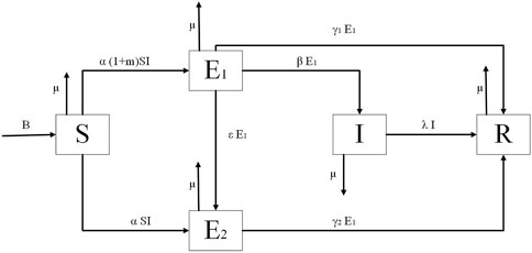
FIGURE 1. Flow diagram of the model.

In the model of this paper, the implicit exposers are rather special. People who are not influenced by the information’s super-spreaders typically do not easily comprehend the information’s content since it is spread by super-spreaders. Then, these people demonstrate a lack of interest in the information. Therefore, despite being exposed to the information, these individuals choose not to spread it.

The parameters in the S2EIR model can be interpreted as follows:

1) The number of individuals in a social system fluctuates over time. Therefore, in this paper, the author defines B as the number of individuals moving into the social system and defines μ as the emigration rate that is out of the social system due to force majeure factors.

2) When information begins to spread through the social system, the receptive population will contact the spreaders with a probability of α. The proportion of super-spreaders is defined as m. Since super-spreaders will speed up the information spread, the spread rate of explicit exposers is defined as α(1 + m), and the spread rate of implicit exposers is represented by α.

3) After the exposers make sense of the information, a portion of the explicit exposers who are interested in the information becomes the information spreaders with a probability of β. Additionally, the explicit exposers who are not interested in the information become implicit exposers with a probability of ϵ.

4) Due to the different degrees of information acceptance among the exposers, the two types of exposers become the non-receptive population with probabilities of γ₁ and γ₂. Information is generally time-sensitive, and some spreaders lose interest in the information after a period of time. As a result, they become the non-receptive population with a probability of λ.

In addition, the uncertain factors in social systems are commonly referred to as environmental noise. It is not scientific to study the spread of information while ignoring random environmental noise fluctuations. Incorporating environmental noise into deterministic models is more representative of how information spreads in real society. The random factors added to the spread models mainly include three classical approaches: 1) Introducing Gaussian white noise into deterministic parameter perturbation models [34]. 2) Random perturbation encompassing the positive endemic equilibrium of deterministic models [35]. 3) Alternating between regimes based on the probability of Markov chains [36]. Since random perturbations in the environment may affect the contact rate of each individual with the information spreader and the spread rate of becoming an information spreader, this paper uses Gaussian white noise to generate random perturbations of α and β, and the parameters of random perturbation are expressed as follows:

$\alpha \to \alpha +{\sigma }_1{\dot{W}}_1\left(t\right),\beta \to \beta +{\sigma }_2{\dot{W}}_2\left(t\right).(1)$

Here, W_i(i = 1, 2) are independent standard Brownian motions and ${\sigma }_i^2>0(i=\mathrm{1,2})$ represent the intensities of W_i(i = 1, 2), respectively. In this paper, W₁ and W₂ represent the relationship without mutual influence between α and β, respectively. In other words, in real scenarios, the conversion rate of information disseminators may be influenced by individual understanding and information acceptability, but it is not affected by the natural contact rate, and there is a state of mutual independence between the two.

The stochastic perturbation parameters are introduced into the deterministic model to construct a stochastic S2EIR model driven by Gaussian white noise, and the stochastic model can be represented as follows:

$\begin{array}{c}\hfill \left\{\begin{array}{c}dS\left(t\right)=\left[B-\alpha \left(1+m\right)SI-\alpha SI-\mu S\right]dt-{\sigma }_1\left(1+m\right)SId{W}_1\left(t\right)\hfill \\ -{\sigma }_{1}SId{W}_1\left(t\right),\hfill \\ d{E}_1\left(t\right)=\left[\alpha \left(1+m\right)SI-\beta E_1-{\gamma }_1{E}_1-\epsilon E_1-\mu E_1\right]dt\hfill \\ +{\sigma }_1\left(1+m\right)SId{W}_1\left(t\right)-{\sigma }_2{E}_{1}d{W}_2\left(t\right),\hfill \\ d{E}_2\left(t\right)=\left(\alpha SI+\epsilon E_1-{\gamma }_2{E}_2-\mu E_2\right)dt+{\sigma }_{1}SId{W}_1\left(t\right),\hfill \\ dI\left(t\right)=\left(\beta E_1-\lambda I-\mu I\right)dt+{\sigma }_2{E}_{1}d{W}_2\left(t\right).\hfill \end{array}\right.\end{array}(2)$

3 Existence of the global and positive solution

In the rest of this paper, let $(\mathrm{\Omega },\mathcal{F},{\{{\mathcal{F}}_t\}}_{t\ge 0},P)$ be a complete probability space with a filtration ${\{{\mathcal{F}}_t\}}_{t\ge 0}$ satisfying the usual conditions. In addition, while ${\mathcal{F}}_0$ contains all P − null sets, it is increasing and right continuous [37]. It also can be denoted as follows:

${\mathbb{R}}_{+}^4=\left\{\left(x_1,x_2,x_3,x_4\right)|x_i>0,i=\mathrm{1,2,3,4}\right\}.(3)$

The existence of the global solution is the basis of analyzing the dynamic behavior of the stochastic system (Eq. 2). At the same time, according to the actual situation, a positive value is required for the dynamic model of information transmission. The stochastic system (Eq. 2) can be proved as global and positive by Theorem 3.1.

Theorem 3.1. The existence of a unique positive solution $(S(t),E_1(t),E_2(t),I(t))\in {\mathbb{R}}_{+}^4$ of the stochastic system (Eq. 2) is satisfied by any given initial value $(S(t),E_1(t),E_2(t),I(t))\in {\mathbb{R}}_{+}^4$. The probability of the solution is 1 and remains in ${\mathbb{R}}_{+}^4$.

Proof. The existence of a unique local positive solution $(S(t),E_1(t),E_2(t),I(t))\in {\mathbb{R}}_{+}^4$ of the stochastic system (Eq. 2) on t ∈ [0, τ_e), which is based on the coefficients of the deterministic system, is locally Lipschitz continuous of any given initial value $(S(0),E_1(0),E_2(0),I(0))\in {\mathbb{R}}_{+}^4$. τ_e is the explosion time [38]. It is required to have τ_e = ∞ a.s. to show this solution globally. The stopping time τ⁺ can be defined by

${\tau }^{+}=\inf \left\{t\in \left[0,{\tau }_e\right):S\left(t\right)\ge 0or{\mathrm{E}}_1\left(t\right)\ge 0or{\mathrm{E}}_2\left(t\right)\ge 0orI\left(t\right)\ge 0\right\}.(4)$

Let set inf ∅ = ∞ (∅ denotes the empty set). It is easy to get τ⁺ ≤ τ_e. So, if τ⁺ = ∞ a.s. is proved, then τ_e = ∞ and $(S(t),E_1(t),E_2(t),I(t))\in {\mathbb{R}}_{+}^4$ a.s. for all t ≥ 0. We assume that τ⁺ < ∞; then, T > 0 is existence such that P(τ⁺ < T) > 0. We define ${\mathcal{C}}^2$ function V: ${\mathbb{R}}_{+}^4\to {\mathbb{R}}_{+}^4$ by V(X) = InSE₁E₂I. Using the $It{\widehat{o}}^{\prime }s$ formula, we calculate the differential of V along the solution trajectories of the stochastic system (2). For ω ∈ (τ⁺ < T) and for all t ∈ [0, τ_e), we get

$\begin{array}{c}\hfill \begin{array}{c}dV\left(X\left(t\right)\right)=\left[\frac{B}{S}-\alpha \left(1+m\right)I-\alpha I-\mu -\frac{1}{2}{\sigma }_1^2{\left(1+m\right)}^2{I}^2-\frac{1}{2}{\sigma }_1^2{I}^2\right]dt\hfill \\ +\left[\frac{\alpha \left(1+m\right)SI}{E_1}-\left(\beta +{\gamma }_1+\epsilon +\mu \right)-\frac{1}{2}{\sigma }_1^2\frac{{\left(1+m\right)}^2{S}^2{I}^2}{E_1^2}-\frac{1}{2}{\sigma }_2^2\right]dt\hfill \\ +\left[\frac{\alpha SI}{E_2}+\frac{\epsilon E_1}{E_2}-\left({\gamma }_2+\mu \right)-\frac{1}{2}{\sigma }_1^2\frac{S^2{I}^2}{E_2^2}\right]dt+\left[\frac{\beta E_1}{I}-\left(\lambda +\mu \right)\right.\hfill \\ \left.-\frac{1}{2}{\sigma }_2^2\frac{E_1^2}{I^2}\right]dt-{\sigma }_1\left(1+m\right)Id{W}_1-{\sigma }_{1}Id{W}_1+\frac{{\sigma }_1\left(1+m\right)SI}{E_1}d{W}_1\hfill \\ -{\sigma }_{2}d{W}_2+\frac{{\sigma }_{1}SI}{E_2}d{W}_1+\frac{{\sigma }_2{E}_1}{I}d{W}_2.\hfill \end{array}\end{array}(5)$

Positivity of X(t) implies that

$\begin{array}{c}\hfill \begin{array}{c}dV\left(X\left(t\right)\right)\ge L\left(S,E_1,E_2,I\right)dt-{\sigma }_1\left[\left(1+m\right)I+I-\frac{\left(1+m\right)SI}{E_1}-\frac{SI}{E_2}\right]d{W}_1\hfill \\ -{\sigma }_2\left(1-\frac{E_1}{I}\right)d{W}_2,\hfill \end{array}\end{array}(6)$

where

$\begin{array}{c}\hfill \begin{array}{c}L\left(S,E_1,E_2,I\right)=-\mu -\left(\beta +{\gamma }_1+\epsilon +\mu \right)-\left({\gamma }_2+\mu \right)-\left(\lambda +\mu \right)-\frac{1}{2}{\sigma }_1^2{\left(1+m\right)}^2{I}^2\hfill \\ -\frac{1}{2}{\sigma }_1^2{I}^2-\frac{1}{2}{\sigma }_1^2\frac{{\left(1+m\right)}^2{S}^2{I}^2}{E_2^2}-\frac{1}{2}{\sigma }_1^2\frac{S^2{I}^2}{E_2^2}-\frac{1}{2}{\sigma }_2^2-\frac{1}{2}{\sigma }_2^2\frac{E_1^2}{I^2}.\hfill \end{array}\end{array}(7)$

So, we have

$\begin{array}{c}\hfill \begin{array}{c}V\left(X\left(t\right)\right)\ge V\left(X_0\right)+{\int }_0^{t}L\left(S\left(u\right),E_1\left(u\right),E_2\left(u\right),I\left(u\right)\right)du\hfill \\ -{\int }_0^t{\sigma }_1\left[I\left(u\right)-\frac{\left(1+m\right)S\left(u\right)I\left(u\right)}{E_1\left(u\right)}-\frac{S\left(u\right)I\left(u\right)}{E_2\left(u\right)}\right]d{W}_1\left(u\right)\hfill \\ -{\int }_0^t{\sigma }_2\left(1-\frac{E_1\left(u\right)}{I\left(u\right)}\right)d{W}_2\left(u\right).\hfill \end{array}\end{array}(8)$

Note that some components of X(τ⁺) equal 0. Thereby,

$\underset{t\to {\tau }^{+}}{\lim }V\left(X\left(t\right)\right)=-\infty .(9)$

Letting t → τ⁺ in the system (Eq. 8), we have

$\begin{array}{c}\hfill \begin{array}{c}-\infty \ge V\left(X_0\right)+{\int }_0^{{\tau }^{+}}L\left(S\left(u\right),E_1\left(u\right),E_2\left(u\right),I\left(u\right)\right)du\hfill \\ -{\int }_0^{{\tau }^{+}}{\sigma }_1\left(I\left(u\right)-\frac{\left(1+m\right)S\left(u\right)I\left(u\right)}{E_1\left(u\right)}-\frac{S\left(u\right)I\left(u\right)}{E_2\left(u\right)}\right)d{W}_1\left(u\right)\hfill \\ -{\int }_0^{{\tau }^{+}}{\sigma }_2\left(1-\frac{E_1\left(u\right)}{I\left(u\right)}\right)d{W}_2\left(u\right)>-\infty .\hfill \end{array}\end{array}(10)$

According to Eqs. 8–9, it can be obtained that Eq. 10 is less than or equal to −∞. Meanwhile, for any given initial value, $(S(0),E_1(0),E_2(0),I(0))\in {\mathbb{R}}_{+}^4$ and S(u), E₁(u), E₂(u), I(u) in Eq. 10 belong to a positive invariant set and are bounded. Therefore, S(u), E₁(u), E₂(u), I(u) are greater than 0 and greater than −∞, and then, Eq. 10 is greater than −∞. This result is contradictory. In addition, the result obtained by Eq. 10 rejects the original hypothesis τ⁺ < ∞. Thus, τ⁺ = ∞.

4 Disappearance of the information

Theorems 4.1 and 4.2 give the condition for the disappearance of the information. The condition is expressed by intensities of noises and parameters of the deterministic system. In the stochastic S2EIR model built in this paper, information disappearance needs to meet the following conditions: 1) all exposers affected by the super-spreaders disappeared, and 2) all spreaders of information disappeared. If any of the two aforestated conditions is satisfied, information can disappear in the social system.

First, Theorem 4.1 gives the condition for the disappearance of information caused by the disappearance of the exposers affected by the super-spreaders.

Theorem 4.1. : For any given initial value $(S(0),E_1(0),E_2(0),I(0))\in {\mathbb{R}}_{+}^4$, $\underset{t\to \infty }{\lim }\sup \frac{\ln E_1(t)}{t}\le G({\sigma }_1^2,{\sigma }_2^2)$ holds a.s. Furthermore, $G({\sigma }_1^2,{\sigma }_2^2)<0$. Then, E₁(t) tend to 0 exponentially a.s., where $G({\sigma }_1^2,{\sigma }_2^2)=\frac{{\alpha }^2}{2{\sigma }_1^2}-(\beta +{\gamma }_1+\epsilon +\mu +\frac{1}{2}{\sigma }_2^2)$.

Proof. use the $It{\widehat{o}}^{\prime }s$ formula to calculate the differentiation of E₁(t) in the stochastic system (2), and d ln E₁(t) can be written as

$\begin{array}{c}\hfill \begin{array}{c}d\ln E_1\left(t\right)=\left[\frac{\alpha \left(1+m\right)SI}{E_1}-\left(\beta +{\gamma }_1+\epsilon +\mu \right)-\frac{1}{2}{\sigma }_1^2\frac{{\left(1+m\right)}^2{S}^2{I}^2}{E_1^2}-\frac{1}{2}{\sigma }_2^2\right]dt\hfill \\ +{\sigma }_1\frac{\left(1+m\right)SI}{E_1}d{W}_1-{\sigma }_{2}d{W}_2.\hfill \end{array}\end{array}(11)$

Thus, ln E₁(t) can be denoted as

$\begin{array}{c}\hfill \begin{array}{c}\ln E_1\left(t\right)=\ln E_1\left(0\right)+{\int }_0^t\left[\begin{array}{c}\hfill \frac{\alpha \left(1+m\right)S\left(u\right)I\left(u\right)}{E_1\left(u\right)}-\left(\beta +{\gamma }_1+\epsilon +\mu \right)\hfill \\ \hfill -\frac{1}{2}{\sigma }_1^2\frac{{\left(1+m\right)}^2{S}^2\left(u\right)I^2\left(u\right)}{E_1^2\left(u\right)}-\frac{1}{2}{\sigma }_2^2\hfill \end{array}\right]du\hfill \\ +{\int }_0^t{\sigma }_1\frac{\left(1+m\right)S\left(u\right)I\left(u\right)}{E_1\left(u\right)}d{W}_1\left(u\right)-{\sigma }_2{W}_2\left(t\right).\hfill \end{array}\end{array}(12)$

${\mathrm{\Phi }}_1\left(t\right)={\int }_0^t{\sigma }_1\frac{\left(1+m\right)S\left(u\right)I\left(u\right)}{E_1\left(u\right)}d{W}_1\left(u\right),(13)$

Here, Φ₁(t) is a continuous local martingale. The quadratic variation of Φ₁(t) can be denoted as

$⟨{\mathrm{\Phi }}_1\left(t\right)⟩={\sigma }_1^2{\int }_0^t\frac{{\left(1+m\right)}^2{S}^2\left(u\right)I^2\left(u\right)}{E_1^2\left(u\right)}du.(14)$

By exponential martingale inequality [38], it can be known that

$P\left\{\underset{0\le t\le k}{\sup }\left[\mathrm{\Phi }\left(t\right)-\frac{c}{2}⟨\mathrm{\Phi }\left(t\right)⟩\right]>\frac{2}{c}\ln k\right\}\le k^{-\frac{2}{c}},(15)$

where 0 < c < 1, k is a random integer. Using the Borel–Cantelli lemma, it is easy to know that the random integer k₀(ω) exists such that for k > k₀, for almost all ω ∈ Ω, ${\sup }_{0\le t\le k}[\mathrm{\Phi }(t)-\frac{c}{2}⟨\mathrm{\Phi }(t)⟩]\le \frac{2}{c}$. Therefore, for all t ∈ [0, k], we have

${\int }_0^t{\sigma }_1\frac{\left(1+m\right)S\left(u\right)I\left(u\right)}{E_1\left(u\right)}d{W}_1\left(u\right)\le \frac{1}{2}c{\sigma }_1^2{\int }_0^t\frac{{\left(1+m\right)}^2{S}^2\left(u\right)I^2\left(u\right)}{E_1^2\left(u\right)}du+\frac{2}{c}\ln k.(16)$

Then, it can be obtained that

$\begin{array}{c}\hfill \ln E_1\left(t\right)\le \ln E_1\left(0\right)+{\int }_0^t\left[\begin{array}{c}\hfill \frac{\alpha \left(1+m\right)S\left(u\right)I\left(u\right)}{E_1\left(u\right)}-\left(\beta +{\gamma }_1+\epsilon +\mu \right)\hfill \\ \hfill -\frac{1}{2}\left(1-c\right){\sigma }_1^2\frac{{\left(1+m\right)}^2{S}^2\left(u\right)I^2\left(u\right)}{E_1^2\left(u\right)}-\frac{1}{2}{\sigma }_2^2\hfill \end{array}\right]du\\ +\frac{2}{c}\ln k-{\sigma }_2{W}_2\left(t\right),\hfill \end{array}(17)$

noting that

$\frac{\alpha \left(1+m\right)S\left(u\right)I\left(u\right)}{E_1\left(u\right)}-\frac{1}{2}\left(1-c\right){\sigma }_1^2\frac{{\left(1+m\right)}^2{S}^2\left(u\right)I^2\left(u\right)}{E_1^2\left(u\right)}\le \frac{{\alpha }^2}{2\left(1-c\right){\sigma }_1^2}.(18)$

Substituting Eq. 18 into Eq. 17, ln E₁(t) can be written as

$\begin{array}{c}\hfill \begin{array}{c}\ln E_1\left(t\right)\le \ln E_1\left(0\right)+{\int }_0^t\left[\frac{{\alpha }^2}{2\left(1-c\right){\sigma }_1^2}-\left(\beta +{\gamma }_1+\epsilon +\mu \right)-\frac{1}{2}{\sigma }_2^2\right]du\hfill \\ +\frac{2}{c}\ln k-{\sigma }_2{W}_2\left(t\right)=\ln E_1\left(0\right)+\left[\frac{{\alpha }^2}{2\left(1-c\right){\sigma }_1^2}-\left(\beta +{\gamma }_1+\epsilon +\mu +\frac{1}{2}{\sigma }_2^2\right)\right]t\hfill \\ +\frac{2}{c}\ln k-{\sigma }_2{W}_2\left(t\right).\hfill \end{array}\end{array}(19)$

Hence, for k − 1 ≤ t ≤ k, $\frac{\ln E_1(t)}{t}$ can be obtained as

$\frac{\ln E_1\left(t\right)}{t}\le \frac{\ln E_1\left(0\right)}{t}+\frac{{\alpha }^2}{2\left(1-c\right){\sigma }_1^2}-\left(\beta +{\gamma }_1+\epsilon +\mu +\frac{1}{2}{\sigma }_2^2\right)+\frac{2}{c}\ln k-{\sigma }_2{W}_2\left(t\right).(20)$

By the strong law of large numbers to the Brownian motion, let k → ∞ and then t → ∞. It can be known that $\underset{t\to \infty }{\lim }\sup \frac{W_2(t)}{t}=0$.

Therefore,

$\underset{t\to \infty }{\lim }\sup \frac{\ln E_1\left(t\right)}{t}\le \frac{{\alpha }^2}{2\left(1-c\right){\sigma }_1^2}-\left(\beta +{\gamma }_1+\epsilon +\mu +\frac{1}{2}{\sigma }_2^2\right).(21)$

Finally, let c → 0. Then, $\underset{t\to \infty }{\lim }\sup \frac{\ln E_1(t)}{t}$ can be obtained as

$\underset{t\to \infty }{\lim }\sup \frac{\ln E_1\left(t\right)}{t}\le \frac{{\alpha }^2}{2{\sigma }_1^2}-\left(\beta +{\gamma }_1+\epsilon +\mu +\frac{1}{2}{\sigma }_2^2\right).(22)$

Next, Theorem 4.2 gives the condition for the disappearance of information caused by the disappearance of the spreaders.

Theorem 4.2. For any given initial value, $(S(0),E_1(0),E_2(0),I(0))\in {\mathbb{R}}_{+}^4$, $\underset{t\to \infty }{\lim }\sup \frac{\ln I(t)}{t}\le G({\sigma }_2^2)$ holds a.s. Furthermore, $G({\sigma }_2^2)<0$. Then, I(t) tend to 0 exponentially a.s., where $G({\sigma }_2^2)=\frac{{\beta }^2}{2{\sigma }_2^2}-(\lambda +\mu )$.

Proof. use the $It{\widehat{o}}^{\prime }s$ formula to calculate the differentiation of I(t) in the stochastic system (Eq. 2), and d ln I(t) can be written as

$d\ln I\left(t\right)=\left[\frac{\beta E_1}{I}-\left(\lambda +\mu \right)-\frac{1}{2}{\sigma }_2^2\frac{E_1^2}{I^2}\right]dt+{\sigma }_2\frac{E_1}{I}d{W}_2.(23)$

Thus, ln I(t) can be denoted as

$\ln I\left(t\right)=\ln I\left(0\right)+{\int }_0^t\left[\frac{\beta E_1\left(u\right)}{I\left(u\right)}-\left(\lambda +\mu \right)-\frac{1}{2}{\sigma }_2^2\frac{E_1^2\left(u\right)}{I^2\left(u\right)}\right]du+{\int }_0^t{\sigma }_2\frac{E_1\left(u\right)}{I\left(u\right)}d{W}_2\left(u\right).(24)$

We denote

${\mathrm{\Phi }}_2\left(t\right)={\int }_0^t{\sigma }_2\frac{E_1\left(u\right)}{I\left(u\right)}d{W}_2\left(u\right),(25)$

where Φ₂(t) is a continuous local martingale. The quadratic variation of Φ₂(t) can be denoted as

$⟨{\mathrm{\Phi }}_2\left(t\right)⟩={\sigma }_2^2{\int }_0^t\frac{E_1^2\left(u\right)}{I^2\left(u\right)}du.(26)$

Similar to Theorem 4.1, for all t ∈ [0, k], one can obtain

${\int }_0^t{\sigma }_2\frac{E_1\left(u\right)}{I\left(u\right)}d{W}_2\left(u\right)\le \frac{1}{2}c{\sigma }_2^2{\int }_0^t\frac{E_1^2\left(u\right)}{I^2\left(u\right)}du+\frac{2}{c}\ln k.(27)$

Then, it can be obtained that

$\ln I\left(t\right)\le \ln I\left(0\right)+{\int }_0^t\left[\frac{\beta E_1\left(u\right)}{I\left(u\right)}-\left(\lambda +\mu \right)-\frac{1}{2}\left(1-c\right){\sigma }_2^2\frac{E_1^2\left(u\right)}{I^2\left(u\right)}\right]du+\frac{2}{c}\ln k.(28)$

It can be noted that

$\frac{\beta E_1\left(u\right)}{I\left(u\right)}-\frac{1}{2}\left(1-c\right){\sigma }_2^2\frac{E_1^2\left(u\right)}{I^2\left(u\right)}\le \frac{{\beta }^2}{2\left(1-c\right){\sigma }_2^2}.(29)$

Substituting Eq. 29 into Eq. 28, ln I(t) can be written as

$\begin{array}{c}\hfill \begin{array}{c}\ln I\left(t\right)\le \ln I\left(0\right)+{\int }_0^t\left[\frac{{\beta }^2}{2\left(1-c\right){\sigma }_2^2}-\left(\lambda +\mu \right)\right]du+\frac{2}{c}\ln k\hfill \\ =\ln I\left(0\right)+\left[\frac{{\beta }^2}{2\left(1-c\right){\sigma }_2^2}-\left(\lambda +\mu \right)\right]t+\frac{2}{c}\ln k.\hfill \end{array}\end{array}(30)$

Hence, for k − 1 ≤ t ≤ k, $\frac{\ln I(t)}{t}$ can be obtained as

$\frac{\ln I\left(t\right)}{t}\le \frac{\ln I\left(0\right)}{t}+\frac{{\beta }^2}{2\left(1-c\right){\sigma }_2^2}-\left(\lambda +\mu \right)+\frac{2}{c}\cdot \frac{\ln k}{k-1}.(31)$

By the strong law of large numbers to the Brownian motion, let k → ∞ and then t → ∞. It can be known that

$\underset{t\to \infty }{\lim }\sup \frac{\ln I\left(t\right)}{t}\le \frac{{\beta }^2}{2\left(1-c\right){\sigma }_2^2}-\left(\lambda +\mu \right).(32)$

Finally, let c → 0. Then, $\underset{t\to \infty }{\lim }\sup \frac{\ln I(t)}{t}$ can be obtained as

$\underset{t\to \infty }{\lim }\sup \frac{\ln I\left(t\right)}{t}\le \frac{{\beta }^2}{2{\sigma }_2^2}-\left(\lambda +\mu \right).(33)$

Remark 4.1: $G({\sigma }_1^2,{\sigma }_2^2)=\frac{{\alpha }^2}{2{\sigma }_1^2}-(\beta +{\gamma }_1+\epsilon +\mu +\frac{1}{2}{\sigma }_2^2)$ and $G({\sigma }_2^2)=\frac{{\beta }^2}{2{\sigma }_2^2}-(\lambda +\mu )$ are decreasing in ${\sigma }_1^2$ and ${\sigma }_2^2$ . The information will disappear eventually if ${\sigma }_1^2$ and ${\sigma }_2^2$ are large enough, where $G({\sigma }_1^2,{\sigma }_2^2)<0$ and $G({\sigma }_2^2)<0$ .

5 A sufficient condition for the stationary distribution

Theorem 5.1 gives the unique stationary distribution of the existence of the stochastic system (Eq. 2). This also means stability in a stochastic sense.

Theorem 5.1. If $R_0=\sqrt{\frac{B\alpha \beta (1+m)}{\mu (\beta +{\gamma }_1+\epsilon +\mu )(\lambda +\mu )}}>1$ , the stochastic system (Eq. 2) with initial condition $(S(0),E_1(0),E_2(0),I(0))\in {\mathbb{R}}_{+}^4$ and the following conditions are satisfied:

$0<\mathrm{\Gamma }<\min \left({\xi }_1{S}^2,{\xi }_2{E}_1^2,{\xi }_3{E}_2^2,{\xi }_4{I}^2\right),(34)$

where

$\begin{array}{c}\hfill \begin{array}{c}\mathrm{\Gamma }=2{\sigma }_1^2{S}^{*2}{I}^{*2}+\frac{1}{2}{\sigma }_2^2{E}_1^{*}+{\sigma }_2^2{E}_1^{*2},\hfill \\ {\xi }_1=\mu ,\hfill \\ {\xi }_2={\gamma }_1+\mu -{\sigma }_2^2,\hfill \\ {\xi }_3={\gamma }_2+\mu ,\hfill \\ {\xi }_4=\lambda +\mu .\hfill \end{array}\end{array}(35)$

Then, the stationary distribution π exists, and the solution of the stochastic system (Eq. 2) is ergodic.By the information-existence equilibrium point $E^{*}=(S^{*},E_1^{*},E_2^{*},I^{*})$ , where $S^{*}=\frac{B}{\mu R_0^2}$ , $E_1^{*}=\frac{B(1+m)(R_0^2-1)}{(2+m)(\beta +{\gamma }_1+\epsilon +\mu )R_0^2}$ , $E_2^{*}=\frac{B(\beta +{\gamma }_1+\epsilon +\mu )(R_0^2-1)+B\epsilon (1+m)(R_0^2-1)}{(2+m)({\gamma }_2+\mu )(\beta +{\gamma }_1+\epsilon +\mu )R_0^2}$ , and $I^{*}=\frac{\mu (R_0^2-1)}{\alpha (2+m)}$ . Then, it can be obtained that

$\begin{array}{c}\hfill \underset{t\to \infty }{\lim }\frac{1}{t}E{\int }_0^t\left[\begin{array}{c}\hfill {\xi }_1{\left(S\left(u\right)-S^{*}\right)}^2+{\xi }_2{\left(E_1\left(u\right)-E_1^{*}\right)}^2\hfill \\ \hfill +{\xi }_3{\left(E_2\left(u\right)-E_2^{*}\right)}^2+{\xi }_4{\left(I\left(u\right)-I^{*}\right)}^2\hfill \end{array}\right]du<\mathrm{\Gamma }.\end{array}(36)$

Proof. define a ${\mathcal{C}}^2$ function V:

$\mathrm{\Theta }\left(S,E_1,E_2,I\right)={\mathrm{\Theta }}_1\left(S\right)+{\mathrm{\Theta }}_2\left(E_1\right)+{\mathrm{\Theta }}_3\left(E_2\right)+{\mathrm{\Theta }}_4\left(I\right)+{\mathrm{\Theta }}_5\left(S,E_1,E_2,I\right),(37)$

where

$\begin{array}{c}\hfill \begin{array}{c}{\mathrm{\Theta }}_1\left(E_1\right)=E_1-E_1^{*}-E_1^{*}\ln \frac{E_1}{E_1^{*}},\hfill \\ {\mathrm{\Theta }}_2\left(E_2\right)=E_2-E_2^{*}-E_2^{*}\ln \frac{E_2}{E_2^{*}},\hfill \\ {\mathrm{\Theta }}_3\left(I\right)=I-I^{*}-I^{*}\ln \frac{I}{I^{*}},\hfill \\ {\mathrm{\Theta }}_4\left(S,E_1,E_2,I\right)=\frac{1}{2}{\left(S+E_1+E_2+I-S^{*}-E_1^{*}-E_2^{*}-I^{*}\right)}^2.\hfill \end{array}\end{array}(38)$

The differential L operator to Θ₁ can be calculated as

$\begin{array}{c}\hfill \begin{array}{c}L{\mathrm{\Theta }}_1=\left[\alpha \left(1+m\right)SI-\left(\beta +{\gamma }_1+\epsilon +\mu \right)E_1\right]\frac{\partial {\mathrm{\Theta }}_1}{\partial E_1}+\frac{1}{2}\left({\sigma }_1^2{\left(1+m\right)}^2{S}^2{I}^2+{\sigma }_2^2{E}_1^2\right)\frac{{\partial }^2{\mathrm{\Theta }}_1}{\partial E_1^2}\hfill \\ =\left(E_1-E_1^{\ast }\right)\left[\frac{\alpha \left(1+m\right)SI}{E_1}-\left(\beta +{\gamma }_1+\epsilon +\mu \right)\right]+\frac{1}{2}{\sigma }_1^2{\left(1+m\right)}^2{S}^2{I}^2+\frac{1}{2}{\sigma }_2^2{E}_1^{\ast }.\hfill \end{array}\end{array}(39)$

According to $E^{*}=(S^{*},E_1^{*},E_2^{*},I^{*})$ , it is easy to get that

$\beta +{\gamma }_1+\epsilon +\mu =\frac{\alpha \left(1+m\right)S^{*}{I}^{*}}{E_1^{*}},(40)$

and then, LΘ₁ can be expressed as

$\begin{array}{c}\hfill \begin{array}{c}L{\mathrm{\Theta }}_1=\left(E_1-E_1^{\ast }\right)\left[\alpha \left(1+m\right)\left(\frac{SI}{E_1}-\frac{S^{*}{I}^{*}}{E_1^{*}}\right)\right]+\frac{1}{2}{\sigma }_1^2{\left(1+m\right)}^2{S}^2{I}^2+\frac{1}{2}{\sigma }_2^2{E}_1^{\ast }\hfill \\ =\left(E_1-E_1^{\ast }\right)\left[-\alpha \left(1+m\right)\frac{SI\left(E_1-E_1^{\ast }\right)}{E_1{E}_1^{\ast }}+\alpha \left(1+m\right)\frac{\left(S-S^{*}\right)\left(I-I^{*}\right)}{E_1^{\ast }}\right]\hfill \\ +\frac{1}{2}{\sigma }_1^2{\left(1+m\right)}^2{S}^2{I}^2+\frac{1}{2}{\sigma }_2^2{E}_1^{\ast },\hfill \end{array}\end{array}(41)$

where $\alpha (1+m)\frac{SI{(E_1-E_1^{*})}^2}{E_1{E}_1^{*}}\ge 0$ and $E_1^{*}>0$ .

By simple calculation, one can get

$\begin{array}{c}\hfill \begin{array}{c}L{\mathrm{\Theta }}_1\le \alpha \left(1+m\right)\left(S-S^{*}\right)\left(I-I^{*}\right)\left(E_1-E_1^{*}\right)\hfill \\ +\frac{1}{2}{\sigma }_1^2{\left(1+m\right)}^2{\left[\left(S-S^{*}\right)+S^{*}\right]}^2{\left[\left(I-I^{*}\right)+I^{*}\right]}^2+\frac{1}{2}{\sigma }_2^2{E}_1^{*}.\hfill \end{array}\end{array}(42)$

Due to $\frac{1}{2}{(x+y)}^2\le x^2+y^2$ , it is easy to obtain that

$\begin{array}{c}\hfill \begin{array}{c}L{\mathrm{\Theta }}_1\le \alpha \left(1+m\right)\left(S-S^{*}\right)\left(I-I^{*}\right)\left(E_1-E_1^{*}\right)\hfill \\ +{\sigma }_1^2{\left(1+m\right)}^2{\left(S-S^{*}\right)}^2{\left(I-I^{*}\right)}^2+{\sigma }_1^2{S}^{*2}{I}^{*2}+\frac{1}{2}{\sigma }_2^2{E}_1^{*}.\hfill \end{array}\end{array}(43)$

Similarly, the differential L operator to Θ₂ can be calculated as

$\begin{array}{c}\hfill \begin{array}{c}L{\mathrm{\Theta }}_2=\left[\alpha SI+\epsilon E_1-{\gamma }_2{E}_2-\mu E_2\right]\frac{\partial {\mathrm{\Theta }}_2}{\partial E_2}+\frac{1}{2}\left({\sigma }_1^2{S}^2{I}^2\right)\frac{{\partial }^2{\mathrm{\Theta }}_2}{\partial E_2^2}\hfill \\ =\left(E_2-E_2^{*}\right)\left[\frac{\alpha SI}{E_2}+\frac{\epsilon E_1}{E_2}-\left({\gamma }_2+\mu \right)\right]+\frac{1}{2}{\sigma }_1^2{S}^2{I}^2.\hfill \end{array}\end{array}(44)$

According to $E^{*}=(S^{*},E_1^{*},E_2^{*},I^{*})$ , it is easy to get that

${\gamma }_2+\mu =\frac{\alpha S^{*}{I}^{*}}{E_2^{*}}+\frac{\epsilon E_1^{*}}{E_2^{*}},(45)$

and then, LΘ₂ can be expressed as

$\begin{array}{c}\hfill \begin{array}{c}L{\mathrm{\Theta }}_2=\left(E_2-E_2^{*}\right)\left[\frac{\alpha SI}{E_2}-\frac{\alpha S^{*}{I}^{*}}{E_2^{*}}+\frac{\epsilon E_1}{E_2}-\frac{\epsilon E_1^{\ast }}{E_2^{*}}\right]+\frac{1}{2}{\sigma }_1^2{S}^2{I}^2\hfill \\ =\left(E_2-E_2^{\ast }\right)\left[\begin{array}{c}\hfill -\alpha \frac{SI\left(E_2-E_2^{\ast }\right)}{E_2{E}_2^{\ast }}-\epsilon \frac{E_1\left(E_2-E_2^{\ast }\right)}{E_2{E}_2^{*}}\hfill \\ \hfill +\alpha \frac{\left(S-S^{*}\right)\left(I-I^{*}\right)}{E_2^{*}}+\epsilon \frac{\left(E_1-E_1^{*}\right)}{E_2^{*}}\hfill \end{array}\right]+\frac{1}{2}{\sigma }_1^2{S}^2{I}^2,\hfill \end{array}\end{array}(46)$

where $\frac{\alpha SI{(E_2-E_2^{*})}^2}{E_2{E}_2^{*}}\ge 0$ , $\frac{\epsilon E_1{(E_2-E_2^{*})}^2}{E_2{E}_2^{*}}\ge 0$ , and $E_2^{*}>0$ .

By simple calculation, one can get

$\begin{array}{c}\hfill \begin{array}{c}L{\mathrm{\Theta }}_2\le \alpha \left(S-S^{*}\right)\left(I-I^{*}\right)\left(E_2-E_2^{*}\right)+\epsilon \left(E_1-E_1^{*}\right)\left(E_2-E_2^{*}\right)\hfill \\ +\frac{1}{2}{\sigma }_1^2{\left[\left(S-S^{*}\right)+S^{*}\right]}^2{\left[\left(I-I^{*}\right)+I^{*}\right]}^2.\hfill \end{array}\end{array}(47)$

Due to $\frac{1}{2}{(x+y)}^2\le x^2+y^2$ , it is easy to obtain that

$\begin{array}{c}\hfill \begin{array}{c}L{\mathrm{\Theta }}_2\le \alpha \left(S-S^{*}\right)\left(I-I^{*}\right)\left(E_2-E_2^{*}\right)+\epsilon \left(E_1-E_1^{*}\right)\left(E_2-E_2^{*}\right)\hfill \\ +{\sigma }_1^2\left(S-S^{*}\right)\left(I-I^{*}\right)+{\sigma }_1^2{S}^{*2}{I}^{*2}.\hfill \end{array}\end{array}(48)$

Next, the differential L operator to Θ₃ can be calculated as

$\begin{array}{c}\hfill \begin{array}{c}L{\mathrm{\Theta }}_3=\left[\beta E_1-\left(\lambda +\mu \right)I\right]\frac{\partial {\mathrm{\Theta }}_3}{\partial I}+\frac{1}{2}\left({\sigma }_2^2{E}_1^2\right)\frac{{\partial }^2{\mathrm{\Theta }}_3}{\partial I^2}\hfill \\ =\left(I-I^{*}\right)\left[\frac{\beta E_1}{I}-\left(\lambda +\mu \right)\right]+\frac{1}{2}{\sigma }_2^2{E}_1^2.\hfill \end{array}\end{array}(49)$

According to $E^{*}=(S^{*},E_1^{*},E_2^{*},I^{*})$ , it is easy to get that

$\lambda +\mu =\frac{\beta E_1^{*}}{I^{*}},(50)$

and LΘ₃ can be obtained as

$\begin{array}{c}\hfill \begin{array}{c}L{\mathrm{\Theta }}_3=\left(I-I^{*}\right)\left[\frac{\beta E_1}{I}-\frac{\beta E_1^{*}}{I^{*}}\right]+\frac{1}{2}{\sigma }_2^2{E}_1^2\hfill \\ =\left(I-I^{*}\right)\left[-\frac{\beta E_1\left(I-I^{*}\right)}{I{I}^{*}}+\frac{\beta \left(E_1-E_1^{*}\right)}{I^{*}}\right]+\frac{1}{2}{\sigma }_2^2{E}_1^2,\hfill \end{array}\end{array}(51)$

where $\frac{\beta E_1(I-I^{*})}{I{I}^{*}}\ge 0$ and I* >0.

By simple calculation, one can get

$L{\mathrm{\Theta }}_3\le \beta \left(E_1-E_1^{*}\right)\left(I-I^{*}\right)+\frac{1}{2}{\sigma }_2^2{\left(E_1-E_1^{*}+E_1^{*}\right)}^2,(52)$

Due to $\frac{1}{2}{(x+y)}^2\le x^2+y^2$ , it is easy to obtain that

$L{\mathrm{\Theta }}_3\le \beta \left(E_1-E_1^{*}\right)\left(I-I^{*}\right)+{\sigma }_2^2{\left(E_1-E_1^{*}\right)}^2+{\sigma }_2^2{E}_1^{*2}.(53)$

Finally, the differential L operator to Θ₄ can be calculated as

$\begin{array}{c}\hfill \begin{array}{c}L{\mathrm{\Theta }}_4=\left(\begin{array}{c}\hfill S+E_1+E_2+I\hfill \\ \hfill -S^{*}-E_1^{\ast }-E_2^{\ast }-I^{*}\hfill \end{array}\right)\left[B-\mu S-\left({\gamma }_1+\mu \right)E_1-\left({\gamma }_2+\mu \right)E_2-\left(\lambda +\mu \right)I\right]\hfill \\ =\left(\begin{array}{c}\hfill S-S^{*}+E_1-E_1^{\ast }\hfill \\ \hfill +E_2-E_2^{\ast }+I-I^{*}\hfill \end{array}\right)\left[\begin{array}{c}\hfill -\mu \left(S-S^{*}\right)-\left({\gamma }_1+\mu \right)\left(E_1-E_1^{\ast }\right)\hfill \\ \hfill -\left({\gamma }_2+\mu \right)\left(E_2-E_2^{\ast }\right)-\left(\lambda +\mu \right)\left(I-I^{*}\right)\hfill \end{array}\right]\hfill \\ \le -\mu {\left(S-S^{*}\right)}^2-\mu \left(S-S^{*}\right)\left(E_1-E_1^{\ast }\right)-\mu \left(S-S^{*}\right)\left(E_2-E_2^{*}\right)-\mu \left(S-S^{*}\right)\left(I-I^{*}\right)\hfill \\ -\left({\gamma }_1+\mu \right)\left(E_1-E_1^{\ast }\right)\left(S-S^{*}\right)-\left({\gamma }_1+\mu \right){\left(E_1-E_1^{\ast }\right)}^2-\left({\gamma }_1+\mu \right)\left(E_1-E_1^{\ast }\right)\left(E_2-E_2^{\ast }\right)\hfill \\ -\left({\gamma }_1+\mu \right)\left(E_1-E_1^{\ast }\right)\left(I-I^{*}\right)-\left({\gamma }_2+\mu \right)\left(E_2-E_2^{\ast }\right)\left(S-S^{*}\right)-\left({\gamma }_2+\mu \right){\left(E_2-E_2^{\ast }\right)}^2\hfill \\ -\left({\gamma }_2+\mu \right)\left(E_2-E_2^{\ast }\right)\left(E_1-E_1^{\ast }\right)-\left({\gamma }_2+\mu \right)\left(E_2-E_2^{\ast }\right)\left(I-I^{*}\right)-\left(\lambda +\mu \right){\left(I-I^{*}\right)}^2\hfill \\ -\left(\lambda +\mu \right)\left(I-I^{*}\right)\left(S-S^{*}\right)-\left(\lambda +\mu \right)\left(I-I^{*}\right)\left(E_1-E_1^{*}\right)-\left(\lambda +\mu \right)\left(I-I^{*}\right)\left(E_2-E_2^{\ast }\right).\hfill \end{array}\end{array}(54)$

Substituting Eqs 43, 48, 53, and 54 into Eq. 37, we get

$\begin{array}{c}\hfill \begin{array}{c}\mathrm{\Theta }\left(S,E_1,E_2,I\right)\le \left({\sigma }_1^2{S}^{*2}{I}^{*2}+\frac{1}{2}{\sigma }_2^2{E}_1^{\ast }\right)+{\sigma }_1^2{S}^{*2}{I}^{*2}+\left[{\sigma }_2^2{\left(E_1-E_1^{\ast }\right)}^2+{\sigma }_2^2{E}_1^{\ast 2}\right]\hfill \\ +\left[-\mu {\left(S-S^{*}\right)}^2-\left({\gamma }_1+\mu \right){\left(E_1-E_1^{\ast }\right)}^2-\left({\gamma }_2+\mu \right){\left(E_2-E_2^{\ast }\right)}^2-\left(\lambda +\mu \right){\left(I-I^{*}\right)}^2\right]\hfill \\ =-\mu {\left(S-S^{*}\right)}^2-\left({\gamma }_1+\mu -{\sigma }_2^2\right){\left(E_1-E_1^{\ast }\right)}^2-\left({\gamma }_2+\mu \right){\left(E_2-E_2^{\ast }\right)}^2\hfill \\ -\left(\lambda +\mu \right){\left(I-I^{*}\right)}^2+2{\sigma }_1^2{S}^{*2}{I}^{*2}+\frac{1}{2}{\sigma }_2^2{E}_1^{\ast }+{\sigma }_2^2{E}_1^{\ast 2}.\hfill \end{array}\end{array}(55)$

By Eq. 34, the ellipsoid

$-{\xi }_1{\left(S-S^{*}\right)}^2-{\xi }_2{\left(E_1-E_1^{*}\right)}^2-{\xi }_3{\left(E_2-E_2^{*}\right)}^2-{\xi }_4{\left(I-I^{*}\right)}^2+\mathrm{\Gamma }=0(56)$

lies entirely in ${\mathbb{R}}_{+}^4$ . According to [37], it is easy to know that the stochastic system (Eq. 2) has a stable stationary distribution. □

Remark 5.1: By Theorem 5.1 , there exist

$\begin{array}{c}\hfill \begin{array}{c}\underset{\left({\sigma }_1,{\sigma }_2\right)\to 0}{\lim }\mathrm{\Gamma }=0,\hfill \\ \underset{\left({\sigma }_1,{\sigma }_2\right)\to 0}{\lim }{\xi }_1=\mu >0,\hfill \\ \underset{\left({\sigma }_1,{\sigma }_2\right)\to 0}{\lim }{\xi }_2={\gamma }_1+\mu >0,\hfill \\ \underset{\left({\sigma }_1,{\sigma }_2\right)\to 0}{\lim }{\xi }_3={\gamma }_2+\mu >0,\hfill \\ \underset{\left({\sigma }_1,{\sigma }_2\right)\to 0}{\lim }{\xi }_4=\lambda +\mu >0,\hfill \end{array}\end{array}(57)$

so that the solution of the stochastic system (Eq. 2) fluctuates around E*. Moreover, the difference between the deterministic system and stochastic system (Eq. 2) decreases with the decrease in the values of σ ₁, σ ₂ .

6 The stochastic optimal control model

Based on the stochastic model described earlier, this paper proposes a control objective to promote the mass spread of information, considering that information, such as science, technology, and knowledge, plays a positive role in social development. Therefore, the two proportional constants α and β in the model are changed into control variables α(t) and β(t), respectively, which control the contact rate of the receptive and spread-information population and the proportion of the explicit exposers converted into the spread-information population.

Hence, the objective function can be proposed as

$J\left(E_1,I\right)={\int }_0^{t_f}\left[E_1\left(t\right)+I\left(t\right)-\frac{c_1}{2}{\alpha }^2\left(t\right)-\frac{c_2}{2}{\beta }^2\left(t\right)\right]dt,(58)$

and the objective function satisfies the state system as

$\begin{array}{c}\hfill \left\{\begin{array}{c}dS\left(t\right)=\left[B-\alpha \left(t\right)\left(1+m\right)SI-\alpha \left(t\right)SI-\mu S\right]dt\hfill \\ -{\sigma }_1\left(1+m\right)SId{W}_1\left(t\right)-{\sigma }_{1}SId{W}_1\left(t\right),\hfill \\ d{E}_1\left(t\right)=\left[\alpha \left(t\right)\left(1+m\right)SI-\beta \left(t\right)E_1-{\gamma }_1{E}_1-\epsilon E_1-\mu E_1\right]dt\hfill \\ +{\sigma }_1\left(1+m\right)SId{W}_1\left(t\right)-{\sigma }_2{E}_{1}d{W}_2\left(t\right),\hfill \\ d{E}_2\left(t\right)=\left[\alpha \left(t\right)SI+\epsilon E_1-{\gamma }_2{E}_2-\mu E_2\right]dt+{\sigma }_{1}SId{W}_1\left(t\right),\hfill \\ dI\left(t\right)=\left[\beta \left(t\right)E_1-\lambda I-\mu I\right]dt+{\sigma }_2{E}_{1}d{W}_2\left(t\right).\hfill \end{array}\right.\end{array}(59)$

The initial conditions for system (Eq. 59) are satisfied:

$S\left(0\right)=S_0,E_1\left(0\right)=E_{\mathrm{1,0}},E_2\left(0\right)=E_{\mathrm{2,0}},I\left(0\right)=I_0,(60)$

where

$\alpha \left(t\right),\beta \left(t\right)\in U\Delta =\left\{\left.\left(\alpha ,\beta \right)\right|\left(\alpha \left(t\right),\beta \left(t\right)\right)measurable,0\le \alpha \left(t\right),\beta \left(t\right)\le 1,\forall t\in \left[0,t_f\right]\right\},(61)$

while U is the admissible control set. 0 and t _f are the time interval. The control strength and importance of control measures are expressed as c ₁ and c ₂, respectively, which are the positive weight coefficients.

Theorem 6.1. There exists an optimal control pair (α*, β*) ∈ U, so the function is established as

$J\left({\alpha }^{*},{\beta }^{*}\right)=\max \left\{J\left(\alpha ,\beta \right):\left(\alpha ,\beta \right)\in U\right\}.(62)$

Proof. Let $X(t)={(S(t),E_1(t),E_2(t),I(t))}^T$ and

$L\left(t;X\left(t\right),\alpha \left(t\right);\beta \left(t\right)\right)=E_1\left(t\right)+I\left(t\right)-\frac{c_1}{2}{\alpha }^2\left(t\right)-\frac{c_2}{2}{\beta }^2\left(t\right).(63)$

The following five conditions must be satisfied, and then, the optimal control pair is in existence.

i) The set of control variables and state variables is nonempty.

ii) The control set U is convex and closed.

iii) The right-hand side of the state system is bounded by a linear function in the state and control variables.

iv) The integrand of the objective functional is convex on U.

v) There exist constants d ₁, d ₂ > 0 and ρ > 1 such that the integrand of the objective functional satisfied

$-L\left(t;X\left(t\right),\alpha ;\beta \right)\ge d_1{\left({\left|\alpha \right|}^2+{\left|\beta \right|}^2\right)}^{\rho 2}-d_2.(64)$

It is clear that conditions (i)–(iii) are established. Then, condition (iv) can be easily established such that

$S\left(t\right)\le B,E_1\left(t\right)\le \alpha \left(t\right)\left(1+m\right)SI,E_2\left(t\right)\le \alpha \left(t\right)SI+\epsilon E_1,I\left(t\right)\le \beta \left(t\right)E_1.(65)$

Next, for any t ≥ 0, there is a positive constant M, which is satisfied when |X(t)| ≤ M; therefore,

$-L\left(t;X\left(t\right),\alpha ;\beta \right)=\frac{c_1{\alpha }^2\left(t\right)+c_2{\beta }^2\left(t\right)}{2}-E_1\left(t\right)-I\left(t\right)\ge d_1{\left({\left|\alpha \right|}^2+{\left|\beta \right|}^2\right)}^{\rho 2}-2M.(66)$

Let $d_1=\min \left\{\frac{c_1}{2},\frac{c_2}{2}\right\},d_2=2M$ and ρ = 2. Then, condition (v) is established. Hence, the optimal control can be realized.

Theorem 6.2. There exist adjoint variables δ ₁, δ ₂, δ ₃, δ ₄ for the optimal control pair (α*, β*) that satisfy

$\begin{array}{c}\hfill \left\{\begin{array}{c}d{\delta }_1\left(t\right)=\left[\begin{array}{c}\hfill \alpha \left(t\right)\left({\delta }_1-{\delta }_2\right)\left(1+m\right)I+\alpha \left(t\right)\left({\delta }_1-{\delta }_3\right)I\hfill \\ \hfill +{\sigma }_1\left({\lambda }_1-{\lambda }_2\right)\left(1+m\right)I-{\lambda }_1{\sigma }_{1}I+\mu {\delta }_1\hfill \end{array}\right]dt-2{\lambda }_{1}d{W}_1,\hfill \\ d{\delta }_2\left(t\right)=\left[1+\beta \left(t\right)\left({\delta }_2-{\delta }_4\right)+{\sigma }_2\left({\lambda }_2-{\lambda }_4\right)+{\delta }_2\left({\gamma }_1+\epsilon +\mu \right)\right]dt+{\lambda }_{2}d{W}_1-{\lambda }_{2}d{W}_2,\hfill \\ d{\delta }_3\left(t\right)=\left[{\delta }_3\left({\gamma }_2+\mu \right)\right]dt+{\lambda }_{3}d{W}_1,\hfill \\ d{\delta }_4\left(t\right)=\left[\begin{array}{c}\hfill 1-\alpha \left(t\right)\left({\delta }_1-{\delta }_2\right)\left(1+m\right)S+\alpha \left(t\right)\left({\delta }_1-{\delta }_3\right)S\hfill \\ \hfill +{\delta }_4\left(\lambda +\mu \right)+{\sigma }_1\left({\lambda }_1-{\lambda }_2\right)\left(1+m\right)S+{\sigma }_1\left({\lambda }_1-{\lambda }_3\right)S\hfill \end{array}\right]dt+{\lambda }_{4}d{W}_2.\hfill \end{array}\right.\end{array}(67)$

The boundary conditions are as follows:

${\delta }_1\left(t_f\right)={\delta }_2\left(t_f\right)={\delta }_3\left(t_f\right)={\delta }_4\left(t_f\right)=0.(68)$

In addition, the optimal control pair (α*, β*) of the state system (Eq. 59) can be given by

$\begin{array}{c}\hfill \begin{array}{c}{\alpha }^{*}\left(t\right)=\min \left\{1,\max \left\{0,\frac{\left[{\delta }_1\left(2+m\right)-{\delta }_2\left(1+m\right)-{\delta }_3\right]SI}{c_1}\right\}\right\},\hfill \\ {\beta }^{*}\left(t\right)=\min \left\{1,\max \left\{0,\frac{\left({\delta }_2-{\delta }_4\right)E_1}{c_2}\right\}\right\}.\hfill \end{array}\end{array}(69)$

Proof. In order to obtain the expression of the optimal control system and optimal control pair, we define a Hamiltonian function, which can be written as

$\begin{array}{c}\hfill \begin{array}{c}H=-E_1\left(t\right)-I\left(t\right)+\frac{c_1}{2}{\alpha }^2\left(t\right)+\frac{c_2}{2}{\beta }^2\left(t\right)+{\delta }_1\left[B-\alpha \left(t\right)\left(1+m\right)SI-\alpha \left(t\right)SI-\mu S\right]\hfill \\ +{\delta }_2\left[\alpha \left(t\right)\left(1+m\right)SI-\beta \left(t\right)E_1-{\gamma }_1{E}_1-\epsilon E_1-\mu E_1\right]+{\delta }_3\left[\alpha \left(t\right)SI+\epsilon E_1-{\gamma }_2{E}_2-\mu E_2\right]\hfill \\ +{\delta }_4\left[\beta \left(t\right)E_1-\lambda I-\mu I\right]+\left[-{\lambda }_1{\sigma }_1\left(2+m\right)SI\right]+\left[{\lambda }_2\left({\sigma }_1\left(1+m\right)SI-{\sigma }_2{E}_1\right)\right]\hfill \\ +{\lambda }_3{\sigma }_{1}SI+{\lambda }_4{\sigma }_2{E}_1.\hfill \end{array}\end{array}(70)$

According to the Pontryagin maximum principle, the adjoint system can be written as

$\frac{d{\delta }_1}{dt}=-\frac{\partial H}{\partial S},\frac{d{\delta }_2}{dt}=-\frac{\partial H}{\partial E_1},\frac{d{\delta }_3}{dt}=-\frac{\partial H}{\partial E_2},\frac{d{\delta }_4}{dt}=-\frac{\partial H}{\partial I},(71)$

and the boundary conditions of the adjoint system are

${\delta }_1\left(t_f\right)={\delta }_2\left(t_f\right)={\delta }_3\left(t_f\right)={\delta }_4\left(t_f\right)=0.(72)$

The optimal control formula can be written as

$\begin{array}{c}\hfill \begin{array}{c}\frac{\partial H}{\partial \alpha }=c_1\alpha -{\delta }_1\left(1+m\right)SI-{\delta }_{1}SI+{\delta }_2\left(1+m\right)SI+{\delta }_{3}SI=0,\hfill \\ \frac{\partial H}{\partial \beta }=c_2\beta -{\delta }_2{E}_1+{\delta }_4{E}_1=0.\hfill \end{array}\end{array}(73)$

Then, the optimal control pair (α*, β*) can be calculated based on Eq. 73 as

$\begin{array}{c}\hfill \begin{array}{c}{\alpha }^{*}\left(t\right)=\min \left\{1,\max \left\{0,\frac{\left[{\delta }_1\left(2+m\right)-{\delta }_2\left(1+m\right)-{\delta }_3\right]SI}{c_1}\right\}\right\},\hfill \\ {\beta }^{*}\left(t\right)=\min \left\{1,\max \left\{0,\frac{\left({\delta }_2-{\delta }_4\right)E_1}{c_2}\right\}\right\}.\hfill \end{array}\end{array}(74)$

Remark 6.1: So far, the optimal control system that can be obtained includes the state system (Eq. 59) with the initial conditions S(0) = S ₀, E ₁(0) = E _1,0, E ₂(0) = E _2,0, I(0) = I ₀ and the adjoint system (Eq. 67) with boundary conditions with the optimization conditions. The optimal control system can be written as

$\begin{array}{c}\hfill \left\{\begin{array}{c}dS\left(t\right)=\left[\begin{array}{c}\hfill B-\min \left\{1,\max \left\{0,\frac{\left[{\delta }_1\left(2+m\right)-{\delta }_2\left(1+m\right)-{\delta }_3\right]SI}{c_1}\right\}\right\}\left(1+m\right)SI\hfill \\ \hfill -\min \left\{1,\max \left\{0,\frac{\left[{\delta }_1\left(2+m\right)-{\delta }_2\left(1+m\right)-{\delta }_3\right]SI}{c_1}\right\}\right\}SI-\mu S\hfill \end{array}\right]dt\hfill \\ -{\sigma }_1\left(1+m\right)SId{W}_1\left(t\right)-{\sigma }_{1}SId{W}_1\left(t\right),\hfill \\ d{E}_1\left(t\right)=\left[\begin{array}{c}\hfill \min \left\{1,\max \left\{0,\frac{\left[{\delta }_1\left(2+m\right)-{\delta }_2\left(1+m\right)-{\delta }_3\right]SI}{c_1}\right\}\right\}\left(1+m\right)SI\hfill \\ \hfill -\min \left\{1,\max \left\{0,\frac{\left({\delta }_2-{\delta }_4\right)E_1}{c_2}\right\}\right\}{E}_1-{\gamma }_1{E}_1-\epsilon E_1-\mu E_1\hfill \end{array}\right]dt\hfill \\ +{\sigma }_1\left(1+m\right)SId{W}_1\left(t\right)-{\sigma }_2{E}_{1}d{W}_2\left(t\right),\hfill \\ d{E}_2\left(t\right)=\left[\begin{array}{c}\hfill \min \left\{1,\max \left\{0,\frac{\left[{\delta }_1\left(2+m\right)-{\delta }_2\left(1+m\right)-{\delta }_3\right]SI}{c_1}\right\}\right\}SI\hfill \\ \hfill +\epsilon E_1-{\gamma }_2{E}_2-\mu E_2\hfill \end{array}\right]dt\hfill \\ +{\sigma }_{1}SId{W}_1\left(t\right),\hfill \\ dI\left(t\right)=\left[\min \left\{1,\max \left\{0,\frac{\left({\delta }_2-{\delta }_4\right)E_1}{c_2}\right\}\right\}{E}_1-\lambda I-\mu I\right]dt+{\sigma }_2{E}_{1}d{W}_2\left(t\right),\hfill \\ d{\delta }_1\left(t\right)=\left[\begin{array}{c}\hfill \min \left\{1,\max \left\{0,\frac{\left[{\delta }_1\left(2+m\right)-{\delta }_2\left(1+m\right)-{\delta }_3\right]SI}{c_1}\right\}\right\}\left({\delta }_1-{\delta }_2\right)\left(1+m\right)I\hfill \\ \hfill +\min \left\{1,\max \left\{0,\frac{\left[{\delta }_1\left(2+m\right)-{\delta }_2\left(1+m\right)-{\delta }_3\right]SI}{c_1}\right\}\right\}\left({\delta }_1-{\delta }_3\right)I\hfill \\ \hfill +{\sigma }_1\left({\lambda }_1-{\lambda }_2\right)\left(1+m\right)I-{\lambda }_1{\sigma }_{1}I+\mu {\delta }_1\hfill \end{array}\right]dt\hfill \\ -2{\lambda }_{1}d{W}_1,\hfill \\ d{\delta }_2\left(t\right)=\left[\begin{array}{c}\hfill 1+\min \left\{1,\max \left\{0,\frac{\left({\delta }_2-{\delta }_4\right)E_1}{c_2}\right\}\right\}\left({\delta }_2-{\delta }_4\right)\hfill \\ \hfill +{\sigma }_2\left({\lambda }_2-{\lambda }_4\right)+{\delta }_2\left({\gamma }_1+\epsilon +\mu \right)\hfill \end{array}\right]dt+{\lambda }_{2}d{W}_1-{\lambda }_{2}d{W}_2,\hfill \\ d{\delta }_3\left(t\right)=\left[{\delta }_3\left({\gamma }_2+\mu \right)\right]dt+{\lambda }_{3}d{W}_1\hfill \\ d{\delta }_4\left(t\right)=\left[\begin{array}{c}\hfill 1-\min \left\{1,\max \left\{0,\frac{\left[{\delta }_1\left(2+m\right)-{\delta }_2\left(1+m\right)-{\delta }_3\right]SI}{c_1}\right\}\right\}\left({\delta }_1-{\delta }_2\right)\left(1+m\right)S\hfill \\ \hfill +\min \left\{1,\max \left\{0,\frac{\left[{\delta }_1\left(2+m\right)-{\delta }_2\left(1+m\right)-{\delta }_3\right]SI}{c_1}\right\}\right\}\left({\delta }_1-{\delta }_3\right)S\hfill \\ \hfill +{\delta }_4\left(\lambda +\mu \right)+{\sigma }_1\left({\lambda }_1-{\lambda }_2\right)\left(1+m\right)S+{\sigma }_1\left({\lambda }_1-{\lambda }_3\right)S\hfill \end{array}\right]dt\hfill \\ +{\lambda }_{4}d{W}_2,\hfill \end{array}\right.\end{array}(75)$

and

${\delta }_1\left(t_f\right)={\delta }_2\left(t_f\right)={\delta }_3\left(t_f\right)={\delta }_4\left(t_f\right)=0.(76)$

7 Numerical simulations

In this section, numerical simulation is conducted using the Runge–Kutta algorithm to validate the theorem of the stochastic system (2). Since the values of the parameters are not explicitly given in most recent studies, this section determines reasonable values for the model’s parameters by combining the value range of the basic reproduction number R ₀ and the basic conditions proposed by the theorem.

To observe the effect of external environmental factors on information spread and the effect of stochastic perturbations on changes in population characteristics in the deterministic model, the parameter values must satisfy the fundamental condition that information can spread in the social system, i.e., the basic regeneration number R ₀ > 1. Therefore, the parameter value can be B = 1, α = 0.5, m = 0.3, μ = 0.3, γ ₁ = 0.5, γ ₂ = 0.7, β = 0.6, ɛ = 0.2, λ = 0.2.

First, the perturbation strength can be σ = 0.001. Figure 2 shows the probability histogram of population S(t), E ₁(t), E ₂(t), I(t). As shown in Figure 2, the probability of all populations obeying the social system is stable. Figure 3 compares the density change trend between deterministic and stochastic systems about population S(t), E ₁(t), E ₂(t), I(t) over time. As shown in Figure 3, information spreads significantly better in the system with the addition of stochastic perturbation than in the deterministic system, indicating that stochastic environmental perturbations play a positive role in information spread. However, the information is in an unstable state as it spreads through the social system, and the population density of each group constantly fluctuates over time.

FIGURE 2

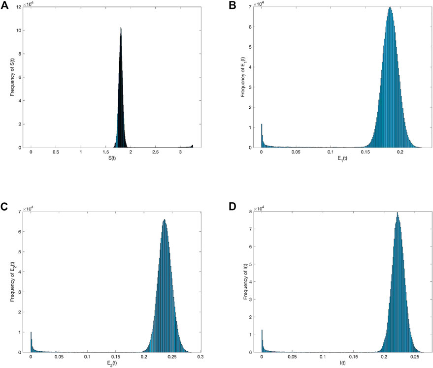
FIGURE 2. Frequency histograms of (A) S(t), (B) E ₁(t), (C) E ₂(t), and (D) I(t) when σ _i (i =1,2)=0.001.

FIGURE 3

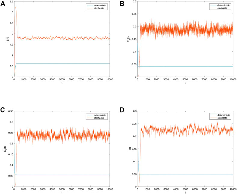
FIGURE 3. Comparison between the deterministic model and stochastic model of the densities of (A) S(t), (B) E ₁(t), (C) E ₂(t), and (D) I(t) change over time when σ _i (i =1,2)=0.001.

Second, the perturbation strength σ is reduced to 0.0001, while all other parameters remain unchanged. Figure 4 depicts the population S(t), E ₁(t), E ₂(t), I(t) probability histogram. Compared to Figure 2, the probabilities obeyed by all populations in the social system are stable, and their distributions have converged in Figure 4. Figure 5 compares the density change trend between deterministic and stochastic systems about population S(t), E ₁(t), E ₂(t), I(t) over time. Even though the perturbation intensity decreases in Figure 5, the stochastic system has greater information spread than the deterministic system. The information spread throughout the social system is not sufficiently stable as it is subject to fluctuations. In other words, information spread in a stochastic system produces fluctuations regardless of changes in perturbation strength. Due to the addition of random environmental factors, the densities of all populations are greater than those spread in a deterministic system.

FIGURE 4

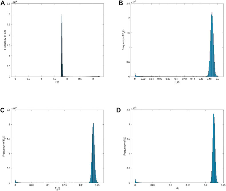
FIGURE 4. Frequency histograms of (A) S(t), (B) E ₁(t), (C) E ₂(t), and (D) I(t) when σ _i (i =1,2)=0.0001.

FIGURE 5

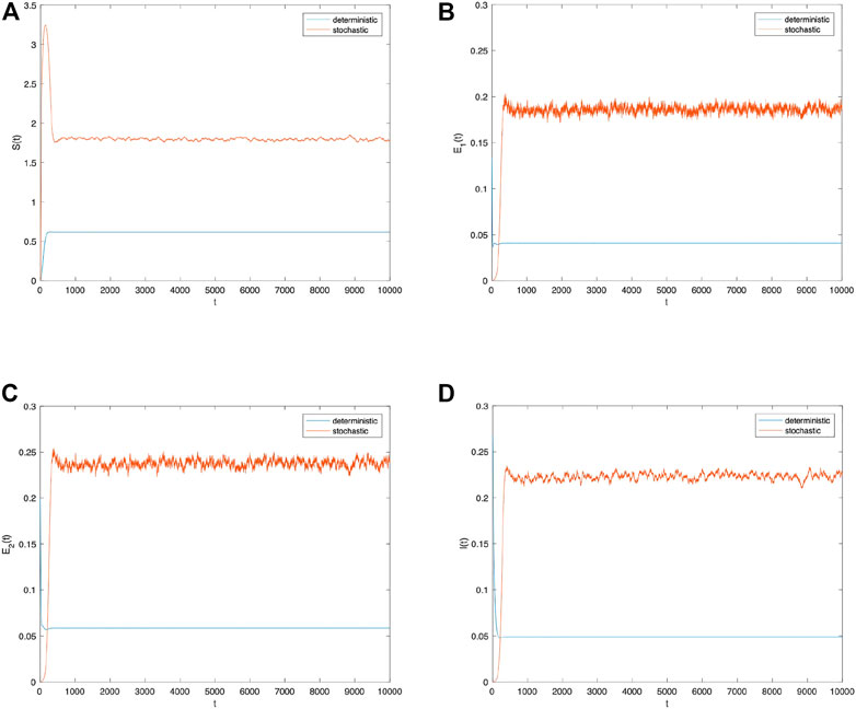
FIGURE 5. Comparison between the deterministic model and stochastic model of the densities of (A) S(t), (B) E ₁(t), (C) E ₂(t), and (D) I(t) change over time when σ _i (i =1,2)=0.0001.

Next, to observe the effects of different perturbation strengths on information spread, the trend plots of information spread over time for the stochastic system with perturbation strengths of 0.001 and 0.0001, respectively, are combined to be analyzed. As shown in Figure 6, as the intensity of the perturbation decreases, the fluctuation of information spread tends to become smoother, indicating that information spreads more easily in systems with random environmental factors and that controlling the random factors in the system can control the fluctuation of information spread effectively.

FIGURE 6

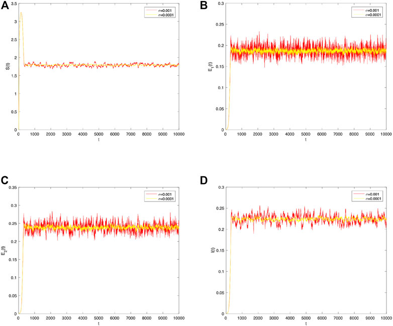
FIGURE 6. Comparison between σ _i (i =1,2)=0.001 and σ _i (i =1,2)=0.0001 of the densities of (A) S(t), (B) E ₁(t), (C) E ₂(t), and (D) I(t) change over time.

Finally, to verify the effect of the control strategy proposed in this chapter, the author kept other parameters constant and observed the density trends of the population E ₁(t) and I(t) over time when the optimal control strategy was used by controlling the stochastic parameters α and β. As shown in Figure 7, when the perturbation strength σ = 0.001, the densities of populations E ₁(t) and I(t) with the optimal control strategy for stochastic parameters α and β are superior to those without a control strategy. As shown in Figure 8, optimal control has a positive effect on information dissemination when the perturbation intensity σ = 0.0001 is reduced further. Furthermore, change the values of other parameters and compare the densities of E ₁(t) and I(t) change trends with different control strategies under different intensities of perturbation. As shown in Figure 9, no matter how the parameter values change, the optimal control strategy proposed in this paper can promote information dissemination effectively. At the same time, adopting optimal control strategies can suppress the fluctuations of information during its spreading.

FIGURE 7

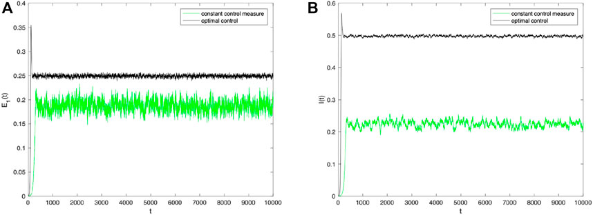
FIGURE 7. Densities of (A) E ₁(t) and (B) I(t) change over time when σ _i (i =1,2)=0.001 under constant control measure and optimal control.

FIGURE 8

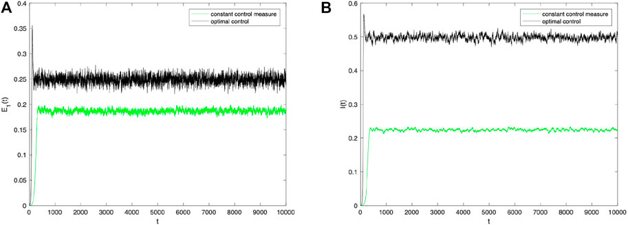
FIGURE 8. Densities of (A) E ₁(t) and (B) I(t) change over time when σ _i (i =1,2)=0.0001 under constant control measure and optimal control.

FIGURE 9

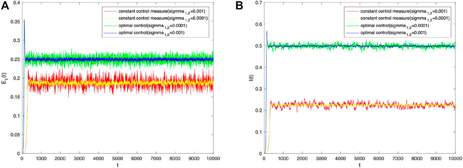
FIGURE 9. Densities of (A) E ₁(t) and (B) I(t) change over time with different intensities of perturbation under constant control measure and optimal control.

According to the results of theoretical analysis and numerical simulation, random factors can promote the dissemination of information. For positive information, it is necessary to fully utilize the random phenomena in the social system to spread beneficial information for social development. For negative information, it is necessary to minimize the interference of random factors on the information to suppress the dissemination of information that is harmful to social development. Technological innovation information plays an important role in the development of enterprises in practical applications [3]. It is usually necessary to leverage the randomness of the social system for technological innovation information, enhance the range of exposure to technological innovation information in society, and promote the random dissemination of technological innovation information among different individuals so as to maximize the diffusion effect. On the contrary, the spread of rumor information hinders the development of society. During the outbreak of COVID-19 all over the world, the rumor that Shuanghuanglian oral liquid could treat COVID-19 was widely spread in China [39], which led to the citizens rushing to purchase the drug and caused social panic. It can be seen from this incident that the continuous emergence of We-media and unscrupulous merchants is a random phenomenon, and effective control of these random phenomena can quickly suppress the spread of rumors.

8 Conclusion

In this paper, stochastic factors in social systems are added to the deterministic model. Then, the stochastic S2EIR model with parameter perturbations is proposed, with two parameters represented by Gaussian white noise: the contact rate of super-spreaders and the conversion rate of information spreaders. The existence of a global positive solution is demonstrated, and sufficient conditions for information disappearance and smooth distribution of information are calculated. In addition, the optimal control strategy for the stochastic model is proposed. The effect of the probability density distribution and white noise perturbation on information dissemination is validated through numerical simulation. The dissemination trends of the information with different perturbation strengths are compared.

From the research presented in this paper, the following conclusions can be drawn: 1) White noise perturbation can promote information dissemination, and random environmental factors play a positive role in information dissemination. 2) As the intensity of perturbation increases, the randomness of the model and the fluctuation of the information spread trend become more obvious. 3) Information spread can be effectively controlled by controlling the stochastic parameters, and the optimal control strategy of this paper is based on the optimal values calculated by the control variables, which is different from previous studies.

There are many uncertainties in the actual social system, and it is more scientific to incorporate these uncertainties into deterministic models in order to develop stochastic models of dissemination. In this paper, the author considers the information spread phenomena of super-spreaders and implicit exposers and uses random perturbation terms to analyze the method of controlling information spread in the actual social system. The results indicate that for positive information, the randomness and complexity of the social system should be utilized to increase the spread of information. In contrast, for negative information, randomness in the social system should be suppressed to the greatest extent possible to limit information dissemination.

Data availability statement

The original contributions presented in the study are included in the article/Supplementary Material; further inquiries can be directed to the corresponding author.

Author contributions

Conceptualization: SK and XH; methodology: SK and YH; software: SK and YH; validation: SK, XH, and HL; formal analysis: SK and YH; investigation: SK and YH; data curation: SK and YH; writing—original draft preparation: SK; and writing—review and editing: XH and HL. All authors listed have made a substantial, direct, and intellectual contribution to the work and approved it for publication.

Funding

This work was supported by the National Natural Science Foundation of China (71472080), the Humanities and Social Sciences Research Projects of the Education Department of Liaoning Province of China (2020LNJC11), and the Natural Science Foundation of Liaoning Science and Technology Agency of China (2022-MS-356).

Conflict of interest

The authors declare that the research was conducted in the absence of any commercial or financial relationships that could be construed as a potential conflict of interest.

Publisher’s note

All claims expressed in this article are solely those of the authors and do not necessarily represent those of their affiliated organizations, or those of the publisher, the editors, and the reviewers. Any product that may be evaluated in this article, or claim that may be made by its manufacturer, is not guaranteed or endorsed by the publisher.

References

1. Pang G, Wang X, Wang L, Hao F, Lin Y, Wan P, et al. Efficient deep reinforcement learning-enabled recommendation. IEEE Trans Netw Sci Eng (2023) 10:871–86. doi:10.1109/TNSE.2022.3224028

CrossRef Full Text | Google Scholar

2. Zhu H, Wang Y, Yan X, Jin Z Research on knowledge dissemination model in the multiplex network with enterprise social media and offline transmission routes. Physica A: Stat Mech its Appl (2022) 587:126468. doi:10.1016/j.physa.2021.126468

CrossRef Full Text | Google Scholar

3. Hu Y, Liu H, Zhao J, Tu L Dynamic analysis of dissemination model of innovation ability of enterprise r&d personnel. Physica A: Stat Mech its Appl (2019) 531:121743. doi:10.1016/j.physa.2019.121743

CrossRef Full Text | Google Scholar

4. Shang Y Lie algebraic discussion for affinity based information diffusion in social networks. Open Phys (2017) 15:705–11. doi:10.1515/phys-2017-0083

CrossRef Full Text | Google Scholar

5. Sun H, Sheng Y, Cui Q An uncertain sir rumor spreading model. Adv Difference Equations (2021) 2021:286. doi:10.1186/s13662-021-03386-w

CrossRef Full Text | Google Scholar

6. Cheng Y, Huo L, Zhao L Dynamical behaviors and control measures of rumor-spreading model in consideration of the infected media and time delay. Inf Sci (2021) 564:237–53. doi:10.1016/j.ins.2021.02.047

CrossRef Full Text | Google Scholar

7. Dong NP, Long HV, Giang NL The fuzzy fractional siqr model of computer virus propagation in wireless sensor network using caputo atangana–baleanu derivatives. Fuzzy Sets Syst (2022) 429:28–59. doi:10.1016/j.fss.2021.04.012

CrossRef Full Text | Google Scholar

8. Daley DJ, Kendall DG Epidemics and rumours. Nature (1964) 204:1118. doi:10.1038/2041118a0

PubMed Abstract | CrossRef Full Text | Google Scholar

9. Chen L, Sun J Global stability of an si epidemic model with feedback controls. Appl Maths Lett (2014) 28:53–5. doi:10.1016/j.aml.2013.09.009

CrossRef Full Text | Google Scholar

10. Cao B, Shan M, Zhang Q, Wang W A stochastic sis epidemic model with vaccination. Physica A: Stat Mech its Appl (2017) 486:127–43. doi:10.1016/j.physa.2017.05.083

CrossRef Full Text | Google Scholar

11. Zaman G, Han Kang Y, Jung IH Stability analysis and optimal vaccination of an sir epidemic model. Biosystems (2008) 93:240–9. doi:10.1016/j.biosystems.2008.05.004

PubMed Abstract | CrossRef Full Text | Google Scholar

12. Efimov D, Ushirobira R On an interval prediction of Covid-19 development based on a seir epidemic model. Annu Rev Control (2021) 51:477–87. doi:10.1016/j.arcontrol.2021.01.006

PubMed Abstract | CrossRef Full Text | Google Scholar

13. Jiang G, Li S, Li M Dynamic rumor spreading of public opinion reversal on weibo based on a two-stage spnr model. Physica A: Stat Mech its Appl (2020) 558:125005. doi:10.1016/j.physa.2020.125005

CrossRef Full Text | Google Scholar

14. Xia Y, Jiang H, Yu Z Global dynamics of ilsr rumor spreading model with general nonlinear spreading rate in multi-lingual environment. Chaos, Solitons and Fractals (2022) 154:111698. doi:10.1016/j.chaos.2021.111698

CrossRef Full Text | Google Scholar

15. Liu Q, Jiang D Dynamics of a multigroup sirs epidemic model with random perturbations and varying total population size. Commun Pure Appl Anal (2020) 19:1089–110. doi:10.3934/cpaa.2020050

CrossRef Full Text | Google Scholar

16. Shang Y Mixed si (r) epidemic dynamics in random graphs with general degree distributions. Appl Maths Comput (2013) 219:5042–8. doi:10.1016/j.amc.2012.11.026

CrossRef Full Text | Google Scholar

17. Zhang Y, Li Y Evolutionary dynamics of stochastic seir models with migration and human awareness in complex networks. Complexity (2020) 2020:1–15. doi:10.1155/2020/3768083

CrossRef Full Text | Google Scholar

18. Liu Q, Jiang D Stationary distribution and probability density for a stochastic seir-type model of coronavirus (Covid-19) with asymptomatic carriers. Chaos, Solitons and Fractals (2023) 169:113256. doi:10.1016/j.chaos.2023.113256

PubMed Abstract | CrossRef Full Text | Google Scholar

19. Hussain G, Khan A, Zahri M, Zaman G Stochastic permanence of an epidemic model with a saturated incidence rate. Chaos, Solitons and Fractals (2020) 139:110005. doi:10.1016/j.chaos.2020.110005

CrossRef Full Text | Google Scholar

20. Wang X, Wang C, Wang K Extinction and persistence of a stochastic sica epidemic model with standard incidence rate for hiv transmission. Adv Difference Equations (2021) 2021:260–17. doi:10.1186/s13662-021-03392-y

CrossRef Full Text | Google Scholar

21. Bobryk R Stability analysis of a sir epidemic model with random parametric perturbations. Chaos, Solitons and Fractals (2021) 143:110552. doi:10.1016/j.chaos.2020.110552

CrossRef Full Text | Google Scholar

22. Kiouach D, Sabbar Y Dynamic characterization of a stochastic sir infectious disease model with dual perturbation. Int J Biomathematics (2021) 14:2150016. doi:10.1142/S1793524521500169

CrossRef Full Text | Google Scholar

23. Li Y, Wei Z Dynamics and optimal control of a stochastic coronavirus (Covid-19) epidemic model with diffusion. Nonlinear Dyn (2021) 109:91–120. doi:10.1007/s11071-021-06998-9

PubMed Abstract | CrossRef Full Text | Google Scholar

24. Danane J, Allali K, Hammouch Z, Nisar KS Mathematical analysis and simulation of a stochastic Covid-19 lévy jump model with isolation strategy. Results Phys (2021) 23:103994. doi:10.1016/j.rinp.2021.103994

PubMed Abstract | CrossRef Full Text | Google Scholar

25. Aslam Noor M, Raza A, Arif MS, Rafiq M, Sooppy Nisar K, Khan I, et al. Non-standard computational analysis of the stochastic Covid-19 pandemic model: An application of computational biology. Alexandria Eng J (2022) 61:619–30. doi:10.1016/j.aej.2021.06.039

CrossRef Full Text | Google Scholar

26. Cheng Y, Huo L, Zhao L Rumor spreading in complex networks under stochastic node activity. Physica A: Stat Mech its Appl (2020) 559:125061. doi:10.1016/j.physa.2020.125061

PubMed Abstract | CrossRef Full Text | Google Scholar

27. Zhang Y, Zhu J Dynamics of a rumor propagation model with stochastic perturbation on homogeneous social networks. J Comput Nonlinear Dyn (2022) 17. doi:10.1115/1.4053269

CrossRef Full Text | Google Scholar

28. Tong X, Jiang H, Chen X, Li J, Cao Z Deterministic and stochastic evolution of rumor propagation model with media coverage and class-age-dependent education. Math Methods Appl Sci n/a (2022) 46:7125–39. doi:10.1002/mma.8959

CrossRef Full Text | Google Scholar

29. Zhou Y, Zhang J, Zhu C, Wang H Modelling and analysis of rumour propagation based on stochastic optimal control. Alexandria Eng J (2022) 61:12869–80. doi:10.1016/j.aej.2022.06.057

CrossRef Full Text | Google Scholar

30. Yue X, Huo L Dynamical behavior of a stochastic sicr rumor model incorporating media coverage. Front Phys (2022) 10. doi:10.3389/fphy.2022.1010428

CrossRef Full Text | Google Scholar

31. Jain A, Dhar J, Gupta V Stochastic model of rumor propagation dynamics on homogeneous social network with expert interaction and fluctuations in contact transmissions. Physica A: Stat Mech its Appl (2019) 519:227–36. doi:10.1016/j.physa.2018.11.051

CrossRef Full Text | Google Scholar

32. Huo L, Dong Y Analyzing the dynamics of a stochastic rumor propagation model incorporating media coverage. Math Methods Appl Sci (2020) 43:6903–20. doi:10.1002/mma.6436

CrossRef Full Text | Google Scholar

33. Mena H, Pfurtscheller L-M, Romero-Leiton JP Random perturbations in a mathematical model of bacterial resistance: Analysis and optimal control. Math Biosciences Eng (2020) 17:4477–99. doi:10.3934/mbe.2020247

PubMed Abstract | CrossRef Full Text | Google Scholar

34. Jiang D, Shi N A note on nonautonomous logistic equation with random perturbation. J Math Anal Appl (2005) 303:164–72. doi:10.1016/j.jmaa.2004.08.027

CrossRef Full Text | Google Scholar

35. Beretta E, Kolmanovskii V, Shaikhet L Stability of epidemic model with time delays influenced by stochastic perturbations. Mathematics Comput Simulation (1998) 45:269–77. doi:10.1016/S0378-4754(97)00106-7

CrossRef Full Text | Google Scholar

36. Du N, Kon R, Sato K, Takeuchi Y Dynamical behavior of lotka–volterra competition systems: Non-autonomous bistable case and the effect of telegraph noise. J Comput Appl Maths (2004) 170:399–422. doi:10.1016/j.cam.2004.02.001

CrossRef Full Text | Google Scholar

37. Lahrouz A, Omari L Extinction and stationary distribution of a stochastic sirs epidemic model with non-linear incidence. Stat Probab Lett (2013) 83:960–8. doi:10.1016/j.spl.2012.12.021

CrossRef Full Text | Google Scholar

38. Mao X Stationary distribution of stochastic population systems. Syst Control Lett (2011) 60:398–405. doi:10.1016/j.sysconle.2011.02.013

CrossRef Full Text | Google Scholar

39. Zhou X, Qiu L, Hao T Scir rumor propagation model with the chord mechanism in social networks. Int J Mod Phys C (2022) 33:2250014. doi:10.1142/S0129183122500140

CrossRef Full Text | Google Scholar