Revealing quantum effects in bosonic Josephson junctions: a multi-configuration atomic coherent state approach

1 Introduction

The Bose–Hubbard (BH) model of S interacting (bosonic) atoms in optical lattices is the basis of many state-of-the-art experimental [1–4] and theoretical efforts [3, 5, 6]. The cold atom Hubbard tool box introduced in [5] puts a focus on strongly interacting many-body dynamics and embraces the fields of quantum optics, quantum computation, and solid-state physics. The BH model is a paradigm for the rich physical phenomena exhibited in these areas, such as quantum phase transitions between the superfluid and the Mott insulator phase [1], self-trapping in bosonic Josephson junctions [7], and quantum chaology [6].

Restricting the amount of lattice sites makes the quantum dynamics of the BH model easily tractable numerically for moderate particle numbers. A recent theoretical work has thus focused on the cases of four (and six) sites [8] with different levels of approximation: exact, semi-classical, and classical (mean-field or truncated Wigner approximation (TWA)). In addition, the trimer (ring) case has been studied because it leads to the melting of discrete vortices via quantum fluctuations [9] and that it is the smallest system that displays a mixed phase-space mean-field dynamics without an external driving term [10, 11]. This system has also been dealt with using a group theoretical [12, 13] and a semi-classical time-domain approach [14]. With an additional drive (periodic kicks), even the double-well case is showing signs of chaos [15]. Furthermore, the case of two wells without external driving has been extensively studied. The system dynamics has, for example, been investigated both in a mean-field classical approximation and fully (and perturbatively) quantum mechanically [7, 16–20], as well as also semiclassically, using a phase-space picture [21], or employing the Herman–Kluk propagator [14, 22]. This same propagator has also been used in a semi-classical time-domain study of the single-well problem [23]. Furthermore, the driven single-well problem has served as a model in a study of dynamical tunneling [24].

An important lesson from the vast literature is that semi-classical approaches do well in reproducing the full quantum results, while the mean-field and truncated Wigner method have their limitations. The TWA does not allow for the investigation of revival phenomena, present in quantum dynamics [20]. In contrast, the macroscopic quantum self trapping effect in bosonic Josephson junctions could already be uncovered using a mean-field approach based on the Gross-Pitaevskii equation [7]. However, it turns out that mean-field theory predicts the transition to macroscopic quantum self-trapping at too large values of the on-site interaction strength[25].

In the following, we will focus on the quantum dynamics in the case of two wells, for which the direct experimental observation of tunneling and self-trapping has become possible [26]. Theoretically, this case has been reviewed in [27] as well as in [28], where the exact solubility of the eigenvalue problem in terms of the Bethe-Ansatz has been reviewed. Furthermore, a novel insight on finite size (i.e., finite particle number) effects in the mean-field dynamics of those Josephson junction systems has been given by Wimberger et al. [25]. These authors have used a so-called atomic or SU(2) generalized coherent state [29] to uncover mean-field 1/S corrections to the more familiar mean-field results based on standard Glauber coherent states. We will also employ those favorable number conserving SU(2) states here. However, we will not use them from the perspective of the mean-field, where just a single state is taken to solve the time-dependent Schrödinger equation (TDSE). In contrast, we will investigate the consequences of non-trivial multiplicity, which has first been chosen to be just 2, i.e., we will use a superposition of two SU(2) states to solve the TDSE. Inspired by the previous experience with Gaussian-based approaches to solve the TDSE for molecular Hamiltonians [30, 31], as well as for spin-boson-type problems [32–34], and due to the entanglement entropy studies in [35] using two SU(2) states, we are confident that only a handful of suitable time-dependent basis states could be enough to achieve satisfactory agreement with exact quantum solutions if a full-fledged variational approach is taken. In order to correctly account for more demanding quantum effects like self-trapping, the multiplicity has to be increased, but it can still be kept below the total number of time-independent Fock states that has to be used in a full quantum calculation. Furthermore, it is expected that the number of quantum trajectories needed for convergence will be much reduced as compared to that of semiclassical trajectory calculations that are based on multiple mean-field trajectories.

The study is structured as follows. In Section 2, we briefly review the mean-field approach, based on a single atomic coherent state (ACS), to the dynamics of the bosonic Josephson junction. At the end of this section, a special focus will be given on the stability analysis of the non-linear classical phase-space dynamics. In Section 3, we then choose an ansatz wave-function with non-trivial multiplicity, employing a small number of time-evolving atomic coherent states to represent the quantum beat dynamics (collapse and revival of population imbalance) of the BH dimer. In a brief review of the quantum phase operator concept, we establish the relation between the phase difference in the mean-field approach and its quantum analog. This allows us to compare numerical results for phase-space trajectories with the corresponding solution of the TDSE. We will cover a broad range of system parameters as well as initial conditions. It is observed that there are cases, close to the equilibrium point of the classical dynamics, in which just two ACSs will suffice to achieve reasonable agreement with the exact results. However, at a larger distance from the equilibrium point of classical dynamics, the number of ACS will have to be increased. In Section 4, we give conclusions and an outlook on possible future work. Methodological details can be found in Section 5.

2 Two-site BH model and mean-field dynamics

2.1 The Hamiltonian

The simplest Hamiltonian for the bosonic Josephson junction (two-site BH model) in normal ordered form reads

$\widehat{H}=-J\left({\widehat{a}}_1^{†}{\widehat{a}}_2+{\widehat{a}}_2^{†}{\widehat{a}}_1\right)+\frac{U}{2}{\displaystyle \sum _{j=1}^2}{\widehat{a}}_j^{†2}{\widehat{a}}_j^2,(1)$

where the bosonic ladder operators ${\widehat{a}}_j$ and ${\widehat{a}}_j^{†}$ with the commutation relation $[{\widehat{a}}_j,{\widehat{a}}_j^{†}]=\widehat{1}$ annihilate or create, respectively, a particle (a bosonic atom) in the site labeled by the index j. Furthermore,

${\widehat{n}}_j={\widehat{a}}_j^{†}{\widehat{a}}_j,j=\mathrm{1,2},(2)$

counts the number of particles per site and $\widehat{S}={\widehat{n}}_1+{\widehat{n}}_2$ is the total number-operator, and its expectation value S is a conserved quantity because $\widehat{S}$ commutes with $\widehat{H}$.

The (dimensionless) parameters U and J > 0 denote the strength of the on-site interaction, determined by the s-wave scattering length of the atomic species considered, and the tunneling amplitude, respectively. Later on, we will consider positive and negative values of U, corresponding to repulsive and attractive interaction between the atoms, respectively.

2.2 Mean-field dynamics

The evolution of the BH model is governed by the TDSE

$\mathrm{i}|\dot{\mathrm{\Psi }}\left(t\right)\rangle =\widehat{H}|\mathrm{\Psi }\left(t\right)\rangle ,(3)$

for the wave-function |Ψ(t)⟩. Here, as well as in the remainder of this paper, we have set ℏ = 1. In order to solve for the dynamics, in the present section, we will be closely following the mean-field work presented in [25].

We start the discussion by recalling the eigenvalue equation of the annihilation operator in the form

${\widehat{a}}_j|{\alpha }_j\left(t\right)\rangle ={\alpha }_j\left(t\right)|{\alpha }_j\left(t\right)\rangle =\sqrt{n_j\left(t\right)}{\mathrm{e}}^{\mathrm{i}{\varphi }_j\left(t\right)}|{\alpha }_j\left(t\right)\rangle ,(4)$

with the time-dependent Glauber coherent state [36] (displacement operator applied to the ground state)

$|{\alpha }_j\left(t\right)\rangle ={\mathrm{e}}^{-|{\alpha }_j\left(t\right){|}^2/2}{\alpha }_j(t){\widehat{a}}_j^{†}|0\rangle ,(5)$

and time-dependent average particle number n_j(t) and phase ϕ_j(t) of the site indexed by j. The position space representation of this state is a displaced Gaussian wave-function [30].

The approximate mean-field dynamics can then be obtained by using an ansatz in terms of a single ACS [29], defined by

$\begin{array}{ccc}\hfill |\mathrm{\Psi }\left(t\right)\rangle & =\hfill & \frac{1}{\sqrt{S!}}{\left(\sqrt{\frac{1+z\left(t\right)}{2}}{\widehat{a}}_1^{†}+\sqrt{\frac{1-z\left(t\right)}{2}}{e}^{-\mathrm{i}\varphi \left(t\right)}{\widehat{a}}_2^{†}\right)}^S|\mathrm{0,0}\rangle \hfill \\ \hfill & =\hfill & |S,\sqrt{\frac{1+z\left(t\right)}{2}},\sqrt{\frac{1-z\left(t\right)}{2}}{e}^{-\mathrm{i}\varphi \left(t\right)}\rangle .\hfill \end{array}(6)$

Here, |0, 0⟩ is a shorthand notation for the direct product of two single-particle vacuum states, and the time-dependent parameters

$z\left(t\right)=\frac{n_1\left(t\right)-n_2\left(t\right)}{S},(7)$

and

$\varphi \left(t\right)={\varphi }_1\left(t\right)-{\varphi }_2\left(t\right),(8)$

are the (normalized) population imbalance and the relative phase of the two sites, respectively [25]. The time-dependent particle number expectations at site j can take on fractional values. As a simple example, we consider the case of S = 2 and initial z(0) = 1/2, for which n₁(0) = 3/2 and n₂(0) = 1/2.

If the system dynamics is governed by a harmonic oscillator Hamiltonian or a Rabi model (single harmonic mode coupled to a spin system), the use of the Glauber coherent states mentioned previously is common [37, 38]. In the present case, we opt for using the generalized coherent states (GCSs) [39, 40], which for two modes are the ACS introduced above, instead of a direct product of Glauber coherent states. This is because the former are better suited to describe particle number conserving dynamics, as the latter consist of a superposition of number states in the general case [41, 42]. For Bose–Einstein condensates (BECs), this observation has also been made by Schachenmayer et al. [43], who showed that the multi-well Glauber coherent state ansatz is equivalent to the GCS ansatz only in the case of large particle numbers. Furthermore, it is worthwhile to note that the highly entangled GCS is the ground state of the “free-boson” model, i.e., the BH model with vanishing on-site interaction, U = 0 [7, 44–46].

The representation of the ACS in the last line in Eq. 6 is motivated by the general expression of a multimode generalized coherent state (total number of modes given by M) in the form [47]

$|S,\vec{\xi }\rangle =\frac{1}{\sqrt{S!}}{\left({\displaystyle \sum _{i=1}^M}{\xi }_i{a}_i^{†}\right)}^S|\mathrm{0,0},\dots ,0\rangle ,(9)$

where the entries of the vector $\vec{\xi }$ are the complex parameters {ξ_i}, which obey the “normalization” condition ${\sum }_{i=1}^M|{\xi }_i{|}^2=1$. The representation of the unit operator in these states has been used in [48]to establish an exact variational dynamics of the multi-mode BH model. The number of independent real parameters of the GCS in the two-site case, M = 2, is 3 (two complex numbers minus the normalization condition mentioned previously) but there is an overall phase factor that is irrelevant, however, so that we just remain with the two real parameters z and ϕ introduced previously. In the case of arbitrary site numbers, the equations for the parameters ξ_i are referred to as discrete non-linear Schrödinger equations, which can be viewed as the discrete analog of the Gross–Pitaevskii equation for a BEC [6].

In the remainder of this study, we will focus on the Josephson junction case. The mean-field equations for the real parameters z(t) and ϕ(t) are given by [25]:

$\dot{z}=2J\sqrt{1-z^2}\sin \varphi ≔f_1,(10)$

$\dot{\varphi }=-2J\frac{z}{\sqrt{1-z^2}}\cos \varphi -U\left(S-1\right)z≔f_2,(11)$

which are equations of motion of non-rigid pendulum type [49–51]. A stationary solution of these coupled nonlinear equations is given by the equilibrium points (0, 2πn) with n = 0, ±1, ±2, ….

In the next step, we linearize the system of equations around one of the equilibrium points. The Jacobian matrix [52] at (z*, ϕ*) = (0, 0) is given by

$\mathbf{J}=\left(\begin{array}{cc}\hfill {\left.\frac{\partial f_1}{\partial z}\right|}_{z^{*},{\varphi }^{*}}\hfill & \hfill {\left.\frac{\partial f_1}{\partial \varphi }\right|}_{z^{*},{\varphi }^{*}}\hfill \\ \hfill {\left.\frac{\partial f_2}{\partial z}\right|}_{z^{*},{\varphi }^{*}}\hfill & \hfill {\left.\frac{\partial f_2}{\partial \varphi }\right|}_{z^{*},{\varphi }^{*}}\hfill \end{array}\right)=\left(\begin{array}{cc}\hfill 0\hfill & \hfill 2J\hfill \\ \hfill -2J-\left(S-1\right)U\hfill & \hfill 0\hfill \end{array}\right),(12)$

and its eigenvalues are

${\lambda }_{\pm }=\pm \sqrt{2}J\sqrt{-2+\frac{U}{J}-\frac{US}{J}}.(13)$

The so-called strength parameter

$\mathrm{\Lambda }=U\left(S-1\right)/\left(2J\right),(14)$

is an appropriate parameter combination to be used frequently in the following section. More details on the linearized mean-field equations around the stationary points can be found in Section 5.1.

A qualitative change in the mean-field dynamics will occur when the radicand in Eq. 13 changes sign, which happens at the critical value Λ_SSB = −1, where the index SSB stands for spontaneous symmetry breaking [45]. If Λ > − 1, both eigenvalues are imaginary, which indicates that the aforementioned equilibrium point is a stable one and the solution is symmetric around the origin, whereas Λ < − 1 will lead to the emergence of another class of stable equilibrium points. The symmetry breaking solutions are located around the new stationary point(s)

$\left(z^{\text{SSB}},{\varphi }^{\text{SSB}}\right)=\left(\pm \sqrt{1-\frac{1}{{\mathrm{\Lambda }}^2}},2\pi n\right),(15)$

of the system of Eqs 10, 11, where $n\in \mathbb{Z}$ [25]. The corresponding Jacobian matrix is

$\mathbf{J}=\left(\begin{array}{cc}\hfill 0\hfill & \hfill \frac{2J}{\sqrt{{\mathrm{\Lambda }}^2}}\hfill \\ \hfill -2J\mathrm{\Lambda }\left(1+\mathrm{\Lambda }\sqrt{{\mathrm{\Lambda }}^2}\right)\hfill & \hfill 0\hfill \end{array}\right),(16)$

and its eigenvalues are

${\lambda }_{\pm }=\pm \frac{2J\sqrt{-{\mathrm{\Lambda }}^4-\mathrm{\Lambda }\sqrt{{\mathrm{\Lambda }}^2}}}{\sqrt{{\mathrm{\Lambda }}^2}}.(17)$

If Λ < − 1, these are imaginary and the solution of the linearized equations around the SSB points is oscillatory. Both cases are displayed in Figure 1, with the left panel showing motion around the stable fixed point for U/J = 0.1 and the right panel showing the trajectories in case of U/J = −0.12, where the stable fixed point at the origin has turned into an unstable one and new stable fixed points appear at positive and negative values of z. For an experimental realization of this scenario, see [53]. In Section 5.1, an analytic expression for the linearized solution in panel B of Figure 1 at small values of z and ϕ is given.

FIGURE 1

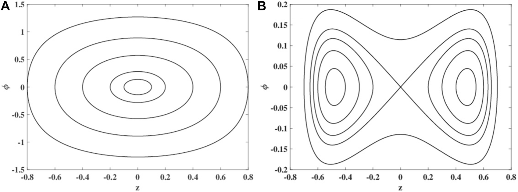
FIGURE 1. Phase-space trajectories from the mean-field dynamics for different initial conditions and different values of on-site interaction strength: (A) U/J = 0.1 and (B) U/J = −0.12. The number of particles is S = 20 in both cases.

In [25], it is shown that the mean-field prediction for the onset of SSB based on single Glauber coherent states fails dramatically at small particle numbers. The mean-field result based on a single SU(2) coherent state does better than the Glauber state prediction at small S but is not exact. However, both mean-field predictions reproduce the full quantum result more faithfully at large values of S, as can be seen in Figure 4 of [25].

It can be further concluded from the mean-field Eqs 10, 11 that the quantity

$E=\frac{US}{4}\left(S-1\right)z^2-JS\sqrt{1-z^2}\cos \varphi ,(18)$

is a constant of motion [25]. This leads to the existence of a parameter regime, in which the imbalance cannot become 0 during an oscillation cycle and, therefore, the average value of z will be non-zero. The condition for this macroscopic quantum self-trapping (MQST) effect is E(z(0), ϕ(0)) > E(0, π) = JS. In terms of the strength parameter introduced previously, the onset of self-trapping is at [54]

${\mathrm{\Lambda }}_{\text{MQST}}=\frac{1+\sqrt{1-z^2\left(0\right)}\cos \varphi \left(0\right)}{z^2\left(0\right)/2},(19)$

depending strongly on the initial position in phase space. In contrast to the case of SSB, the mean-field MQST effect sets in at too large positive values of U (repulsive interaction), whereas the mean-field theory predicts the onset of SSB at too small values of |U| [25].

3 Beyond mean-field dynamics

Due to the shortcomings of the mean-field approach for U ≠ 0, like the absence of collapses and revivals of population imbalance [17], as well as failures in the prediction of the onset of MQST as well as SSB [25], we will now go beyond the mean-field approach by employing a multi-configuration ansatz for the solution of the TDSE.

We first give an explicit derivation of the equations of motion followed by a brief review of the phase operator concept, which is needed to display our quantum results. The parameter regimes of the results to be presented are given in Table 1, from which it can be inferred that we select parameters bordering, as well as inside the Josephson regime (1 < Λ < S²), intermediate between the Rabi and Fock regimes [27], for which Λ ≪ 1 and Λ ≫ S², respectively. In the Josephson regime, the parameters we chose lead from simple to more complex collapse and revival dynamics, with increasing breathing amplitude, to the phenomena of MQST and SSB, mentioned in the previous section. The Rabi regime is considered to be the most trivial of the three commonly studied regimes, while the Fock regime cannot be described reliably by our approach.

TABLE 1

TABLE 1. Hamiltonian and initial state parameters to be investigated in detail in Section 3. The initial phase was zero in all cases. PO: plasma oscillation, MQST: macroscopic quantum self trapping, and SSB: spontaneous symmetry breaking.

3.1 Equations of motion

As a step toward the exactness of the solution, we replace the wave-function of Eq. 6 by a linear combination of N time-dependent SU(2) coherent states, written as in the general SU(M) case of Eq. 9, leading to

$|\mathrm{\Psi }\left(t\right)\rangle ={\displaystyle \sum _{k=1}^N}{A}_k\left(t\right)|S,{\xi }_{k1}\left(t\right),{\xi }_{k2}\left(t\right)\rangle .(20)$

We stress that all the parameters, compactly written as vectors A (with N entries) and ξ (with 2N entries), are time-dependent and complex-valued. Their (non-linear) equations of motion, again derived from the TDVP, in the general case of arbitrary multiplicity N as well as the site number M, have been given in matrix form in the appendix of [48].

For being self-contained, here, we explicitly review the variational procedure for the double-well problem. With the trial state from Eq. 20 the Lagrangian $L≔\mathrm{i}⟨\mathrm{\Psi }|{\partial }_t|\mathrm{\Psi }⟩-⟨\mathrm{\Psi }|\widehat{H}|\mathrm{\Psi }⟩$ takes the explicit form

$\begin{array}{ll}\hfill L& ={\displaystyle \sum _{k,j=1}^N}{A}_k^{*}{\dot{A}}_j\langle {\vec{\xi }}_k|{\vec{\xi }}_j\rangle +iS{\displaystyle \sum _{k,j=1}^N}{A}_k^{*}{A}_j{\displaystyle \sum _{i=1}^2}{\xi }_k^{*}{\dot{\xi }}_{ji}\langle \overrightarrow{{\xi }_k^{\prime }}|\overrightarrow{{\xi }_j^{\prime }}\rangle \hfill \\ \hfill & -{\displaystyle \sum _{k,j=1}^N}{A}_k^{*}{A}_j\left[-JS\left({\xi }_{k1}^{*}{\xi }_{j2}+{\xi }_{k2}^{*}{\xi }_{j1}\right)\langle \overrightarrow{{\xi }_k^{\prime }}|\overrightarrow{{\xi }_j^{\prime }}\rangle \right.\hfill \\ \hfill & \left.+\frac{U}{2}S\left(S-1\right)\left({\xi }_{k1}^{*2}{\xi }_{j1}^2+{\xi }_{k2}^{*2}{\xi }_{j2}^2\right)\langle \overrightarrow{{\xi }_k^{\prime \prime }}|\overrightarrow{{\xi }_j^{\prime \prime }}\rangle \right].\hfill \end{array}(21)$

The corresponding Euler-Lagrange equations are given by

$\frac{\partial L}{\partial u_k^{*}}-\frac{\mathrm{d}}{\mathrm{d}t}\frac{\partial L}{\partial {\dot{u}}_k^{*}}=0,(22)$

where u_k denotes one element of the set {A_k, ξ_k1, ξ_k2} of 3N complex valued parameters in |Ψ⟩. For the coefficients, this leads to the equations of motion

$\mathrm{i}{\displaystyle \sum _{j=1}^N}{\dot{A}}_j\langle \overrightarrow{{\xi }_k}|\overrightarrow{{\xi }_j}\rangle +iS{\displaystyle \sum _{j=1}^N}{A}_j{\displaystyle \sum _{i=1}^2}{\xi }_{ki}^{*}{\dot{\xi }}_{ji}\langle \overrightarrow{{\xi }_k^{\prime }}|\overrightarrow{{\xi }_j^{\prime }}\rangle -\frac{\partial H}{\partial A_k^{*}}=0,(23)$

where

$\frac{\partial H}{\partial A_k^{*}}={\displaystyle \sum _{j=1}^N}{A}_j\left[-JS\left({\xi }_{k1}^{*}{\xi }_{j2}+{\xi }_{k2}^{*}{\xi }_{j1}\right)\langle \overrightarrow{{\xi }_k^{\prime }}|\overrightarrow{{\xi }_j^{\prime }}\rangle +\frac{U}{2}S\left(S-1\right){\displaystyle \sum _{i=1}^2}{\xi }_{ki}^{*2}{\xi }_{ji}^2\langle \overrightarrow{{\xi }_k^{\prime \prime }}|\overrightarrow{{\xi }_j^{\prime \prime }}\rangle \right].(24)$

For the coherent state parameters ξ_jm (m = 1, 2), we get

$\begin{array}{ll}\hfill & \mathrm{i}S\left[{\displaystyle \sum _{j=1}^N}{A}_k^{*}{\dot{A}}_j{\xi }_{jm}⟨\overrightarrow{{\xi }_k^{\prime }}|\overrightarrow{{\xi }_j^{\prime }}⟩+{\displaystyle \sum _{j=1}^N}{A}_k^{*}{A}_j{\dot{\xi }}_{jm}⟨\overrightarrow{{\xi }_k^{\prime }}|\overrightarrow{{\xi }_j^{\prime }}⟩\right.\hfill \\ \hfill & +\left.\left(S-1\right){\displaystyle \sum _{j=1}^N}{A}_k^{*}{A}_j{\displaystyle \sum _{i=1}^2}{\xi }_{ki}^{*}{\dot{\xi }}_{ji}{\xi }_{jm}⟨\overrightarrow{{\xi }_k^{\prime \prime }}|\overrightarrow{{\xi }_j^{\prime \prime }}⟩\right]-\frac{\partial H}{\partial {\xi }_{km}^{*}}=0,\hfill \end{array}(25)$

where

$\begin{array}{ll}\hfill \frac{\partial H}{\partial {\xi }_{k1}^{*}}& ={\displaystyle \sum _{j=1}^N}{A}_k^{*}{A}_j\left[-JS{\xi }_{j2}\langle \overrightarrow{{\xi }_k^{\prime }}|\overrightarrow{{\xi }_j^{\prime }}\rangle -JS\left(S-1\right)\left({\xi }_{k1}^{*}{\xi }_{j2}+{\xi }_{k2}^{*}{\xi }_{j1}\right){\xi }_{j1}\langle \overrightarrow{{\xi }_k^{\prime \prime }}|\overrightarrow{{\xi }_j^{\prime \prime }}\rangle \right.\hfill \\ \hfill & +\left.US\left(S-1\right){\xi }_{k1}^{*}{\xi }_{j1}^2\langle \overrightarrow{{\xi }_k^{\prime \prime }}|\overrightarrow{{\xi }_j^{\prime \prime }}\rangle +\frac{U}{2}S\left(S-1\right)\left(S-2\right){\displaystyle \sum _{i=1}^2}{\xi }_{ki}^{*2}{\xi }_{ji}^2{\xi }_{j1}\langle \overrightarrow{{\xi }_k^{\prime \prime \prime }}|\overrightarrow{{\xi }_j^{\prime \prime \prime }}\rangle \right],\hfill \end{array}(26)$

and an analogous equation for the second index being 2.

Some numerical tricks to solve the highly non-linear, implicit equations of motion in Eqs 23, 25 have been devised in [55] for the case of Glauber coherent basis state functions. Because of the restriction to M = 2 of the site number in the present investigation, at least for moderate particle numbers, the TDSE can also be solved easily by an expansion of the wave-function in (time-independent) Fock states, whose coefficients fulfill a (numerically more well-behaved) system of coupled linear first-order differential equations. The number of Fock states required is determined by the particle number via S + 1. More details on the full quantum (Fock space) calculations, whose results will be referred to as exact quantum results, are given in Section 5.1.

We stress that in all exact and beyond mean-field calculations to be presented, we take a single ACS as the initial condition of the dynamics. For the beyond mean-field calculations, this means that a single element out of the set {A_k} is non-zero initially, whereas all other elements will take non-zero values only in the course of time.

3.2 Brief review of phase operator concept

From the wave-function given by Eq. 20, we can calculate the time-dependent site populations by taking expectation values of the operators from Eq. 2, and from this the imbalance z between the two sites. For the analog of the relative phase ϕ, we use the quantum phase operator concept [9, 56], leading to the expectation values

$⟨\cos \widehat{\varphi }⟩=\frac{⟨{\widehat{a}}_2^{†}{\widehat{a}}_1+{\widehat{a}}_2{\widehat{a}}_1^{†}⟩}{\sqrt{2⟨2{\widehat{n}}_1{\widehat{n}}_2+{\widehat{n}}_1+{\widehat{n}}_2⟩}},(27)$

$⟨\sin \widehat{\varphi }⟩=\frac{\mathrm{i}⟨a_1^{†}{a}_2-a_2^{†}{a}_1⟩}{\sqrt{2⟨2{\widehat{n}}_1{\widehat{n}}_2+{\widehat{n}}_1+{\widehat{n}}_2⟩}},(28)$

$⟨{\sin }^2\widehat{\varphi }⟩=\frac{1}{2}-\frac{⟨{\left({\widehat{a}}_2^{†}{\widehat{a}}_1\right)}^2+{\left({\widehat{a}}_2{\widehat{a}}_1^{†}\right)}^2⟩}{2⟨2{\widehat{n}}_1{\widehat{n}}_2+{\widehat{n}}_1+{\widehat{n}}_2⟩},(29)$

of the cosine and sine of the phase operator and its sine square. In addition, the variance of the sine is defined by

$\mathrm{\Delta }\left(\sin \widehat{\varphi }\right)≔\langle {\sin }^2\widehat{\varphi }\rangle -\langle \sin {\widehat{\varphi }\rangle }^2.(30)$

The normalization condition $⟨{\sin }^2\widehat{\varphi }+{\cos }^2\widehat{\varphi }⟩=1$ and the expectation of ${\cos }^2\widehat{\varphi }$ from [9] have been used to derive Eq. 29.

The relation between the sine of the classical phase variable, displayed in Figure 1, and the expectation of the sine of the quantum phase is

$⟨\sin \widehat{\varphi }⟩=\frac{S\sqrt{1-z^2}}{\sqrt{S\left(S-1\right)\left(1-z^2\right)+2S}}\sin \varphi ,(31)$

as can be derived by applying the operator in Eq. 28 to an ACS. For S → ∞, the prefactor on the RHS of the aforementioned equation becomes unity and the quantum and classical expressions become identical. Furthermore, in [9] it has been shown that the melting of coherence between the two sites is mirrored by the vanishing of the expectation of $\cos \widehat{\varphi }$ and the occurrence of large fluctuations of the corresponding variance.

In the following section, we will focus on parameters on the border and inside of the most interesting regime, the so-called Josephson regime [27]. Depending on the initial conditions, beyond mean-field effects can be observed in this case. In addition, we will also allow for negative values of the strength parameter Λ smaller than −1, in order to study the SSB case and will use large positive Λ values close to the (mean-field) MQST regime.

3.3 Plasma oscillations

In the following section, we first consider the case of a small on-site interaction. In addition, the initial imbalance shall first be small. In the second step, this imbalance shall be large at t = 0.

3.3.1 Small initial population imbalance

For small values of U and z, we only include two ACS in the ansatz in Eq. 20, i.e., we use N = 2. Initially, ξ can be still be parameterized in analogy to the procedure of the previous section by $({\xi }_{11},{\xi }_{12})=(\sqrt{\frac{1+z_1}{2}},\sqrt{\frac{1-z_1}{2}}{e}^{-i{\varphi }_1})$ and $({\xi }_{21},{\xi }_{22})=(\sqrt{\frac{1+z_2}{2}},\sqrt{\frac{1-z_2}{2}}{e}^{-i{\varphi }_2})$. To highlight the changes that the inclusion of an additional basis state leads to, for the first SU(2) state, we use three different initial conditions, namely, z₁ ∈ {0.01, 0.05, 0.1}, ϕ₁ = 0, A₁ = 1. For the second SU(2) state, the initial values are identical and are fixed as z₂ = 0, ϕ₂ = 2π/3, A₂ = 0.

The phase-space trajectories in three different levels of approximation and for the three different initial conditions are shown in Figure 2, for S = 20 and an on-site interaction strength of U = 0.1J, implying US/(2J) = 1. We stress that the expectation value of the sine of the phase operator is plotted on the y-axis. Its relation to the sine of the phase difference in the mean-field case is given in Eq. 31.

FIGURE 2

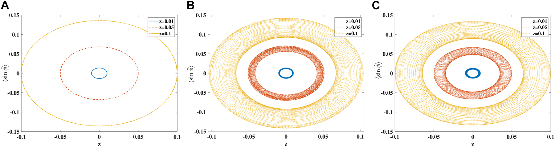
FIGURE 2. Phase-space trajectories in: (A) mean-field, (B) beyond mean-field using ACS with N = 2, and (C) exact quantum dynamics. Different initial conditions are indicated by different line styles: z = 0.01 (solid blue), z = 0.05 (dashed red), and z = 0.1 (dash-dotted yellow). System parameters are U/J = 0.1 and S = 20.

In mean-field approximation, displayed in panel A of Figure 2, all the three initial conditions give rise to an ellipsoidal phase space pattern as shown in the previous section. Going beyond the mean-field approach by allowing for just one additional ACS, we see a qualitatively different behavior, displayed in panel B of Figure 2, which corresponds to a beating of the population imbalance, here displayed by a spiraling motion that first moves inward and then outward for all three initial conditions. This is shown not to be an artifact by comparison to the full quantum solution, displayed in panel C of Figure 2, which exhibits an almost quantitative agreement with the ACS solution of multiplicity 2. We stress that the choice of the initial phase of the second ACS is decisive for the quality of our beyond mean-field results. Choosing ϕ₂ to be 0, e.g., would lead to a spiraling in the wrong direction.

In the case of the smallest imbalance displayed in Figure 2, the beating amplitude (the width of the blue ring) is the smallest and the description of the quantum dynamics with a single classical (mean-field) trajectory is almost adequate, as it would be in the Rabi-oscillation regime, in which Λ ≪ 1, a case we are not considering herein. However, as shown in [14], in order to cope with the collapse and revival of the population imbalance oscillations, a multitude of classical trajectories is needed. A ballpark number for the sample size in the Monte-Carlo integrations performed by Simon and Strunz is 10⁴. The TWA based on a similar sampling procedure does not capture the revival oscillations, but a full-fledged semiclassical approach is required to this end. To put our work in context, we stress that to capture the quantum behavior displayed in Figure 2 almost quantitatively, we need only two “trajectories,” i.e., two ACSs. This dramatic reduction in the basis size is due to the fact that in our present case, also the trajectories (the dynamical evolution of the basis function parameters) undergo the full variational procedure, i.e., they are not mean-field trajectories. We are thus losing the intuitive appeal of a semiclassical method at the benefit of much lesser computational effort, although the calculation of the quantum trajectories is more involved than that of the mean-field ones. In summary, we note that in a comparison of the hierarchy of variational methods based on Glauber coherent states, applied to the anharmonic Morse potential in [30], the reduction in basis function size was counteracted by the (numerical) complexity of the solution of the variational equations of motion.

3.3.2 Large initial population imbalance

The small initial imbalance in the previous case has led to an incomplete collapse, i.e., the oscillation amplitude was still rather large in all the three cases at all times, with only small beating amplitude. In order to suppress the total oscillation amplitude, i.e., to see very small oscillations at least temporarily, we have to allow for larger initial imbalances, which will be carried out next. For the case of U = 0.1J and with initial z = 0.5, the exact quantum dynamics for two different total particle numbers, S = 20 and S = 50, is shown in Figure 3. Corresponding mean-field calculations (not shown) would display a closed single-loop oscillation without any spiraling in (decrease of the oscillation amplitude). In the quantum case, however, we see an almost complete collapse of the amplitude, the larger the particle number. For the larger S, in addition, the population imbalance and the expectation of the sine of the phase operator are 0 for a longer time (see also Figure 4).

FIGURE 3

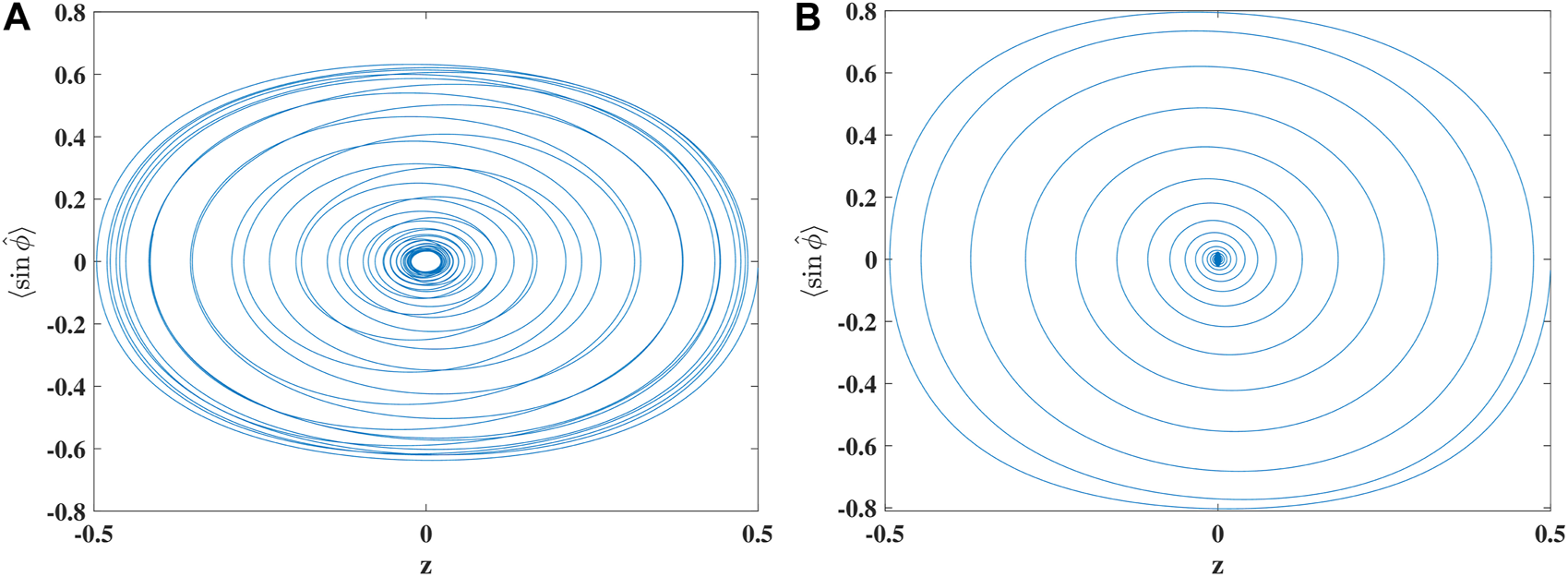
FIGURE 3. Exact quantal phase-space trajectories for times up to Jt = 100 in the case U/J = 0.1 for (A) S = 20 and (B) S = 50. The initial condition is z = 0.5 in both cases.

FIGURE 4

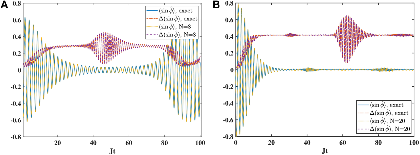
FIGURE 4. Comparison of beyond mean-field and exact quantum results for (A) S = 20 and (B) S = 50. The initial condition is z = 0.5, ϕ = 0 in both cases. The system parameter is U/J = 0.1. The expectation values of the sine of the phase (exact results: solid blue line and multi ACS results: dotted yellow line) and its variance (exact results: dash-dotted red line and multi ACS results: dashed purple line) are displayed.

In Figure 4, we display the time evolution of the sine of the phase operator and its variance. The results of the beyond mean-field approach and exact quantum calculations are compared. First, we observe the collapse and revival in the case of S = 20. For S = 50, the maximum time considered is too short to observe the revival. In addition, we can see that the suppression of the oscillation amplitude of $⟨\sin \widehat{\varphi }⟩$ comes along with an increase in the amplitude of variance oscillation. Furthermore, agreement almost within line thickness between the exact and ACS results can be achieved, but only if the multiplicity is increased considerably compared to the previous case of small initial imbalance. The multiplicities needed are N = 8 in the case of S = 20 and N = 20 in the case of S = 50. The occurrence of large amplitude oscillations in the variance has to be accounted for by an increase in the multiplicity because in the single ACS case, the relative phase is well-defined. We note that both multiplicities are smaller than the total number of Fock states required, which is S + 1. Furthermore, the choice of the initial conditions for the initially unpopulated ACS is carried out in the random fashion explained in detail in [48].

3.4 Macroscopic quantum self-trapping

In order to observe self-trapping in the Josephson regime, i.e., the restriction of the population dynamics such that the population on one side is always larger than on the other side, the initial condition and/or the on-site interaction strength has to be changed. From a mean-field argument, the condition given in Eq. 19 has been derived, which is valid at all times. In the following section, we will use z(0) = 0.5 and ϕ(0) = 0. This leads to Λ_MQST ≈ 15. We choose the total number of particles and the on-site interaction strength such that the actual value of Λ is just below the critical mean-field one and that the classical dynamics, therefore, will not be trapped, but the strength parameter is large enough for the quantum trajectory to be trapped at positive values of z [25]. For S = 20, we take U/J = 1.2 and for S = 50, we take U/J = 0.53, leading to Λ ≈ 14.4 and Λ ≈ 13.0, respectively. Both values are deep inside the Josephson regime.

In Figure 5, the results for the phase-space trajectories followed up to a total time of T = 50J are displayed. As dictated by our choice of parameters, the mean-field results do not display the MQST effect just yet. However, the quantum MQST has set in already. The fact that in the exact quantum results, MQST happens for smaller coupling strengths than in mean-field has also been reported in [25]. It was found that the use of a single ACS does not allow one to observe this quantum effect (the reduction of the critical Λ value). By observing the red curves in Figure 5, it can be seen that in order for the ACS-ansatz to show the correct quantum behavior (early onset of MQST), a non-trivial multiplicity has to be employed. In our present case, this is N = 12 for the case S = 20 (displayed in panel A) and N = 25 for the case S = 50 (displayed in panel B). The high multiplicities needed are due to the fact that both the initial condition in z and also U are rather large. A single ACS will only give the exact result for U = 0.

FIGURE 5

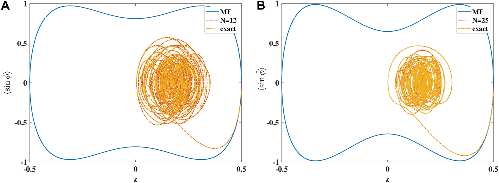
FIGURE 5. Phase-space trajectories for times up to Jt = 50 in mean-field approximation (solid blue), multi ACS (dash-dotted red), and exact quantum dynamics (dotted yellow). The initial condition is (z(0), ϕ(0)) = (0.5, 0). System parameters are as follows: (A) U/J = 1.2 and S = 20 and (B) U/J = 0.53 and S = 50.

3.5 Spontaneous symmetry breaking

So far, we have focused on the case of positive on-site interaction strength. However, it was already observed on the mean-field level that a spontaneous symmetry breaking is triggered by negative values of U beyond a certain threshold. The comparison of the mean-field with the full quantum solution and our multi-configuration ACS approach for this case will be the focus of the present section.

Because the mean-field prediction for SSB is good for large particle numbers [25], in Figure 6, we first consider the case of S = 50 and we take U/J = −0.12, leading to Λ < − 1. The results of three different levels of approximation are again displayed: mean-field, ACS with small multiplicity (here N = 10), and full quantum. In the mean-field case, displayed in panel A, we observe that the elliptic orbit for small deviations from the symmetry breaking equilibrium point (z^SSB ≈ 0.94, ϕ^SSB = 0), for larger displacements turns into a plectrum-shaped orbit around the new stable fixed point (see also panel B of Figure 1). As in the previous section, multiconfiguration ACS with a small multiplicity of N = 10 displays the spiraling away from the mean-field orbit (the “quantum effect”) in a very faithful way. The further away from z^SSB the initial condition is, the broader the range of the spiraling motion turns out to be, both in the ACS (panel B) and the exact results (panel C).

FIGURE 6

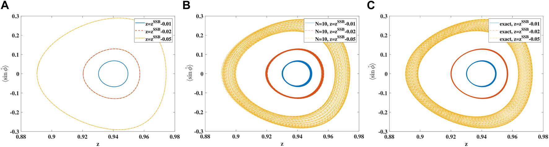
FIGURE 6. Phase-space trajectories for times up to Jt = 100 in (A) mean-field, (B) beyond mean-field with N = 10, and (C) exact quantum dynamics. Different initial conditions are displayed by different line styles: z^SSB − 0.01 (solid blue), z^SSB − 0.05 (dashed red), and z^SSB − 0.1 (dash-dotted yellow) with z^SSB = 0.94. Parameters are U/J = −0.12 and S = 50.

The case of smaller particle numbers S = 20 and U/J = −0.15 leads to z^SSB ≈ 0.71. The on-site interaction parameter lies just between the classically predicted onset of SSB and the quantum prediction. In the quantum case, it was shown that the SSB effect comes along with the switch of the amplitude from a unimodal to a bimodal distribution in a Fock-space expansion of the ground state of the Hamiltonian [45], which for large |U| becomes a so-called Schrödinger cat (NOON) state, in our notation a superposition proportional to |S, 0⟩ + |0, S⟩. For smaller particle numbers, the onset of this effect, compared to the mean-field prediction, is pushed to larger absolute values of U (i.e., stronger attractive interaction), as shown in Figure 4 of [25]. Thus, for the parameters mentioned previously, the phase-space trajectories in the beyond mean-field case show a much different behavior than in the classical case. To visualize this behavior, we have calculated the Husimi transform [42]

$Q\left(z,\varphi \right)=\langle \mathrm{\Omega }|\mathrm{\Psi }\rangle \langle \mathrm{\Psi }|\mathrm{\Omega }\rangle ,(32)$

with |Ω⟩ = |S, z, ϕ⟩. This function is localized if the time-evolved quantum state is localized around the stable fixed point, whereas it is delocalized otherwise. Taking snapshots of its dynamics for U/J = −0.15, displayed in panels A to C of Figure 7, a delocalization of the dynamics can be observed, which is very different from the mean-field prediction, which is already deep in the SSB regime. Using just two ACSs, we can thus unravel this quantum effect dynamically, without having to calculate the exact ground state. Increasing the absolute value of the onsite interaction to |U|/J = 0.19, according to Eq. 5, the new stable fixed points are moving towards larger |z| and we are choosing an initial condition with a small displacement away from the one with ϕ = 0 and a positive value of z. The beyond mean-field result (with N = 2) now also shows a restriction of the dynamics to positive values of z, i.e., it displays the phenomenon of SSB. This fact can be observed in panels D to F of Figure 7. The fact that there is no motion from right to left, when |U| is large, is due to the large energy barrier that has to be overcome in order to go from z ≈ 1, i.e., approximately the state |S, 0⟩ to z ≈ − 1, i.e., approximately the state |0, S⟩ [57].

FIGURE 7

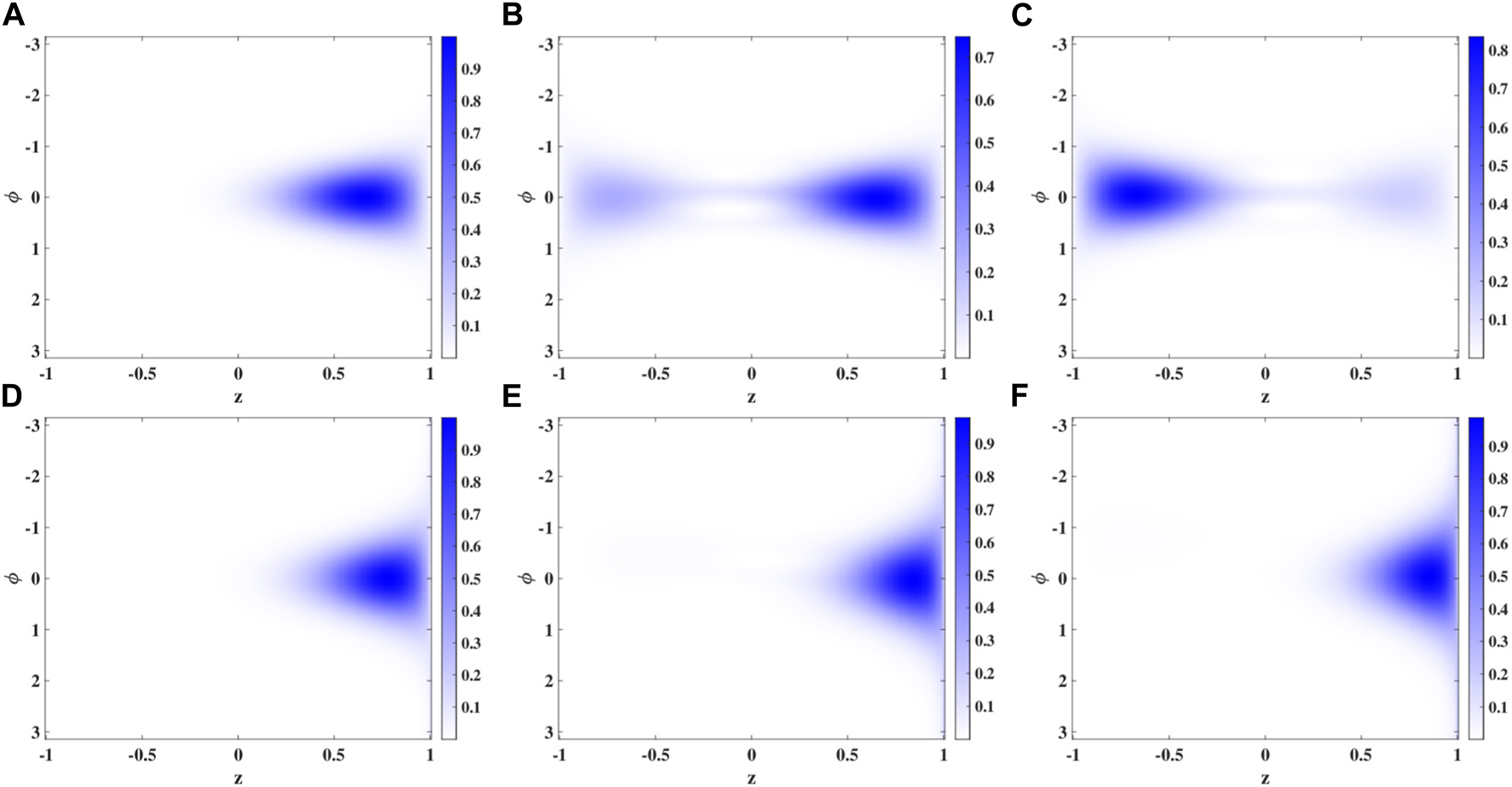
FIGURE 7. Snapshots of beyond mean-field (N = 2) Husimi distributions for S = 20 and different on-site coupling strengths and times: (A–C): U/J = −0.15 and t = 0 (A), t = 200 (B), and t = 300 (C); (D–F): U/J = −0.19 and t = 0 (D), t = 200 (E), and t = 300 (F). The initial condition for z is z^SSB − 0.05 with z^SSB = 0.71 for panels (A–C) and z^SSB = 0.83 for panels (D–F).

If one just wants to determine the transition from delocalized to localized motion beyond the mean-field prediction, it turned out that only two ACS trajectories might be enough. We will show in the remainder of this section that in order to almost faithfully predict the occurrence of the SSB transition in terms of |U| for different particle numbers, a multiplicity of N = 2 is indeed sufficient. To show this, in Figure 8, we display the onset of SSB for different values of S, as predicted by mean-field (using a single ACS), yielding the hyperbolic dependence |U|/2J = 1/(S − 1) depicted by the solid line, to the result for this onset from a multi-configurational calculation with N = 2 (red diamonds). To determine the location of the red diamonds, we have propagated the dynamics up to large enough times (Jt = 1000) to be sure that the motion is either confined to the right-hand side of phase space (i.e., z > 0) or not and have used an interval nesting strategy to determine the onset of SSB. These two results are then compared to those of the exact quantum ones (blue dots), calculated by monitoring the expansion of the ground state (GS) in terms of Fock states. If the magnitude of coefficients shows a bimodal structure and $⟨GS|S/2,S/2⟩\approx 0$, the SSB range is reached [45]. The multi-configuration ACS calculations with N = 2 show a surprisingly good agreement with the exact quantum results, even for small particle numbers.

FIGURE 8

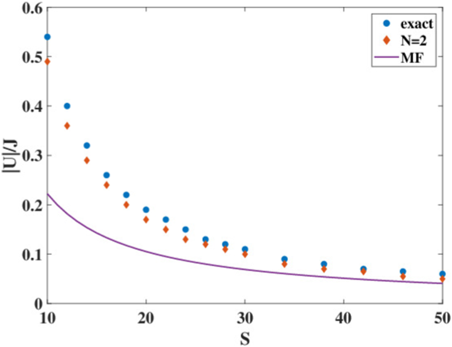
FIGURE 8. Comparison of the onset of SSB as a function of |U|/J predicted by i) ACS mean-field (solid line), ii) multi-configuration ACS with N = 2 (red diamonds), and iii) exact result (blue dots), inferred from bimodality of ground state.

4 Conclusion and outlook

We have reinvestigated some well-known physical phenomena in the dynamics of the bosonic Josephson junction model using a powerful multi-configuration technique to solve the TDSE. It was shown that, by use of an expansion of the wave-function in multiple ACSs, a decisive improvement of the classical mean-field results towards full quantum results can be achieved. Although in a Fock-space calculation, the full basis is always to be used, in the present approach, the size of the time-dependent basis function can be increased in order to achieve convergence and to reveal quantum effects. The equations of motion for the (time-dependent) variational parameters and for the expansion coefficients are derived from the time-dependent variational principle. This technical aspect of the presented work is similar in essence to the variational solution of the Gross–Pitaevskii equation with long-range interactions, based on Gaussian wave packets (Glauber coherent states) [58] as well as to the multi-configurational time-dependent Hartree–Fock method for bosons [59], although in the latter case, the employed basis functions are orthogonal. Furthermore, in contrast to the Glauber coherent states, the ACS used here conserve the particle number and are thus considered to be favorable in the present case [42]. In addition, we stress that in contrast to semiclassical methods that are based on Monte Carlo sampling of the initial conditions for mean-field trajectories and require around 10⁴ samples, here we can get satisfactory results with only a handful of variationally determined “trajectories.” The semiclassical method employed by Tomsovic et al [8] requires an order of magnitude less mean-field trajectories (even in the 6-well case) than the semiclassical initial value method used in [14], but one has to find saddle points in a complexified phase space, which is a formidable task.

The parameter space that we have covered is characterized by the strength (and the sign) of the on-site interaction, as well as by the total particle number and the initial population imbalance. First, by taking into account one additional ACS, i.e., by employing a total of just two ACSs, the beating of the population imbalance (as well as of the expectation of the sine of the phase operator) for small positive values of U can be reproduced almost quantitatively exactly, if the initial imbalance is rather small, i.e., if it is close to the classical equilibrium point at the origin of phase space. The choice of the initial phase variable of the second ACS was crucial to achieve this agreement. For larger initial imbalance, the number of ACSs needed to achieve reasonable agreement with the exact quantum results has to be increased, with more and more states needed, the higher the total particle number.

Second, our focus was on the more demanding parameter regime of MQST. Here, we could show that the use of more than 10 ACSs is necessary, if the quantum reduction compared to the mean-field value of the repulsive interaction strength at which MQST sets in is to be uncovered. As had been noticed before by Wimberger et al. [25], a single ACS is not enough to observe this effect. In the case of higher multiplicities N > 2, the choice of initial conditions for those ACS that are initially unpopulated (i., e., the ones, whose coefficients A_k in Eq. 20 are 0) was carried out by the random sampling strategy described in [48].

Lastly, for negative values of the on-site interaction and for large particle numbers, we observed a beating oscillation around the symmetry-breaking equilibrium point, which still resembles the mean-field trajectory, with the only quantum effect being the spiraling in and out of the phase-space trajectory. However, for small particle numbers, compared to the mean-field prediction, symmetry breaking only occurs for larger attractive interaction in the quantum case [25]. The fact that symmetry breaking is lost for parameters that would allow for symmetry breaking in the mean-field theory is uncovered by using just two ACSs. The new prediction of the onset of symmetry breaking in Figure 8 is very close to the exact quantum result.

In future works, the fact that the addition of only a few generalized coherent state basis functions allows for the unraveling of quantum effects can be put to good use. A possible extension of the present work would be keeping the site number at 2 but allowing for more than just a single atomic species [60]. Furthermore, driven bosonic Josephson junctions show dynamical tunneling [61], and the addition of a decay term in one of the sites allows for a characteristic modulation of self-trapping [62]. The description of these effects beyond mean-field is a worthwhile topic of future investigations. Finally, if one also allows the site number M to increase, it might be the only possibility to use flexible time-dependent GCS basis functions if numerical results showing quantum effects are asked for. This is due to the fact that the number of Fock-state basis functions increases like $\frac{(M+S-1)!}{S!(M-1)!}$ and the Fock-state-based calculations thus become unfeasible.

5 Methods

5.1 Linearized mean-field equations and their solution

From the Jacobi matrix in Eq. 12 we read off the linearized equations of motion

$\dot{z}=2J\varphi ,(33)$

$\dot{\varphi }=-\left[2J+U\left(S-1\right)\right]z(34)$

for the population imbalance and the phase difference, valid around the phase space origin. Employing the initial conditions z(0) = z₀, ϕ(0) = 0, their solution is given by

$z\left(t\right)=\frac{z_0}{2}\left[e^{2J\sqrt{-\left(1+\mathrm{\Lambda }\right)}t}+e^{-2J\sqrt{-\left(1+\mathrm{\Lambda }\right)}t}\right],(35)$

$\varphi \left(t\right)=\frac{z_0}{2}\sqrt{-\left(1+\mathrm{\Lambda }\right)}\left[e^{2J\sqrt{-\left(1+\mathrm{\Lambda }\right)}t}-e^{-2J\sqrt{-\left(1+\mathrm{\Lambda }\right)}t}\right],(36)$

with the strength parameter Λ, defined in Eq. 14 of the main text.

If Λ > − 1, we have the oscillatory solutions

$z\left(t\right)=z_0\cos \left(\mathrm{\Omega }t\right)(37)$

$\varphi \left(t\right)=-z_0\sqrt{1+\mathrm{\Lambda }}\sin \left(\mathrm{\Omega }t\right)(38)$

with the plasma frequency

$\mathrm{\Omega }=2J\sqrt{1+\mathrm{\Lambda }}.(39)$

We stress that for the specific choice of initial condition, the oscillation amplitude of ϕ depends on the strength parameter, while that of z does not.

If Λ < − 1, we obtain

$z\left(t\right)=z_0\cosh \left[2J\sqrt{-\left(1+\mathrm{\Lambda }\right)}t\right],(40)$

$\varphi \left(t\right)=z_0\sqrt{-\left(1+\mathrm{\Lambda }\right)}\sinh \left[2J\sqrt{-\left(1+\mathrm{\Lambda }\right)}t\right],(41)$

which describes a solution like the ones displayed in panel B of Figure 1, but only where the conditions |z|, |ϕ|≪ 1 are still fulfilled. Away from that regime the hyperbolic solution is unphysical.

5.2 Exact quantum calculation

For the exact quantum results, we employ an expansion of the wave-function in terms of Fock states

$|\mathrm{\Psi }\left(t\right)\rangle ={\displaystyle \sum _{i=0}^S}{b}_i\left(t\right)|F_i\rangle ,(42)$

where the sum is taken over all the states {|F_i〉} that emerge if a total of S particles is distributed over two sites. Due to the fact that one can place from zero up to S particles in, e.g., the first site, it is obvious that there are S + 1 different possibilities.

In order to completely specify the problem, the initial state has to be known, from which the b coefficients at t = 0 can be extracted. In the present work, we consider an initial state that is given in terms of a single ACS with parameters ξ₁ and ξ₂. From the definition given in Eq. 9 taken for M = 2, by applying the binomial theorem, due to ${({\widehat{a}}_i^{†})}^n|0\rangle =\sqrt{n!}|n\rangle$, we find

$\begin{array}{ccc}\hfill |\mathrm{\Psi }\left(0\right)\rangle & =\hfill & \frac{1}{\sqrt{S!}}{\left({\xi }_1{\widehat{a}}_1^{†}+{\xi }_2{\widehat{a}}_2^{†}\right)}^S|\mathrm{0,0}\rangle \hfill \\ \hfill & =\hfill & {\displaystyle \sum _{j=0}^S}\sqrt{\frac{S!}{\left(S-j\right)!j!}}{\xi }_1^{S-j}{\xi }_2^j|S-j,j\rangle ,\hfill \end{array}(43)$

which is the Fock state expansion of the initial state, providing us with the sought for coefficients at t = 0.

The first option to evolve the wave-function over time would be to solve the coupled system of linear differential equations for the b coefficients

$\mathrm{i}{\dot{b}}_j\left(t\right)={\displaystyle \sum _{i=0}^S}⟨F_j|\widehat{H}|F_i⟩b_i\left(t\right),(44)$

that follows from the TDSE, e. g., by using a Runge-Kutta method or by matrix exponentiation (which in the present case of time-independent Hamiltonian turns out to be advantageous, because the matrix exponential has to be calculated only once, before the propagation loop is started). An alternative, second option, which is also numerically exact, would require diagonalising the BH Hamiltonian [16], e.g., in the Fock basis, see also Section 2.3.1 in [63]. The time evolution is then finally given by (ℏ = 1)

$|\mathrm{\Psi }\left(t\right)\rangle ={\displaystyle \sum _{i=0}^S}{c}_i\exp \left\{-\mathrm{i}{E}_{i}t\right\}|{\mathrm{\Phi }}_i\rangle ,(45)$

where {E_i} are the eigenenergies and the {|Φ_i〉} are the eigenstates. The time-independent c-coefficients follow from the expansion of the initial wave-function in the eigenstates.

In both cases, the matrix elements of the Hamiltonian have to be set up. This does not pose a major challenge in case of small site numbers but in the general case it requires some clever way of creating and labeling of the Fock states, as described in a pedagogical way in [64].

Data availability statement

The raw data supporting the conclusion of this article will be made available by the authors, without undue reservation.

Author contributions

YQ performed the numerical studies presented in this work. Both authors contributed to the conception of the research and the writing of the article and approved the submitted version.

Acknowledgments

The authors would like to thank Prof. A. R. Kolovsky for the computer code to perform the exact Fock-space calculations (using the first option mentioned in Section 5.2), whose results are displayed here.

Conflict of interest

The authors declare that the research was conducted in the absence of any commercial or financial relationships that could be construed as a potential conflict of interest.

Publisher’s note

All claims expressed in this article are solely those of the authors and do not necessarily represent those of their affiliated organizations, or those of the publisher, the editors, and the reviewers. Any product that may be evaluated in this article, or claim that may be made by its manufacturer, is not guaranteed or endorsed by the publisher.

References

1. Greiner M, Mandel O, Esslinger T, Hänsch TW, Bloch I. Quantum phase transition from a superfluid to a Mott insulator in a gas of ultracold atoms. Nature (2002) 415:39–44. doi:10.1038/415039a

PubMed Abstract | CrossRef Full Text | Google Scholar

2. Bloch I, Dalibard J, Zwerger W. Many-body physics with ultracold gases. Rev Mod Phys (2008) 80:885–964. doi:10.1103/RevModPhys.80.885

CrossRef Full Text | Google Scholar

3. Polkovnikov A, Sengupta K, Silva A, Vengalattore M. Colloquium: Nonequilibrium dynamics of closed interacting quantum systems. Rev Mod Phys (2011) 83:863–83. doi:10.1103/RevModPhys.83.863

CrossRef Full Text | Google Scholar

4. Trotzky S, Chen Y, Flesch A, McCulloch IP, Schollwöck U, Eisert J, et al. Probing the relaxation towards equilibrium in an isolated strongly correlated one-dimensional Bose gas. Nat Phys (2012) 8:325–30. doi:10.1038/nphys2232

CrossRef Full Text | Google Scholar

5. Jaksch D, Zoller P. The cold atom Hubbard toolbox. Ann Phys (2005) 315:52–79. doi:10.1016/j.aop.2004.09.010

CrossRef Full Text | Google Scholar

6. Kolovsky AR. Bose–hubbard Hamiltonian: Quantum chaos approach. J Mod Phys B (2016) 30:1630009. doi:10.1142/s0217979216300097

CrossRef Full Text | Google Scholar

7. Milburn GJ, Corney J, Wright EM, Walls DF. Quantum dynamics of an atomic Bose-Einstein condensate in a double-well potential. Phys Rev A (1997) 55:4318–24. doi:10.1103/PhysRevA.55.4318

CrossRef Full Text | Google Scholar

8. Tomsovic S, Schlagheck P, Ullmo D, Urbina JD, Richter K. Post-Ehrenfest many-body quantum interferences in ultracold atoms far out of equilibrium. Phys Rev A (2018) 97:061606. doi:10.1103/PhysRevA.97.061606

CrossRef Full Text | Google Scholar

9. Lee C, Alexander TJ, Kivshar YS. Melting of discrete vortices via quantum fluctuations. Phys Rev Lett (2006) 97:180408. doi:10.1103/PhysRevLett.97.180408

PubMed Abstract | CrossRef Full Text | Google Scholar

10. Arwas G, Vardi A, Cohen D. Triangular Bose-Hubbard trimer as a minimal model for a superfluid circuit. Phys Rev A (2014) 89:013601. doi:10.1103/PhysRevA.89.013601

CrossRef Full Text | Google Scholar

11. Nakerst G, Haque M. Chaos in the three-site Bose-Hubbard model: Classical versus quantum. Phys Rev E (2023) 107:024210. doi:10.1103/physreve.107.024210

PubMed Abstract | CrossRef Full Text | Google Scholar

12. Nemoto K, Holmes CA, Milburn GJ, Munro WJ. Quantum dynamics of three coupled atomic Bose-Einstein condensates. Phys Rev A (2000) 63:013604. doi:10.1103/PhysRevA.63.013604

CrossRef Full Text | Google Scholar

13. Franzosi R, Penna V. Self-trapping mechanisms in the dynamics of three coupled Bose-Einstein condensates. Phys Rev A (2001) 65:013601. doi:10.1103/PhysRevA.65.013601

CrossRef Full Text | Google Scholar

14. Simon L, Strunz WT. Time-dependent semiclassics for ultracold bosons. Phys Rev A (2014) 89:052112. doi:10.1103/PhysRevA.89.052112

CrossRef Full Text | Google Scholar

15. Khripkov C, Cohen D, Vardi A. Coherence dynamics of kicked Bose-Hubbard dimers: Interferometric signatures of chaos. Phys Rev E (2013) 87:012910. doi:10.1103/PhysRevE.87.012910

PubMed Abstract | CrossRef Full Text | Google Scholar

16. Tonel AP, Links J, Foerster A. Quantum dynamics of a model for two Josephson-coupled Bose-Einstein condensates. J Phys A: Math Gen (2005) 38:1235–45. doi:10.1088/0305-4470/38/6/004

CrossRef Full Text | Google Scholar

17. Santos G, Tonel A, Foerster A, Links J. Classical and quantum dynamics of a model for atomic-molecular Bose-Einstein condensates. Phys Rev A (2006) 73:023609. doi:10.1103/PhysRevA.73.023609

CrossRef Full Text | Google Scholar

18. Javanainen J. Nonlinearity from quantum mechanics: Dynamically unstable Bose-Einstein condensate in a double-well trap. Phys Rev A (2010) 81:051602. doi:10.1103/PhysRevA.81.051602

CrossRef Full Text | Google Scholar

19. Furutani K, Tempere J, Salasnich L. Quantum effective action for the bosonic Josephson junction. Phys Rev B (2022) 105:134510. doi:10.1103/PhysRevB.105.134510

CrossRef Full Text | Google Scholar

20. Schlagheck P, Ullmo D, Lando GM, Tomsovic S. Resurgent revivals in bosonic quantum gases: A striking signature of many-body quantum interferences. Phys Rev A (2022) 106:L051302. doi:10.1103/PhysRevA.106.L051302

CrossRef Full Text | Google Scholar

21. Chuchem M, Smith-Mannschott K, Hiller M, Kottos T, Vardi A, Cohen D. Quantum dynamics in the bosonic Josephson junction. Phys Rev A (2010) 82:053617. doi:10.1103/PhysRevA.82.053617

CrossRef Full Text | Google Scholar

22. Herman MF, Kluk E. A semiclasical justification for the use of non-spreading wavepackets in dynamics calculations. Chem Phys (1984) 91:27–34. doi:10.1016/0301-0104(84)80039-7

CrossRef Full Text | Google Scholar

23. Ray S, Ostmann P, Simon L, Grossmann F, Strunz WT. Dynamics of interacting bosons using the Herman-Kluk semiclassical initial value representation. J Phys A (2016) 49:165303. doi:10.1088/1751-8113/49/16/165303

CrossRef Full Text | Google Scholar

24. Wüster S, Dabrowska-Wüster BJ, Davis MJ. Macroscopic quantum self-trapping in dynamical tunneling. Phys Rev Lett (2012) 109:080401. doi:10.1103/PhysRevLett.109.080401

PubMed Abstract | CrossRef Full Text | Google Scholar

25. Wimberger S, Manganelli G, Brollo A, Salasnich L. Finite-size effects in a bosonic Josephson junction. Phys Rev A (2021) 103:023326. doi:10.1103/PhysRevA.103.023326

CrossRef Full Text | Google Scholar

26. Albiez M, Gati R, Fölling J, Hunsmann S, Cristiani M, Oberthaler MK. Direct observation of tunneling and nonlinear self-trapping in a single bosonic Josephson junction. Phys Rev Lett (2005) 95:010402. doi:10.1103/PhysRevLett.95.010402

PubMed Abstract | CrossRef Full Text | Google Scholar

27. Leggett AJ. Bose-Einstein condensation in the alkali gases: Some fundamental concepts. Rev Mod Phys (2001) 73:307–56. doi:10.1103/RevModPhys.73.307

CrossRef Full Text | Google Scholar

28. Batchelor MT, Foerster A. Yang–baxter integrable models in experiments: From condensed matter to ultracold atoms. J Phys A: Math Theor (2016) 49:173001. doi:10.1088/1751-8113/49/17/173001

CrossRef Full Text | Google Scholar

29. Arecchi FT, Courtens E, Gilmore R, Thomas H. Atomic coherent states in quantum optics. Phys Rev A (1972) 6:2211–37. doi:10.1103/PhysRevA.6.2211

CrossRef Full Text | Google Scholar

30. Werther M, Loho Choudhury S, Grossmann F. Coherent state based solutions of the time-dependent schrödinger equation: Hierarchy of approximations to the variational principle. Int Rev Phys Chem (2021) 40:81–125. doi:10.1080/0144235x.2020.1823168

CrossRef Full Text | Google Scholar

31. Zhao Y. The hierarchy of davydov’s ansätze: From guesswork to numerically “exact” many-body wave functions. J Chem Phys (2023) 158:080901. doi:10.1063/5.0140002

PubMed Abstract | CrossRef Full Text | Google Scholar

32. Hartmann R, Werther M, Grossmann F, Strunz WT. Exact open quantum system dynamics: Optimal frequency vs time representation of bath correlations. J Chem Phys (2019) 150:234105. doi:10.1063/1.5097158

PubMed Abstract | CrossRef Full Text | Google Scholar

33. Werther M, Grossmann F. Stabilization of adiabatic population transfer by strong coupling to a phonon bath. Phys Rev A (2020) 102:063710. doi:10.1103/physreva.102.063710

CrossRef Full Text | Google Scholar

34. Fischer EW, Werther M, Bouakline F, Grossmann F, Saalfrank P. Non-Markovian vibrational relaxation dynamics at surfaces. J Chem Phys (2022) 156:214702. doi:10.1063/5.0092836

PubMed Abstract | CrossRef Full Text | Google Scholar

35. Lingua F, Richaud A, Penna V. Residual entropy and critical behavior of two interacting boson species in a double well. Entropy (2018) 20:84. doi:10.3390/e20020084

PubMed Abstract | CrossRef Full Text | Google Scholar

36. Glauber RJ. Coherent and incoherent states of the radiation field. Phys Rev (1963) 131:2766–88. doi:10.1103/PhysRev.131.2766

CrossRef Full Text | Google Scholar

37. Heller EJ. Wavepacket dynamics and quantum chaology. In: MJ Giannoni, A Voros, and J Zinn-Justin, editors. Chaos and quantum Physics. Amsterdam: Elsevier (1991). p. 547–663. Les Houches Session LII.

Google Scholar

38. Huang Z, Wang L, Wu C, Chen L, Grossmann F, Zhao Y. Polaron dynamics with off-diagonal coupling: Beyond the ehrenfest approximation. Phys Chem Chem Phys (2017) 19:1655–68. doi:10.1039/c6cp07107d

PubMed Abstract | CrossRef Full Text | Google Scholar

39. Perelomov A. Generalized coherent states and their applications. Berlin: Springer-Verlag (1986).

Google Scholar

40. Zhang WM, Feng DH, Gilmore R. Coherent states: Theory and some applications. Rev Mod Phys (1990) 62:867–927. doi:10.1103/RevModPhys.62.867

CrossRef Full Text | Google Scholar

41. Trimborn F, Witthaut D, Korsch HJ. Exact number-conserving phase-space dynamics of the m-site Bose-Hubbard model. Phys Rev A (2008) 77:043631. doi:10.1103/PhysRevA.77.043631

CrossRef Full Text | Google Scholar

42. Trimborn F, Witthaut D, Korsch HJ. Beyond mean-field dynamics of small Bose-Hubbard systems based on the number-conserving phase-space approach. Phys Rev A (2009) 79:013608. doi:10.1103/PhysRevA.79.013608

CrossRef Full Text | Google Scholar

43. Schachenmayer J, Daley AJ, Zoller P. Atomic matter-wave revivals with definite atom number in an optical lattice. Phys Rev A (2011) 83:043614. doi:10.1103/PhysRevA.83.043614

CrossRef Full Text | Google Scholar

44. Dell’Anna L. Analytical approach to the two-site Bose-Hubbard model: From Fock states to Schrödinger cat states and entanglement entropy. Phys Rev A (2012) 85:053608. doi:10.1103/physreva.85.053608

CrossRef Full Text | Google Scholar

45. Mazzarella G, Salasnich L, Parola A, Toigo F. Coherence and entanglement in the ground state of a bosonic Josephson junction: From macroscopic Schrödinger cat states to separable Fock states. Phys Rev A (2011) 83:053607. doi:10.1103/PhysRevA.83.053607

CrossRef Full Text | Google Scholar

46. Dell’Anna L. Entanglement properties and ground-state statistics of free bosons. Phys Rev A (2022) 105:032412. doi:10.1103/PhysRevA.105.032412

CrossRef Full Text | Google Scholar

47. Buonsante P, Penna V. Some remarks on the coherent-state variational approach to nonlinear boson models. J Phys A: Math Theor (2008) 41:175301. doi:10.1088/1751-8113/41/17/175301

CrossRef Full Text | Google Scholar

48. Qiao Y, Grossmann F. Exact variational dynamics of the multimode Bose-Hubbard model based on SU(m) coherent states. Phys Rev A (2021) 103:042209. doi:10.1103/PhysRevA.103.042209

CrossRef Full Text | Google Scholar

49. Smerzi A, Fantoni S, Giovanazzi S, Shenoy SR. Quantum coherent atomic tunneling between two trapped Bose-Einstein condensates. Phys Rev Lett (1997) 79:4950–3. doi:10.1103/PhysRevLett.79.4950

CrossRef Full Text | Google Scholar

50. Paraoanu GS, Kohler S, Sols F, Leggett AJ. The josephson plasmon as a bogoliubov quasiparticle. J Phys B: At Mol Opt Phys (2001) 34:4689–96. doi:10.1088/0953-4075/34/23/313

CrossRef Full Text | Google Scholar

51. Graefe EM, Korsch HJ. Semiclassical quantization of an n-particle Bose-Hubbard model. Phys Rev A (2007) 76:032116. doi:10.1103/PhysRevA.76.032116

CrossRef Full Text | Google Scholar

52. Wimberger S. Nonlinear dynamics and quantum chaos: An introduction. 2nd ed. Springer International Publishing AG (2022).

Google Scholar

53. Zibold T, Nicklas E, Gross C, Oberthaler MK. Classical bifurcation at the transition from Rabi to Josephson dynamics. Phys Rev Lett (2010) 105:204101. doi:10.1103/PhysRevLett.105.204101

PubMed Abstract | CrossRef Full Text | Google Scholar

54. Raghavan S, Smerzi A, Fantoni S, Shenoy SR. Coherent oscillations between two weakly coupled Bose-Einstein condensates: Josephson effects, π oscillations, and macroscopic quantum self-trapping. Phys Rev A (1999) 59:620–33. doi:10.1103/PhysRevA.59.620

CrossRef Full Text | Google Scholar

55. Werther M, Grossmann F. Apoptosis of moving, non-orthogonal basis functions in many-particle quantum dynamics. Phys Rev B (2020) 101:174315. doi:10.1103/physrevb.101.174315

CrossRef Full Text | Google Scholar

56. Barnett SM, Pegg DT. Phase in quantum optics. J Phys A: Math Gen (1986) 19:3849–62. doi:10.1088/0305-4470/19/18/030

CrossRef Full Text | Google Scholar

57. Zhai H. Ultracold atomic Physics. Cambridge University Press (2021). doi:10.1017/9781108595216

CrossRef Full Text | Google Scholar

58. Rau S, Main J, Wunner G. Variational methods with coupled Gaussian functions for Bose-Einstein condensates with long-range interactions. i. general concept. Phys Rev A (2010) 82:023610. doi:10.1103/physreva.82.023610

CrossRef Full Text | Google Scholar

59. Alon OE, Streltsov AI, Cederbaum LS. Multiconfigurational time-dependent Hartree method for bosons: Many-body dynamics of bosonic systems. Phys Rev A (2008) 77:033613. doi:10.1103/PhysRevA.77.033613

CrossRef Full Text | Google Scholar

60. Dufour G, Brünner T, Dittel C, Weihs G, Keil R, Buchleitner A. Many-particle interference in a two-component bosonic josephson junction: An all-optical simulation. New J Phys (2017) 19:125015. doi:10.1088/1367-2630/aa8cf7

CrossRef Full Text | Google Scholar

61. Gertjerenken B, Holthaus M. Quasiparticle tunneling in a periodically driven bosonic Josephson junction. Phys Rev A (2014) 90:053622. doi:10.1103/PhysRevA.90.053622

CrossRef Full Text | Google Scholar

62. Graefe EM, Korsch HJ, Niederle AE. Mean-field dynamics of a non-Hermitian Bose-Hubbard dimer. Phys Rev Lett (2008) 101:150408. doi:10.1103/PhysRevLett.101.150408

PubMed Abstract | CrossRef Full Text | Google Scholar

63. Grossmann F. Theoretical femtosecond Physics: Atoms and molecules in strong laser fields. 3rd ed. Springer International Publishing AG (2018).

Google Scholar

64. Zhang JM, Dong RX. Exact diagonalization: The bose–hubbard model as an example. Eur J Phys (2010) 31:591–602. doi:10.1088/0143-0807/31/3/016

CrossRef Full Text | Google Scholar