Comprehensive deep learning-based framework for automatic organs-at-risk segmentation in head-and-neck and pelvis for MR-guided radiation therapy planning

1 Introduction

Radiation therapy is one of the cornerstones of oncological treatment. In the process of radiation therapy planning (RTP), accurate definition of surrounding organs-at-risk (OARs) is essential to limit radiation dose to these areas and enable high dose delivery to the target tumor volume.

Magnetic resonance imaging (MRI) is increasingly used for cancer diagnosis and treatment as it has superior soft-tissue contrast compared to CT and can be acquired without ionizing radiation or intravenous contrast. Despite the improved image quality, manual segmentation of organs-at-risk is still a time-consuming task and often suffers from large intra- and inter-observer variability. Therefore, it is highly desired to develop an accurate and reliable method to automatically segment organs on MR images.

Within the past decade, convolutional neuronal networks (CNNs) have demonstrated spectacular results for image segmentation and accordingly, have now become the method of choice for deep-learning (DL) based automatic OARs and tumor segmentation with the prospect of shortening labor-intensive manual delineation and reducing intra- and interobserver variability [1–9]. Currently, these methods focus on one anatomical region either head and neck or the pelvic region. In contrast, we report results for both anatomies.

In the head-and-neck region, Dai et al. [1] have developed a R-CNN for automatic multi-organ segmentation for brainstem, chiasma, eyes, lenses, mandible, optic nerves, oral cavity and parotid glands. For retinoblastoma patients [2] proposed a multi-view CNN to delineate eye, sclera, vitreous, lens, retinal detachment and tumor. The authors of [3] implemented three cascaded CNNs to automatically contour parotid glands, submandibular glands, and level II and level III lymph nodes. An increased number of organs were segmented in head and neck such as in recent publications [32, 34] where an nnU-Net [37] and a full-scale attention network were used respectively. More recently, an optic nerve segmentation was published using a 3D U-Net [33].

In the pelvic region, Elguindi et al. [4] applied transfer learning using DeepLabV3+ architecture to segment multiple male pelvic structures such as bladder, rectum, urethra, rectal spacer, penile bulb, prostate and seminal vesicles. The authors in [5] addressed bladder, prostate, and rectum segmentation to support prostate radiation therapy with a deep network architecture, called STRAINet. [6] proposed a personalized auto-segmentation framework to assist online delineation of prostate, bladder, rectum, and femoral heads. The authors of [7] selected DeepMedic model including a 3D CNN and a fully connected 3D conditional random field (CRF) to segment bladder, rectum and femoral heads. Other CNN-based methods segmenting in the pelvic region focused on the delineation of one structure, such as prostate ([8] using MSD-Net) and bladder ([9] combining 2D CNN with dual pathway, adaptive shape prior and CRFs). In recent papers [35, 36], 11 and 6 organs were segmented in the pelvis region where a 3D U-Net and nnU-Net [37] were used respectively.

One of the most popular CNN architectures is the U-Net [10] and its extension, the 3D U-Net [11]. They are widely used in several publications for automatic OARs segmentation and demonstrated valuable outcomes [12–19]. [12, 13] both presented a segmentation framework that localizes and then segments 8 and 6 head-and-neck OARs, respectively. The method proposed by [12] localizes the OARs with a 3D Faster R-CNN and then segments them using an attention U-Net, while the algorithm developed by [13] utilizes standard 3D U-Nets in a cascade manner by using prior segmentations of other nearby organs (i.e., brainstem and eyes) to determine the bounding box of the next target OAR (i.e., optic nerves). [14] performs segmentation on 8 structures using an ensemble of multi-class 2D U-Nets and a graph-based postprocessing. In [15], a two-stage deep learning based-segmentation algorithm is proposed for 8 head OARs which uses 2D U-Nets-based localization followed by a 3D U-Net model to finely segment the cropped smaller area. In [16], for the automatic delineation of submandibular glands, parotid glands and level II and level III lymph nodes, a 3D U-Net was used. In the pelvic region, bladder was segmented with a U-Net-based method with progressive dilated convolution in [17]. [18] performed a large-scale study for prostatic urethra segmentation with 3D U-Net. Lastly, the authors in [19] used a 3D U-Net with focused shape modelling to delineate femoral heads.

The goal of this work is to provide AI-based tools to accelerate the organ-at-risk delineation in MR images for MR-assisted or MR-only radiation therapy planning. The main difference with respect to other publications is the MR modality (most of the AI-based OAR segmentation tools are available for CT only, while the number of MR scans used for RT planning is increasing) and large number and variety of organs in two anatomy regions (27 in head-and-neck, 10 in male pelvis—complete list of organs can be found on Figure 1) supported by our solution (as opposed to other works which focus on one or few organs). This way, the publication could serve as baseline for future publications.

FIGURE 1

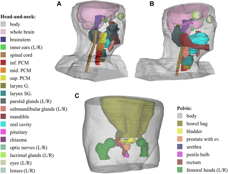
FIGURE 1. 3D illustration of manual delineation and full list of supported organs for each region. (A,B) images show the OARs in the head-and-neck region, while (C) presents the OARs in the pelvis region.—abbreviations: G.—glottic, SG.—supraglottic, PCM—pharyngeal constrictor muscle, Sup.—superior, Mid.—middle, Inf.—inferior, sv.—seminal vesicles.

The presented method uses U-Net-based deep-learning models for organ localization and segmentation (in a small sub-volume of the input) that is more efficient than segmenting large number and variety of organs (from large to small) in a large, high-resolution input image. The proposed method is also specialized to organs (or organ groups) so that it can exploit the special characteristics of the organs (symmetric, paired, large/small, partially covered). This allows us to support large number of structures and easily extend the framework with new organs.

The input of the organ contouring is a standard, high-resolution T2 scan. Using T2 images as input was motivated by the image contrast that allows confident contouring of all types of organs, furthermore this is a standard clinical image protocol (no special protocol is required) that can provide useful information for tumor as well as organ delineation.

2 Materials and methods

The presented automatic segmentation framework involved 2D and 3D deep-learning models for organ localization and segmentation, respectively. The models as well as certain pre- and postprocessing steps were specifically developed for various types of organs. The following section describes the datasets used in this work, the general segmentation framework and its variants, the applied pre- and postprocessing steps, the used localization and segmentation models, the advanced augmentations and the evaluation techniques.

2.1 Image datasets and annotation practices

The image dataset incorporated in this work is presented for the two anatomical sites: head-and-neck and pelvis. The collected dataset includes publicly available dataset (referred to as public dataset), and scans acquired inhouse or by clinical partners (referred to as private dataset).

Within the scope of this work, T2-weighted MR images were used. The rationale behind this choice is the superior image contrast (that allows confident contouring of all types of organs) and the clinical practice (standard clinical protocol, no special protocol is required).

2.1.1 Head-and-neck

For developing organ models for the head-and-neck region, a combination of public and private datasets was used. The first public dataset originated from the RTMAC (Radiation Therapy—MRI Auto-Contouring) challenge [20], referred to as AAPM dataset [21]. The AAPM dataset (available at The Cancer Imaging Archive (TCIA) website [22]) included 55 T2-weighted images of the head-and-neck region with 2 mm slice thickness and 0.5 mm in-plane pixel spacing, acquired with Siemens scanners. All scans had a reconstructed matrix size of 512 × 512 × 120 voxels and a squared 256 mm field of view (FOV). In most of the scans, the top of the head is missing, meaning that only the inferior part of the brain is visible in the scans. Therefore, another public dataset was incorporated, where the whole brain was present. This dataset is referred to as IXI dataset [23], and included 600 MR images (T1, T2 and PD-weighted, MRA, diffusion-weighted) from healthy subjects from which 31 T2-weighted exams were chosen for the development dataset for brain model training. The resolution of these scans was 256 × 256 pixels, with varying slice number (28–130) and slice thickness (1.2–5 mm). Only the whole brain was contoured in this dataset to provide more data for model training in the region above the ventricles.

Our private dataset consisted of 45 T2-weighted MR scans, all of which were acquired inhouse or by clinical partners. Out of these scans, 24 were acquired for protocol tests on healthy volunteers, and 21 scans were from cancer patients, prospectively collected for this project. They were scanned with GE MRI scanners using T2-weighted fast-recovery fast spin echo (frFSE), with 0.5–1.2 mm pixel size, 250–300 mm FOV, 240–400 mm axial coverage, and slice thickness between 1 and 3 mm.

In the development dataset 66% of subjects were cancer patients, while in the test set only cancer patients were included.

2.1.2 Pelvis

Organ models in the pelvic region were trained solely on private T2-weighted FSE image data, acquired by our clinical partners. A total of 123 exams were collected for the development and testing of the models: 17 cases were acquired on healthy volunteers (referred to as Volunteer set), the rest of the subjects were cancer patients, undergoing radiation therapy. 49 of the cancer patient scans were collected retrospectively, these scans are referred to as Prostate dataset. 57 of the scans were specifically collected for this project, these are referred to as Patient dataset. Images in the Prostate dataset were acquired with Siemens scanners and were completely uniform. All scans had 318 × 318 × 180 matrix size, 1.5 mm slice thickness and 447 mm field of view (FOV), with 180 mm axial coverage. The Volunteer dataset consisted of scans with 512 × 512 axial resolution and varying slice number (116–248), slice thickness (1–3 mm), FOV and coverage. These scans were recorded by GE scanners. The Patient dataset was also acquired by GE scanners with uniform resolution of 512 × 512 × 176 voxels, with 2 mm slice thickness, 352 mm coverage and 380 or 500 mm FOV, depending on the pixel size (0.7422 or 0.9766 mm).

In the development dataset 83% of subjects were cancer patients, while in the test set only cancer patient images were included.

2.1.3 Data annotation

Manual labelling for all datasets was performed by medical students trained and supervised by a qualified medical specialist who was experienced in clinical organ delineation. Contouring guidelines were defined based on the RTOG and DAHANCA guidelines [24] and adapted for MR-guided contouring in a consensus-based manner [25]. The structures (shown in Figure 1) included in this study are essential for RTP in the head-and-neck and pelvis regions, as irradiating them above certain dose constraints would cause severe side effects. Some organs, e.g., eyes were not fully visualized on all scans affecting the number of available manual segmentations for each structure.

From our private datasets, 10 head-and-neck and 20 pelvis cases were selected as the test dataset. The remaining cases were separated into training and validation dataset in a ratio of 4:1. For each organ the same train/validation/test separation was used for both 2D and 3D segmentation models.

2.2 Preprocessing

The segmentation framework started with a preprocessing step to achieve a pre-defined volume dimensionality, resolution, and image orientation. The steps included image standardization, and intensity normalization. For 3D models, a bounding box cut was inserted between these two steps. These preprocessing steps are detailed in the following.

2.2.1 Image standardization

Its first step was to set image orientation to Right-Anterior-Inferior (RAI) to ensure common image orientation.

For pelvis organs, slices with very low intensity (due to low signal at the boundaries of the scan) were removed from the inferior and superior part of the image, utilizing two-level Otsu threshold and morphological operations to binarize the image and generate a rough segmentation of the body. Next, the area of the body was calculated on each binarized slice, from which the median area was selected. All inferior slices with body’s area smaller than 30% of the median area and superior slices with body’s area smaller than 60% of the median area were removed. Different thresholds were used to account for different body diameter superiorly (i.e., abdomen) and inferiorly (i.e., legs) on the scan. Next, the pelvic image intensity was normalized to be between 0 and 1,000. Deharmonization (see later in Section 2.5.2) is sensitive to image intensity and it is utilized as an offline augmentation during training.

Then, the image was resampled to standard (organ-specific) voxel size. After resampling, the target matrix size was achieved by cropping or padding with zero values. The target matrix size ranged from 128 to 512. In the transverse direction, the image was cropped from the middle, however in the axial direction, the cropping is defined based on organ location (e.g., cropped from inferior part of the image in case of inferior organs). This Z direction cropping is applied for all organs except for those organs that were segmented only with 2D models, such as body, bowel bag and whole brain. Note that Z-direction cropping was applied only when the anatomy coverage is greater than 250 mm in the head or 360 mm in the pelvis scans.

2.2.2 Bounding box cut

This step was applied only in case of 3D models. For each organ, the bounding box size was pre-defined based on the training samples. The center of the bounding box was computed from the output of the 2D localizer models (see in next section) during inferencing by taking the center of mass of detected voxels. If fused 2D is an empty mask, the result of the 2D axial localizer model was utilized as base.

At the inference stage an important requirement for the bounding box was that at least 75% of it shall contain image information. This percentage was lowered to 50% in case of larynx and spinal cord, as these structures are often located near the bottom of the scan. If the requirement is not met, the bounding box was not used for training or segmentation is not provided for the case.

2.2.3 Intensity normalization

For 2D models, only a min-max intensity normalization was applied to the whole image, such that the intensity belonging to 99.9 histogram percentile was used instead of the global intensity maximum of the image.

For 3D models, the same histogram-based normalization was applied with additional mean/std normalization, but only after cutting the bounding box.

2.3 General framework and its variants

This section describes the used general framework (see in Figure 2) and its variants.

FIGURE 2

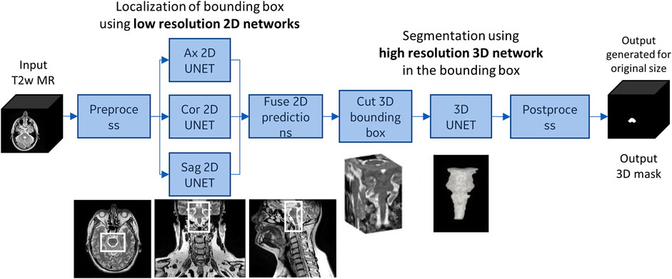
FIGURE 2. The general segmentation framework demonstrated on brainstem. First, the organ is localized with axial, sagittal and coronal 2D models, then a bounding box is cut from the 3D image based on the result of the 2D models. The 3D segmentation is applied to the bounding box only.—abbreviations: T2w—T2-weighted, Ax—Axial, Cor—Coronal, Sag—Sagittal.

2.3.1 General framework: 2D localization and 3D segmentation

Our general workflow provided a 2D segmentation for each (axial, coronal and sagittal) orientation on the low-resolution preprocessed image, then the 2D segmentations were aggregated (using majority vote). Based on the fused 2D segmentation the center of the bounding box is computed (by taking the center of mass of nonzero voxels). Using the center and the predefined organ-specific size a 3D bounding box was cut from the high-resolution image, and a 3D segmentation model was applied within the bounding box. Finally, in the postprocessing step, the result was transferred back to the geometry of the input image.

The general framework is applied for most organs in head-and-neck and pelvic regions (brainstem, chiasma, pituitary, oral cavity, spinal cord, Larynx G, Larynx SG, PCM inf, PCM mid, PCM sup, bladder, rectum, prostate, and prostate sv). In case of spinal cord, the 2D localizer models were trained to detect the superior (head-and-neck) part of spinal cord, while the 3D segmentation model was trained to return the whole spinal cord that was visible in the bounding box.

2.3.2 Variant #1—symmetric, paired organs

The first variant was used for symmetric, paired organs (inner ear, eye, lacrimal gland, lens, optic nerve, parotid gland, submandibular gland, and femoral head) with full coverage as illustrated for the parotid glands in Figure 3. This variant allows segmenting both left and right (L/R) structures using the same model. The general framework was first applied to segment the left structure. Then, the input was flipped along the X-axis and the same model was applied to segment the right structure in the L/R flipped input. Finally, the second result was flipped back with an additional postprocessing step. Both localization and segmentation models were trained using both instances of the organ (i.e., left instances and flipped version of the right instances).

FIGURE 3

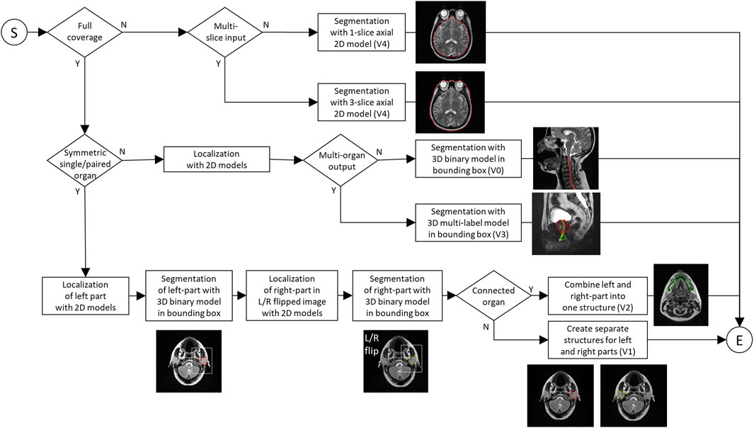
FIGURE 3. Flowchart of the segmentation involving the general framework (V0) and its variants (V1-V4). The diagram shows how the different variants are applied based on the characteristics of the organs to be segmented.

In special cases, small organs such as lens and lacrimal gland is detected in combination with a larger organ. In this case the localization models were trained to detect the union of one or more small organs and a larger guiding structure. The 3D segmentation was then performed within the combined bounding box.

2.3.3 Variant #2—large, symmetric single organ

The second variant was used for mandible, which is a large, symmetric, single organ with full coverage. This variant was based on the same principles as the first one except for three differences. First, the organ was cut into L/R parts for model training. Second, the 3D segmentation model was trained to return all of the organ that was visible in the bounding box (i.e., in addition to the whole left part, the visible section of the right part was also segmented). Third, the left and right parts were combined into a final segmentation.

2.3.4 Variant #3—multi-label segmentation

The third variant was used for small, connected organs as illustrated in Figure 3 for the prostate, the urethra and the penile bulb. In this case the localization models were trained to detect the union of the organs, while the 3D segmentation model was trained to return multiple structures (i.e., multi-label segmentation). With such method, small organs such as urethra and penile bulb can be well-localized and segmented in connection with a larger structure (prostate).

2.3.5 Variant #4—large, single organ with partial coverage

The last variant (shown in Figure 3) was used for large, single organs with partial coverage such as brain, body, and bowel bag which cannot be segmented with 3D model due to their large size and varying coverage. In this case single- or multi-slice 2D axial model was trained to segment the organ in each slice separately. These models produce one output mask for each slice, where the multi-slice model requires 3 consecutive input slices (i.e., previous, actual, next).

2.4 Localization and segmentation models

The localization of the organs, i.e., finding the center of the 3D bounding box, was based on 2D models which segment the organ on axial, coronal, and sagittal slices. This (coarse) segmentation was performed using 2D U-Net trained for axial, coronal, and sagittal slices, separately. Some structures (e.g., brain, head body, pelvis body, bowel bag) were segmented using 2D axial model only, while most of the structures were segmented with 3D model within the localized bounding-box.

The models were trained on an NVIDIA V100 GPU, with 16 GB of memory.

2.4.1 2D U-Net

The 2D model’s architecture (shown in Figure 4) was a state-of-the-art U-Net [10] with transposed convolution (instead of upsampling layer), batch normalization and dropout. The input size varied among organs (in the range of 128–512), but the default was a 128 × 128 single-channel mask representing one slice of the MR image. For bowel bag and head-and-neck and pelvis body, the input was a 512 × 512 × 3 multi-channel matrix representing 3 consecutive slices of the MR image. The output was a single-channel matrix.

FIGURE 4

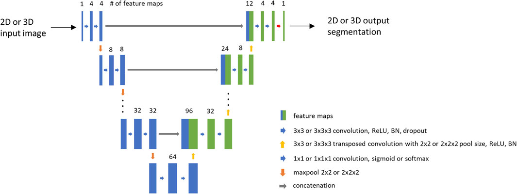
FIGURE 4. Base architecture of the U-Nets. The number of feature maps is displayed based on the whole brain model. For multi-slice models, the input image has 3 slices. For multi-label models, the output label number varies.

The 2D model training was performed using a balanced set of positive and negative image slices, except for pelvis body, where no negative slice was used. A slice was considered positive if it contains the organ of interest.

During the model training, Adam optimizer was used with 0.001 initial learning rate which was halved after the validation loss has not decreased in 5 epochs. Batch size was set to 16. The training and validation loss was calculated based on Dice similarity coefficient (DSC). Initial filter number was set to 4 for head-and-neck and pelvis body and whole brain and 16 for other models. The number of epochs ranged from 30 to 75, the patience for early stopping ranged from 10 to 30. The number of pooling layers was set based on target matrix size, ranged from 4–6 for 128–512 matrix size.

Offline and online augmentations were applied to the training data during training. The set of applied augmentations varied organ by organ based on their characteristics.

The offline augmentations include organ elongation, left-right flip, and deharmonization (c.f. Section 2.5.2). In case of paired organs (e.g., eye), the left-right flip augmentation was used to generate additional training sample for the left part using the flipped image and the flipped version of the right part.

As an online augmentation, the preprocessed image was randomly cropped to the target size (to simulate varying scan coverage). Signal intensity augmentation was also applied using the following function: $f\left(x\right)=m*x+b$, where (by default) $\left.m\in [\mathrm{0.6,1.0}\right)$ and $\left.b\in [-\mathrm{0.1,0.1}\right)$ except for chiasma, where $\left.m\in [\mathrm{0.5,1.0}\right)$ and $b=0$. Additionally, Gauss noise (only for head-and-neck organs), 2D shift, 2D zoom and bias augmentation (for pelvis organs) was applied to some organs.

2.4.2 3D U-Net

The 3D model’s architecture (shown in Figure 4) was derived from the 2D model’s architecture such that the 2D layers were replaced with 3D layers (convolution, pooling, transposed convolution), and dropout was not utilized in the 3D network. The output of the network was a 3D probability mask. In case of some organs (urethra, penile bulb), multi-channel output was generated, where different output channels represented the different structures.

The 3D model was used to segment the organ at fine resolution inside the bounding box. The input size was organ specific. During 3D model training the center of the bounding box was shifted randomly before cutting (as additional augmentation step) to account for possible inaccuracies in the localization.

All single-label models were trained for 100 epochs except for lens and lacrimal where epochs were set to 150. The batch size was set to 6 (due to GPU memory limitations). The used optimizer was Adam with 0.001 initial learning rate. Based on the validation loss early stopping was applied with a patience of 30 epochs. The training and validation loss was standard DSC for the single-label and MCUSM (short for Multi Class Union Smoothed Minimum) DSC for multi-label models (described in Section 2.4.2.1).

Offline and online augmentations were also applied during 3D model training. Offline augmentations included organ elongation, L/R flip, and deharmonization. During model training, intensity augmentation was utilized based on a simple multiplication with number chosen randomly between 0.5 and 1.0. In case of 3D brainstem model training, the local variation of intensity was simulated in a few randomly selected, consecutive slices (based on observations of patient scans). Additionally, Gauss noise (only for head-and-neck organs), 3D shift, 3D zoom and bias augmentations (for pelvis organs) were applied.

2.4.2.1 MCUSM DSC loss

For multi-label model training, a new DSC score-based loss was developed which shifts the focus of the model to the more difficult (usually smaller) organs, thus enabling proper segmentation of difficult small organs located next to a large one.

The MCUSM DSC loss was calculated as follows:

1. DSC score was calculated for each but background channel:

$dic{e}_i=2*\frac{\left|X_i\cap Y_i\right|+\epsilon }{\left|X_i\right|+\left|Y_i\right|+\epsilon },wherei=1,\dots N$

where $\left|X\right|$ and $\left|Y\right|$ are the number of voxels in the automatic and manual segmentations, respectively, $\left|X\cap Y\right|$ was the number of overlapping voxels between the two segmentations and $N$ represents the number of channels.

2. Then, the channel-wise DSC was summed up by:

$dic{e}_{sum}=-\frac{1}{\beta }\log \left({\sum }_i-e^{\beta dic{e}_i}\right),$

where β was experimentally determined to ensure satisfactory convergence for the difficult labels, in our case $\beta =4$.

3. Additionally, a $dic{e}_{union}$ was calculated, where we take the union of all channels (except the background channel) and compute DSC score against the union ground truth labels. This allows balancing the segmentation errors differently between the parts of the union versus outside the union (i.e., background).

4. The last step was to sum up the DSC:

$loss=-\left(\alpha |*||d|i|c|e_{sum}|+|\left(1-\alpha \right)|*||d|i|c|e_{union}\right)$

where $\alpha =0.7$.

2.5 Advanced augmentations

2.5.1 Elongate organs

The elongation method (shown in Figure 5) was applied to those organs which are anatomically separated but there was no clear boundary between them (such as spinal cord and brainstem, optic nerves and chiasma, parts of PCM). The method was used to incorporate parts of the other structure with a predefined length and only utilized for model training to provide segmentation without gap between the two structures.

FIGURE 5

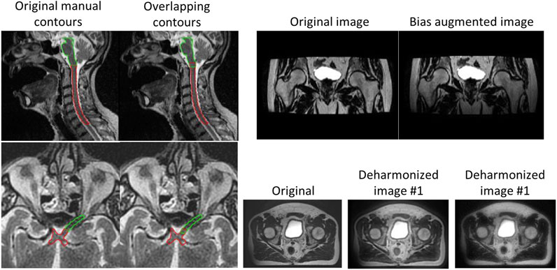
FIGURE 5. Advanced augmentations. Left: organ elongation to ensure there is no gap between connected organs (brainstem/spinal cord and optic nerve/chiasma); Right: bias augmentation (top), deharmonization (bottom).

2.5.2 Deharmonization

The motivation of data deharmonization was to change an input image to mimic various styles or appearances of MR images from the unseen world. Basically, it decomposed a given image into different images belonging to different spatial frequency bands and changed statistics such as mean and standard deviations of each band image and combined the modified band image into an image with a different appearance.

$L_0\left(x\right)=I\left(x\right)$

$L_i\left(x\right)=L_{i-1}\left(x\right)*G\left(x;{\sigma }_i\right)$

$I_i\left(x\right)=L_{i-1}\left(x\right)-L_i\left(x\right)fori=1,\dots ,B-1$

$I_B\left(x\right)=L_{B-1}\left(x\right)fori=B$

The input image ($I\left(x\right)$) was decomposed into $B$ bands $I_i\left(x\right)$ using the equations above, where $G\left(x;{\sigma }_i\right)$ was Gaussian smoothing and ${\sigma }_i$ was the Gaussian sigma. After decomposing, the intensity from each band was randomly modified by changing the mean and standard deviation with linear scaling and translation operations. Then, the changed energy band images were combined using sum operation. The randomly chosen mean and standard deviation were bounded by the statistical range obtained from reference images.

Two examples for deharmonized image are presented in Figure 5.

2.5.3 Bias augmentation

In some clinical MR images (scanned with 3D protocol) significant intensity darkening can be observed in the most inferior slices. To simulate this typical artifact seen on T2-weighted MR scans, bias inhomogeneity augmentation was implemented using a T2-weighted MR specific intensity non-uniformity (INU) field published by BrainWeb [26–30]. The INU field was estimated from real MRI scans, as a non-linear, slowly varying field of a complex shape. Non-linear scaling was applied to the field with an exponent chosen randomly from a predefined range, so each time it was applied, the scans were darkened with different intensities. An example is shown in Figure 5.

2.6 Postprocessing

2.6.1 Organ-specific steps

The model prediction was transformed back to original resolution and binarized using 0.5 as threshold. In case of multi-label output, the binarization was performed for each channel. In the next step, largest (3D) connected component search was performed on the binary mask(s). For some organs (mandible, optic nerve, and spinal cord) all components which were greater than a pre-defined percent of the total volume was kept (in addition to the largest one). Additional organ-specific steps were applied to most organs such as 2D or 3D hole filling, 2D morphological closing or 2D dilation operation in axial plane with kernel size of 3 × 3. Finally, the orientation was set back to original image orientation to ensure alignment with the input MR scan. Anatomically incorrect overlaps between neighboring organs were resolved by either assigning voxels to the closest organ, or prioritizing structures over another (e.g., pituitary over brain).

2.7 Evaluation

The accuracy of the organ segmentation models was evaluated on the private test cases in quantitative and qualitative ways. One possible way to evaluate an MR-based organ auto-contour is to compare it with CT-based manual- or auto-contour after registration. However, in such case the registration can introduce small contour mismatch that is measured as segmentation error. Furthermore, some of the organs are more visible in MR which allows more precise definition of the ground-truth. In an MR-only workflow, where synthetic CT is generated from MR scan, there is no CT available. In this work the evaluation was based on the T2-weighted MR image without incorporating other (MR or CT) scans.

The following subsections describe the two evaluation methods.

2.7.1 Qualitative evaluation

For each anatomical site, radiation oncologists from two independent institutions reviewed the contours and evaluated them using Likert scores.

The Likert score was defined to reflect the clinical usability of the auto-contour as presented later. This scoring provides more information compared to the binary (acceptable/unacceptable) classification, where small differences can get lost in the reviewing process. The Likert scores were defined as follows:

• Score 1: clinically unacceptable contour requiring complete recontouring (e.g., due to wrong organ localization or severe under- or over-segmentation)—considered as failed segmentation.

• Score 2: clinically unacceptable contour requiring significant correction and/or recontouring (e.g., on several slices, which would take long time)—considered as failed segmentation.

• Score 3: clinically unacceptable contour that can be used for radiation treatment after some correction, which requires significantly less time than recontouring—considered as successful segmentation as it has clinical value.

• Score 4: clinically acceptable contour with minor, optional corrections. This option was introduced to handle inter-operator variability and individual preferences.

• Score 5: clinically acceptable contours, no modifications required.

• Additionally, a contour was rated N/A when the organ was not considered relevant from radiation therapy’s point of view. This rating covers scenarios when the contour accuracy cannot be assessed (due to insufficient image quality, incomplete organ coverage) or the contour was not considered OAR (tumor infiltration, artificial eye lens).

2.7.2 Quantitative evaluation

The auto-segmentation results were evaluated using common quantitative metrics that are widely used in the medical image segmentation domain: DSC, precision, recall, and Surface DSC scores.

The Dice similarity coefficient (DSC) is a metric used to calculate the volumetric overlap of two datasets: in this case, it directly compares a segmentation generated by the deep-learning model against the ground-truth manual contours.

Precision demonstrates the accuracy of the identified positive pixels (minimizing false positives), while recall targets the ability to capture most of the actual positive pixels of the target organ (minimizing false negatives). These values are often used to characterize over- or under-segmentation.

The assessment of how well the surface of the auto-contour is aligned with that of the manual contour provides another useful piece of information about the segmentation accuracy, this information can be obtained using the Surface DSC metric. The Surface DSC measures deviations in border placement by computing the closest distances between all surface points of the auto segmentation relative to the surface points of the manual reference contour [31]. Its value indicates a percentage of the surface points that lie within a defined tolerance.

2.8 Ethical statement

The MR scans used in this work for model training or evaluation involve public datasets, internal volunteer scans, clinical volunteer and patient scans which were collected with the consent of the subjects. The head-and-neck patients were participants in a study that was reviewed and approved by the Medical Ethics committee of Erasmus Medical Center (Deep MR Only, MEC 19-0805). For head-and-neck volunteer cases, the number of the ethical protocol at Erasmus Medical Center is 2014-096. For pelvis volunteer data, the study was approved by the Faculty of Medical Sciences Research Ethics Committee, part of Newcastle University’s Research Ethics Committee (ethical approval: 1878/873). For the pelvis patient cases acquired by Siemens scanners, the radiotherapy consent included consent for patient data to be used for research purposes and the retrospective use of the anonymized data for this research project was approved by Newcastle upon Tyne Hospitals NHS Foundation Trust. For the remaining pelvis patient cases, HRA and Health and Care Research Wales has approved the study with IRAS project ID 265421.

3 Results

Table 1 shows the average DSC, precision, recall, and Surface DSC (using 1 and 2 mm tolerance) accuracy and the Likert scores assigned by the two institutes for each organ. In general, it was observed that high DSC scores were aligned with high clinical scores, but there were a few exceptions observed among the models that is discussed in more details.

TABLE 1

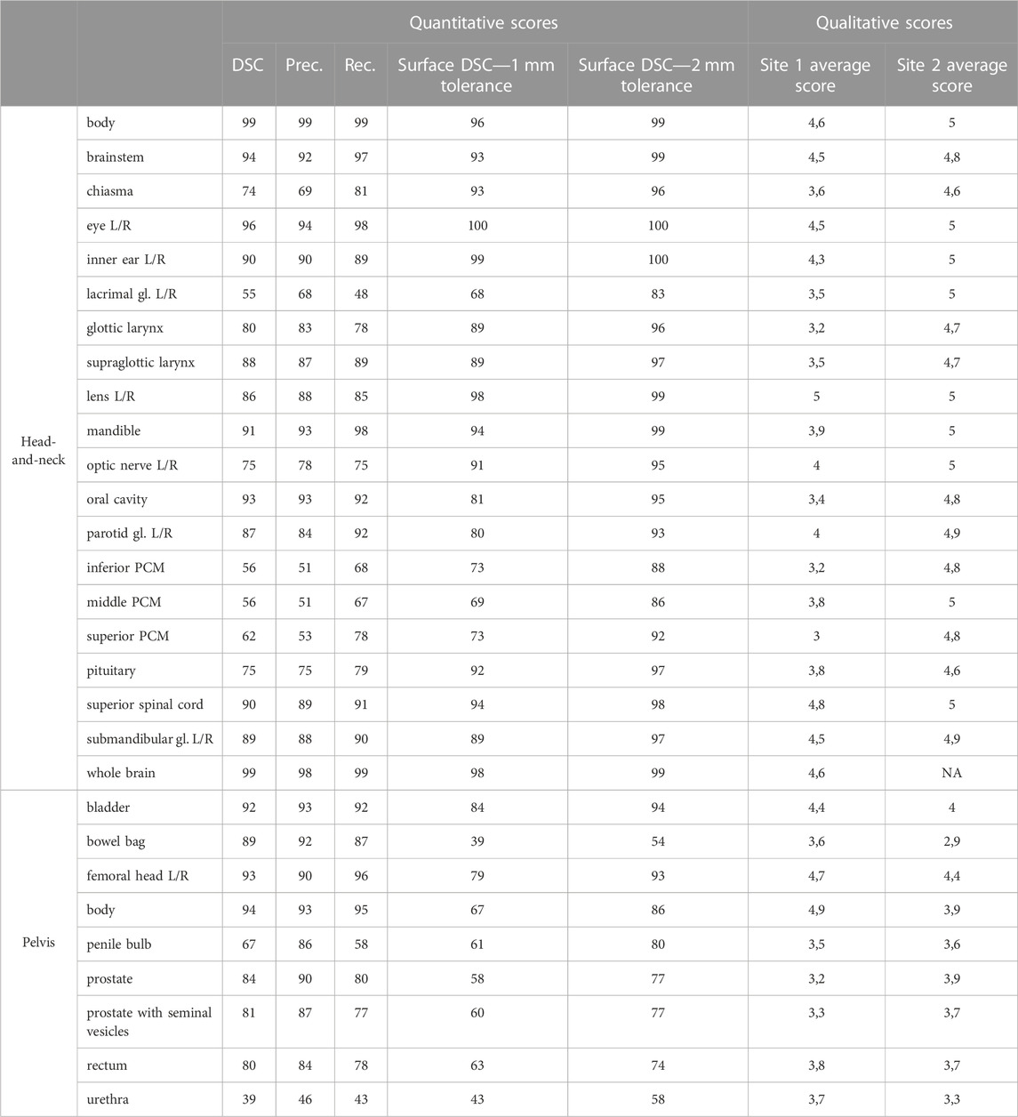
TABLE 1. The results of the quantitative and qualitative evaluation. Left and right parts of organs are averaged. Qualitative scores are given in percentage. (Prec.—precision; Rec.—recall).

There was also some difference observed in the Likert scores assigned by the different clinical sites. Although, there was a consensus regarding the definition of organs contours, there was no synchronization between the sites about the exact understanding of the Likert scores, which can be an explanation for the different interpretation.

3.1 Head-and-neck OARs

In the head-and-neck region, the best average DSC (above 99%) belongs to body and whole brain, which are large structures. The eye, the brainstem, the oral cavity, the mandible, the spinal cord, and the inner ear, which have very clear boundaries in T2w MR scans, demonstrated high accuracy (>90%). The submandibular glands, the supraglottic larynx, the parotid glands, which are medium sized organs, achieved good accuracy (85%–90%). The lens, the glottic larynx, the pituitary gland, the optic nerves, and the chiasma, which are small or thin organs (where a few voxel difference can cause significant decrease in DSC), show moderate accuracy (70%–90%). The worst DSC (55%–65%) were achieved by the different parts of the PCM and the lacrimal glands which are challenging to delineate on T2-weighted images.

The last 2 columns of Table 1 show the average scores assigned by 2 clinical sites for each organ. The head-and-neck cases were reviewed by one clinician in both sites. Site 2 did not rate the whole brain because the organ was not fully covered by the MR scans. According to the average scores assigned by Site 1, lens, spinal cord, body, whole brain, eye, brainstem, inner ear showed the best accuracy (>4). Moderate average score (3.7-4) was assigned to parotid gland, optic nerve, mandible, pituitary, and middle PCM, while the lowest scores (3-3.6) were assigned to chiasma, supraglottic larynx, lacrimal gland, oral cavity, glottic larynx, and inferior PCM, and superior PCM. The average Likert scores were in good agreement with average DSC scores for most of the organs, but there were a few outliers. Lens (5 vs. 86%), middle PCM (3.8 vs. 56%), lacrimal gland (3.5 vs. 55%) were rated better, while mandible (3.9 vs. 91%), supraglottic larynx (3.5 vs. 88%), glottic larynx (3.2 vs. 80%), and oral cavity (3.4 vs. 93%) were rated lower than one would expect from the DSC accuracy.

According to Table 1, Site 2 assigned different scores to the head-and-neck organ contours. In general, they rated all structures better (average of all scores 4.87) than Site 1 (average of all scores 3.99).

The average DSC was higher than 85% for 12 head OARs. For almost all of them, also the Surface DSC metrics were high: above 88% for 1 mm tolerance and above 95% for 2 mm tolerance. The only exception was the parotid gland where the Surface DSC was 80% for 1 mm tolerance and 93% for 2 mm tolerance.

There were few outliers among high DSC results. Despite the 88% DSC, and 89% Surface DSC (with 1 mm tolerance) and 96% (with 2 mm tolerance), the supraglottic larynx achieved low average score of 3.5 from Reviewer 1. Similarly, mandible was rated as only 3.9 by Reviewer 1 although its model performance was 91% of the DSC, 94% of the Surface DSC with 1 mm tolerance and 99% with 2 mm tolerance. Finally, oral cavity got a Reviewer 1’s score of only 3.4 while reaching 93% of the DSC. However, its Surface DSC values were lower (81% and 95% respectively).

There were 8 head models with performance lower than 80% DSC. Seven of them were rated between 3 and 4 by Reviewer 1. The only outlier from this group was optic nerve model which had an average clinicians’ score of 4.5 with an average DSC of 75%. It is noticeable that its Surface DSC values were high (91% and 95%). The optic nerve is a very small and thin structure, so it is very vulnerable to even small mismatches between the ground truth and auto-segmentation which is reflected in the DSC. It can explain why it was rated higher by clinicians despite the low DSC value.

There were a few lower-rated models with moderate DSC performance that still had higher Surface DSC. Such examples are: glottic larynx (80% of the DSC, 89% of the Surface DSC with 1 mm tolerance and 96% with 2 mm tolerance), chiasma (74% of the DSC, while 93% and 96% of the Surface DSC respectively), pituitary (75% of the DSC, while 92% and 97% of the Surface DSC respectively). The size (or diameter) of these organs is very small, so small deviations of the contour may result in significant decrease of volumetric DSC.

3.2 Pelvis OARs

In the pelvis region the highest DSC accuracy (>90%) was achieved by the body, the femoral head, and the bladder models which are large structures with well-defined boundaries. Bowel bag, prostate, prostate with seminal vesicles, and rectum, which are very heterogeneous structures, showed moderate accuracy (80%–90%). The worst accuracy (70%>) was achieved for the penile bulb and urethra. Due to the large scan coverage (used for pelvis scans) the top and bottom slices were usually affected by signal loss or imaging artifacts (e.g., wrap around). These circumstances affected the most the accuracy of the body, the bowel bag, the rectum, the penile bulb, and the urethra in the superior and inferior part of the image.

According to the scores of Sites 1 the body, the femoral heads and bladder were the most accurate contours, which was also reflected by the highest Likert scores (>4). The rectum, urethra, bowel bag, and penile bulb had moderate average score (3.5-4), while the prostate (w/o seminal vesicles) were rated the worst by the clinician. The largest discrepancy between qualitative and quantitative scores was observed for urethra (3.7 vs. 37%) bowel bag (3.6 vs. 89%) and prostate (3.2 vs. 84%). The urethra is a thin structure where some voxel difference from ground-truth can result significant decrease of DSC score. In contrast, the bowel bag is a large structure that may require significant manual adjustments even if the DSC score is relatively high. The prostate is a special structure in the sense that it is often also the treatment target (not organ-at-risk) which requires very precise delineation, so small inaccuracy can result in lower score.

There were some differences between the Likert scores assigned by the 2 sites to the pelvic structures. The average of all scores was very close (3.9 for Site 1 and 3.7 for Site 2), but there were significant differences in case of a few structures. The body and bowel bag were rated better in Site 1 (4.9, 3.6) than in Site 2 (3.9, 2.9) because Site 2 was more critical with segmentation inaccuracies in the top and bottom slices of the input scans, while Site 1 considered the contours on those slices less relevant. There was also large difference between the scores of the prostate that was better rated by Site 2 (3.9 vs. 3.2).

Three pelvis models (bladder, femoral head, and body) reached the average DSC above 90% which was in alignment with clinicians’ average scores that varied from 4.2 to 4.5. Except for the body, these organs had the highest values of the Surface DSC with 1 mm tolerance (79%–84%) as well as with 2 mm tolerance (93%–94%). In case of the body, the Surface DSC values are much lower (67% and 86% respectively). This is a common observation for pelvis organ auto-segmentation generated by 2D deep learning models. Due to the 2D approach the body and the bowel bag were segmented at the topmost slices of the pelvis scan, which are affected by various artefacts (respiratory, wrap-around) causing the model to perform suboptimal. These organs are larger compared to others, therefore low Surface DSC results suggest that there was a systematic under- or over-segmentation; however, the average clinicians’ score for the body shows that this error does not affect the auto-segmentation too significantly, as it usually requires either none or only minor correction.

For the remaining six pelvis organs, there was no clear correlation between quantitative and qualitative metrics. Urethra and penile bulb had the lowest evaluation metric results (DSC of 39% and 67%, Surface DSC with 1 mm tolerance of 43% and 61% and with 2 mm tolerance of 58% and 80% respectively) and were rated with average of 3.5 and 3.6 by clinicians. The urethra is a thin organ, so a visually good segmentation may have small overlap (i.e., DSC) with the ground-truth. The penile bulb is also a small structure (visible on few slices only) accordingly small inaccuracies translate in low DSC value. Organs like prostate, rectum, and bowel bag had higher DSC (80%–89%), but their Likert scores were relatively low (3.2–3.7). It is remarkable though that their Surface DSC values were substantially lower than better-rated organs, which indicates need for more adjustments. It highlights the importance of taking into consideration both DSC and Surface DSC metrics when evaluating medical auto-segmentations.

3.3 Common segmentation errors

Table 2 demonstrates the common segmentation errors observed during the qualitative evaluation. An error was considered common, when it was observed in more than half of the reviewed contours. Those head-and-neck organs which are not listed in the table, had no common segmentation errors reported by the reviewers.

TABLE 2

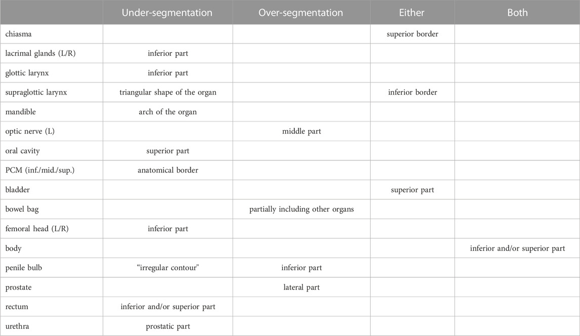
TABLE 2. Common segmentation errors observed during qualitative evaluation.

A typical error of the 3D segmentation model was the inaccurate detection of the non-visible boundaries which are found at the edge of continuous anatomy structures (e.g., brainstem/spinal cord, PCM inf./mid./sup., larynx glottic/supraglottic). These boundaries are defined by nearby anatomy landmarks, such as the odontoid process for brainstem, or the arytenoid cartilages, the hyoid bone, and the second cervical vertebrae for PCM and larynx. In such cases the connected structures are typically correctly segmented, but the boundary between the connected parts was not found at the expected axial slice because there was no visible boundary that could have been learned by the 3D segmentation model.

Another common error was the inaccuracy at the top- or the bottom-most slice of the organ, especially where the structure boundary is defined by a straight plane (e.g., bottom of the femoral heads). This is also a consequence of using 3D model that results in a smooth 3D contour with small deviations. These deviations become apparent when the result is evaluated in 2D axial slices in form of smaller fragmented islands which were typically considered false positive by the clinicians. Organ specific segmentation errors are displayed on Figure 6; Figure 7.

FIGURE 6

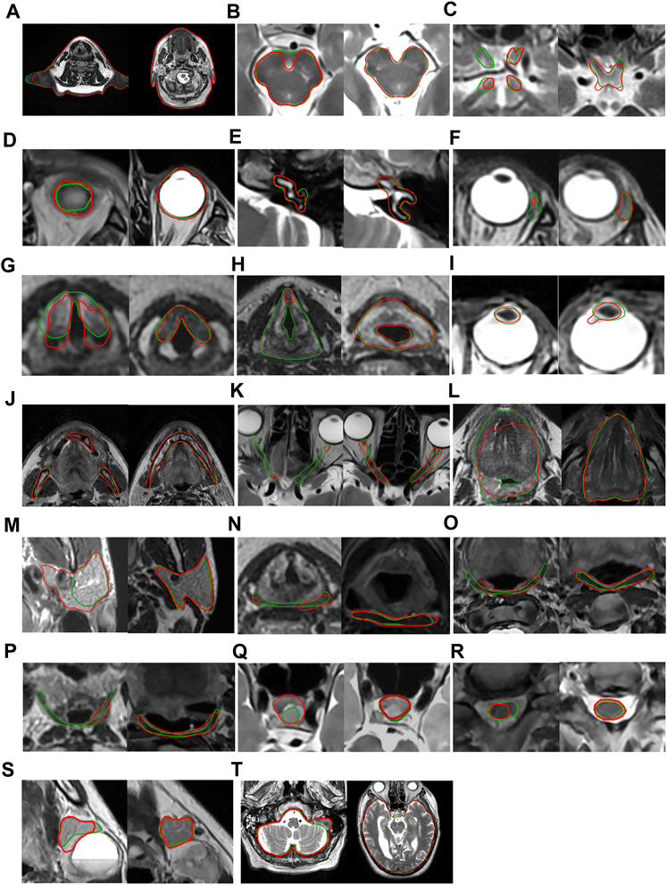
FIGURE 6. Worst (left) and best (right) results in head-and-neck based on qualitative score (green—manual segmentation, red—auto-segmentation)—from left to right and top to bottom: (A) head body, (B) brainstem, (C) chiasma, (D) eye, (E) inner ear, (F) lacrimal gland, (G) glottic larynx, (H) supraglottic larynx, (I) lens, (J) mandible, (K) optic nerve, (L) oral cavity, (M) parotid gland, (N) inferior PCM, (O) middle PC, (P) superior PCM, (Q) pituitary, (R) superior spinal cord, (S) submandibular gland, (T) whole brain.

FIGURE 7

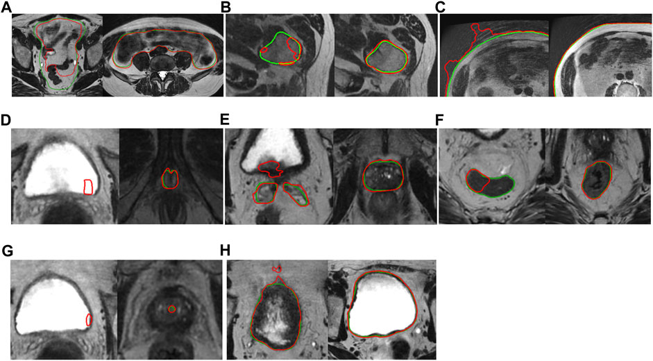
FIGURE 7. Worst (left) and best (right) results in male pelvis (green—manual segmentation, red—auto-segmentation)—from left to right and top to bottom: (A) bowel bag, (B) femoral head, (C) pelvis body, (D) penile bulb, (E) prostate and seminal vesicles, (F) rectum, (G) urethra, (H) bladder.

4 Discussion

This work presents a comprehensive DL-based framework for OAR localization and segmentation for MR-based radiation therapy. The proposed method was evaluated for head-and-neck and pelvic anatomy in both qualitative and quantitative ways. According to the qualitative evaluation of the head-and-neck segmentation, the clinician from Site 1 found 72% of the auto-contours acceptable with no or minor corrections, and Site 2 scored all contours acceptable. The qualitative evaluation of the pelvis segmentation showed that both sites found similar percentage of the organ contours clinically acceptable (73% and 69%). These results indicate that the presented method could make impact to the clinical workflow of MR-based radiation therapy planning, following further evaluation in larger and more heterogeneous patient cohorts.

To enable comparison with the prior-art, the auto-contours were compared with ground-truth using standard quantitative measures. Table 3; Table 4 show the comparison between DSC scores obtained by the proposed method and the current state-of-the-arts for head-and-neck and pelvis organs, respectively. The best accuracy for each organ is highlighted with bold font style. As one can see in Table 3, 7 out of 20 head-and-neck organ models produced the best results compared to the reported state-of-the-art. Additionally, the eye model’s performance was just slightly worse (only 1% difference) compared to the best state-of-the-art DSC. The remaining organs’ model either performed in the mid-range of the collected DSC scores (for 5 out of 20 organs) or have not been targeted by other MR-only studies (for 7 out of 20).

TABLE 3

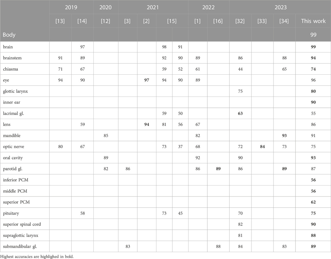
TABLE 3. DSC (%) comparison of the proposed and prior-art methods for head-and-neck OARS. The accuracy of the proposed method was reported on a different dataset compared to the literature.

TABLE 4

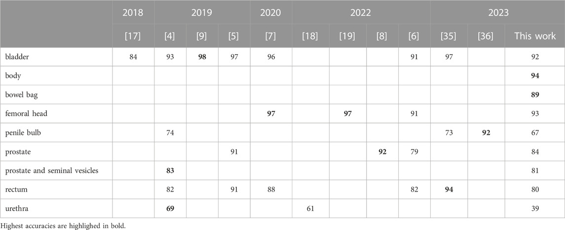
TABLE 4. DSC (%) comparison of the proposed and state-of-the-art methods for male pelvis OARs. The accuracy of the proposed method was reported on a different dataset compared to the literature.

According to Table 4 the pelvis segmentation performance was lower than head-and-neck as none of them resulted in best outcome compared to the prior-art. For pelvis body and bowel bag, based on our extensive literature review, studies have not yet reported any results so far. Three of the 9 organ models were in the middle range of the prior art. The DSC accuracy of the union of prostate and seminal vesicles was reported by only one publication which provided results close to ours. The remaining models’ performance was below currently reported state-of-the-art results. This can be due to the fact that the input scan of this study has larger (40–50 cm) FOV which allows less precise segmentation due to lower resolution.

Regarding the comparison with the prior art, it is important to mention that majority of the published methods were designed for segmenting one or just a few organs. Furthermore, the MR modality shows more variation in image quality (compared to the more standardized CT), which makes it challenging to compare different works. The definition of organs may also vary across publications. For example, femoral head may involve only the spherical part, but the proposed method segments significant part of the bone.

The mean inference time of the segmentation framework (including all organs) was about 21 min for a head-and-neck, and 6 min for pelvis using a normal GPU. Although, there is a plan to further optimize the workflow in the future, it would still accelerate the labor-intensive delineation process in RTP that can take several hours for one case.

The segmentation pipeline is implemented in an end-to-end way in a sense that the input is the MR scan and the output is the set of segmented organ contours. If an error occurs during the segmentation of a structure (localization fails or segmentation returns empty mask) no output is generated for the given structure which does not affect the segmentation of other structures. However, while we recognize that multi-task models are the future of deep-learning-based segmentation, today some practical limitations still hold us back from training and inferencing such large models. With the currently-available GPU tools it is challenging to train large, multi-task models which take a high-resolution 3-dimensional scan as input and segment large number and variety of structures (large-small, round-flat, thin-thick) with good accuracy. From AI model maintenance’s point of view, it is more efficient to develop models which segment only one or just a few structures. This way there is no need to retrain a large model when the accuracy of a few organs shall be improved, while others are up to standard.

One limitation of this work is that the organs with tumorous growth and healthy organs were not separately evaluated, which impacted both the model performance (due to distorted organ boundary) and the given qualitative scores (as target needs to be highly precisely contoured). The other limitation is that the evaluation was done on a small dataset, which might not show the possible variety of patient population or MR scan’s quality. Due to the lack of data, the performance of the presented AI models was not demonstrated on special cases (hip implant, prostate seed, rectal spacer, etc.). This limitation can be reduced in future work by collecting special cases for the evaluation and the training of the AI models, which is challenging due to the low number of such cases the large variety of the applied techniques observed in the clinical practice. However, the proposed method still has clinical relevance, as most of the organs contoured as OARs in the clinical practice are normal structures, without any special characteristic.

4.1 Future work

The future work primarily consists of improving the segmentation accuracy by adding more training cases with special focus on the failure modes. Extending the scope to follow-up and post-OP scans shall be considered, as the analysis of the segmentation accuracy in presence of contour changes during the treatment is highly relevant. However, it does require extensive clinical data-collection, so before the final decision is made on whether extending the scope would results in more clinical relevance, the current segmentation method needs to be evaluated on a large variety of cases with these aspects in mind. Additionally, while the image of choice in this work was T2-weighted MR, we acknowledge that multi-spectral or multi-parametric MR imaging can provide additional information for precise delineation of the lesions as well as the organs. In long term, the automated organ segmentation tools shall support various types of imaging protocols, and our intention is to adapt the presented AI models to the frequently-used imaging protocols and generalize them to work in a protocol-independent way. The presented approach shall be extended to other anatomical sites (such as brain or abdomen).

Another area for enhancement is the performance time, as it can also be improved from the current measured baseline.

Moreover, a more extensive evaluation shall be performed including more clinical sites to demonstrate the robustness of the DL models. This work focuses on the organ contouring in MR scans, and as such, other steps of the MR-assisted or MR-only radiation therapy planning, such as MR image acquisition, MR to CT registration, target delineation, dose planning, or contour adaptation are currently not addressed. In future work, we are going to evaluate the presented auto-segmentation tools as part of the whole clinical pipeline. We also acknowledge the need for an extensive evaluation to prove the clinical usability of MR-assisted (when the contoured MR is registered to planning CT) as well as the MR-only (when the contoured MR is used with MR-based synthetic CT) radiation therapy planning workflows to demonstrate the accuracy with respect to the standard CT-based approach (when both delineation and dose optimization is performed on CT).

Apart from OARs, the target delineation is an important problem that needs addressing by itself or in connection with organ delineation. Similarly, classifying lesions as benign or malignant based on the auto-contoured target would be an interesting topic. This is why our plan includes expanding the MR segmentation scope with target-delineation using DL solutions.

Data availability statement

The datasets presented in this article are not readily available because data contracts with clinical partners state that 3rd party access is prohibited.

Ethics statement

The studies involving humans were approved by the Medical Ethics committee of Erasmus Medical Center (Deep MR Only, MEC 19-0805); Research Ethics Committee, part of Newcastle University’s Research Ethics Committee (ethical approval: 1878/873); Newcastle upon Tyne Hospitals NHS Foundation Trust; HRA and Health and Care Research Wales (IRAS project ID 265421). The studies were conducted in accordance with the local legislation and institutional requirements. The participants provided their written informed consent to participate in this study.

Author contributions

VC, BK, BD-K, LR, and LF contributed to the conception and design of the study, and also the development of the framework. VC wrote the first draft of the manuscript, BK, BD-K and IM contributed with writing sections and reviewing. BC, TT, and AF developed tools and features that were used in the framework. CC, LE, FW, and MM supported collection of clinical and volunteer cases, and the optimization of the used T2w MR imaging protocol. ZK, ÁK, EC, BI, NK, PN, RC, BG, and BT created the manual contours used for this study. EB, ZE, SG, GK, RK, VP, ZV, HM, KH, SP, JW, and RM helped ensure the clinical relevance of the study and supported the clinical evaluation of the results. SP extensively reviewed and provided feedback on the article. All authors contributed to the article and approved the submitted version.

Funding

This research is part of the Deep MR-only Radiation Therapy activity (project numbers: 19037, 20648) that has received funding from EIT Health. EIT Health is supported by the European Institute of Innovation and Technology (EIT), a body of the European Union receives support from the European Union´s Horizon 2020 Research and innovation program. The experimental development of AI-based medical image segmentation algorithms which facilitate complex clinical workflows and patient management–received funding from the project 2020-1.1.2- PIACI-KFI-2021-00223 called “Development of an integrated, unified medical data mining platform” of the National Research, Development, and Innovation Found of Hungary.

Conflict of interest

Authors VC, BK, BD-K, ZK, ÁK, EC, BI, NK, PN, BT, BC, LF, AF, LR, RC, BG, CC, LE, IM, MM, TT, FW were employed by GE Healthcare.

The remaining authors declare that the research was conducted in the absence of any commercial or financial relationships that could be construed as a potential conflict of interest.

Publisher’s note

All claims expressed in this article are solely those of the authors and do not necessarily represent those of their affiliated organizations, or those of the publisher, the editors and the reviewers. Any product that may be evaluated in this article, or claim that may be made by its manufacturer, is not guaranteed or endorsed by the publisher.

Supplementary material

The Supplementary Material for this article can be found online at: https://www.frontiersin.org/articles/10.3389/fphy.2023.1236792/full#supplementary-material

References

1. Dai X, Lei Y, Wang T, Zhou J, Rudra S, McDonald M, et al. Multi-organ auto-delineation in head-and-neck MRI for radiation therapy using regional convolutional neural network. Phys Med Biol (2022) 67(2):025006. doi:10.1088/1361-6560/ac3b34

CrossRef Full Text | Google Scholar

2. Strijbis VIJ, de Bloeme CM, Jansen RW, Kebiri H, Nguyen HG, de Jong MC, et al. Multi-view convolutional neural networks for automated ocular structure and tumor segmentation in retinoblastoma. Sci Rep (2021) 11(1):14590. doi:10.1038/s41598-021-93905-2

PubMed Abstract | CrossRef Full Text | Google Scholar

3. Korte JC, Hardcastle N, Ng SP, Clark B, Kron T, Jackson P. Cascaded deep learning-based auto-segmentation for head and neck cancer patients: Organs at risk on T2-weighted magnetic resonance imaging. Med Phys (2021) 48(12):7757–72. doi:10.1002/mp.15290

PubMed Abstract | CrossRef Full Text | Google Scholar

4. Elguindi S, Zelefsky MJ, Jiang J, Veeraraghavan H, Deasy JO, Hunt MA, et al. Deep learning-based auto-segmentation of targets and organs-at-risk for magnetic resonance imaging only planning of prostate radiotherapy. Phys Imaging Radiat Oncol (2019) 12:80–6. doi:10.1016/j.phro.2019.11.006

PubMed Abstract | CrossRef Full Text | Google Scholar

5. Nie D, Wang L, Gao Y, Lian J, Shen D. STRAINet: Spatially varying sTochastic residual AdversarIal networks for MRI pelvic organ segmentation. IEEE Trans Neural Netw Learn Syst (2019) 30(5):1552–64. doi:10.1109/tnnls.2018.2870182

PubMed Abstract | CrossRef Full Text | Google Scholar

6. Chen X, Ma X, Yan X, Luo F, Yang S, Wang Z, et al. Personalized auto-segmentation for magnetic resonance imaging–guided adaptive radiotherapy of prostate cancer. Med Phys (2022):15793. doi:10.1002/mp.15793

CrossRef Full Text | Google Scholar

7. Savenije MHF, Maspero M, Sikkes GG, van der Voort van ZypKotte JRNAN, Bol GH, et al. Clinical implementation of MRI-based organs-at-risk auto-segmentation with convolutional networks for prostate radiotherapy. Radiat Oncol (2020) 15(1):104. doi:10.1186/s13014-020-01528-0

PubMed Abstract | CrossRef Full Text | Google Scholar

8. Jia H, Cai W, Huang H, Xia Y. Learning multi-scale synergic discriminative features for prostate image segmentation. Pattern Recognit (2022) 126:108556. doi:10.1016/j.patcog.2022.108556

CrossRef Full Text | Google Scholar

9. Hammouda K, Khalifa F, Soliman A, Ghazal M, El-Ghar MA, Haddad A, et al. A deep learning-based approach for accurate segmentation of bladder wall using MR images. In: Proceedings of the 2019 IEEE international conference on imaging systems and techniques (IST). Abu Dhabi, United Arab Emirates: IEEE; August 2019.

Google Scholar

10. Ronneberger O, Fischer P, Brox T. U-Net: Convolutional networks for biomedical image segmentation. Int Conf Med Image Comput Comput-assist Interv (2015). doi:10.1007/978-3-319-24574-4_28

CrossRef Full Text | Google Scholar

11. Çiçek Ö, Abdulkadir A, Lienkamp SS, Brox T, Ronneberger O. 3D U-net: Learning dense volumetric segmentation from sparse annotation (2016). Available from: https://arxiv.org/abs/1606.06650 (accessed June 12, 2022).

Google Scholar

12. Lei Y, Zhou J, Dong X, Wang T, Mao H, McDonald M, et al. Multi-organ segmentation in head and neck MRI using U-Faster-RCNN. In: BA Landman, and I Išgum, editors. Medical imaging 2020: Image processing. Houston, United States: SPIE (2020).

CrossRef Full Text | Google Scholar

13. Chen H, Lu W, Chen M, Zhou L, Timmerman R, Tu D, et al. A recursive ensemble organ segmentation (REOS) framework: Application in brain radiotherapy. Phys Med Biol (2019) 64(2):025015. doi:10.1088/1361-6560/aaf83c

PubMed Abstract | CrossRef Full Text | Google Scholar

14. Mlynarski P, Delingette H, Alghamdi H, Bondiau PY, Ayache N. Anatomically consistent segmentation of organs at risk in MRI with convolutional neural networks (2019). Available from: http://arxiv.org/abs/1907.02003 (accessed March 16, 2023).

Google Scholar

15. Ruskó L, Capala M, Czipczer V, Kolozsvári B, Deák-Karancsi B, Czabány R, et al. Deep-Learning-based segmentation of organs-at-risk in the head for MR-assisted radiation therapy planning. In: Proceedings of the 14th international joint conference on biomedical engineering systems and technologies (2021).

Google Scholar

16. Kawahara D, Tsuneda M, Ozawa S, Okamoto H, Nakamura M, Nishio T, et al. Deep learning-based auto segmentation using generative adversarial network on magnetic resonance images obtained for head and neck cancer patients. J Appl Clin Med Phys (2022) 23:e13579. doi:10.1002/acm2.13579

PubMed Abstract | CrossRef Full Text | Google Scholar

17. Dolz J, Xu X, Rony J, Yuan J, Liu Y, Granger E, et al. Multiregion segmentation of bladder cancer structures in MRI with progressive dilated convolutional networks. Med Phys (2018) 45(12):5482–93. doi:10.1002/mp.13240

PubMed Abstract | CrossRef Full Text | Google Scholar

18. Belue MJ, Harmon SA, Patel K, Daryanani A, Yilmaz EC, Pinto PA, et al. Development of a 3D CNN-based AI model for automated segmentation of the prostatic urethra. Acad Radiol (2022) 29(9):1404–12. doi:10.1016/j.acra.2022.01.009

PubMed Abstract | CrossRef Full Text | Google Scholar

19. Bugeja JM, Xia Y, Chandra SS, Murphy NJ, Eyles J, Spiers L, et al. Automated 3D analysis of clinical magnetic resonance images demonstrates significant reductions in cam morphology following arthroscopic intervention in contrast to physiotherapy. Arthrosc Sports Med Rehabil (2022) 4:e1353–62. doi:10.1016/j.asmr.2022.04.020

PubMed Abstract | CrossRef Full Text | Google Scholar

20. Cardenas CE, Mohamed ASR, Yang J, Gooding M, Veeraraghavan H, Kalpathy-Cramer J, et al. Head and neck cancer patient images for determining auto-segmentation accuracy in T2-weighted magnetic resonance imaging through expert manual segmentations. Med Phys (2020) 47(5):2317–22. doi:10.1002/mp.13942

PubMed Abstract | CrossRef Full Text | Google Scholar

21. Cardenas C, Mohamed A, Sharp G, Gooding M, Veeraraghavan H, Jinzhong Y. Data from AAPM RT-MAC grand challenge 2019 (2019). Available from: https://wiki.cancerimagingarchive.net/x/bAP9Ag (accessed September 05, 2022).

Google Scholar

22. Clark K, Vendt B, Smith K, Freymann J, Kirby J, Koppel P, et al. The cancer imaging archive (TCIA): Maintaining and operating a public information repository. J Digit Imaging (2013) 26(6):1045–57. doi:10.1007/s10278-013-9622-7

PubMed Abstract | CrossRef Full Text | Google Scholar

23. Brain-Development . IXI website (2023). Available from: https://brain-development.org/ixi-dataset/ (accessed October 24, 2022).

Google Scholar

24. Brouwer CL, Steenbakkers RJHM, Bourhis J, Budach W, Grau C, Grégoire V, et al. CT-Based delineation of organs at risk in the head and neck region: DAHANCA, EORTC, GORTEC, HKNPCSG, NCIC CTG, NCRI, NRG oncology and TROG consensus guidelines. Radiother Oncol (2015) 117(1):83–90. doi:10.1016/j.radonc.2015.07.041

PubMed Abstract | CrossRef Full Text | Google Scholar

25. Paczona V, Capala M, Deák-Karancsi B, Borzási E, Végváry Z, Kelemen G, et al. Magnetic resonance imaging-based delineation of organs at risk in the head and neck region. Adv Radiat Oncol (2023) 8:101042. doi:10.1016/j.adro.2022.101042

PubMed Abstract | CrossRef Full Text | Google Scholar

26. Bic . BrainWeb website (2023). Available from: http://www.bic.mni.mcgill.ca/brainweb/ (accessed September 23, 2022).

Google Scholar

27. Cocosco CA, Kollokian V, Kwan RKS, Evans AC. BrainWeb: Online interface to a 3D MRI simulated brain database. In ,Proceedings of 3-rd international conference on functional mapping of the human brain Copenhagen, Denmark, May 1997

Google Scholar

28. Kwan RKS, Evans AC, Pike GB. MRI simulation-based evaluation of image-processing and classification methods. IEEE Trans Med Imaging (1999) 18(11):1085–97. doi:10.1109/42.816072

PubMed Abstract | CrossRef Full Text | Google Scholar

29. Kwan RKS, Evans AC, Pike GB. An extensible MRI simulator for post-processing evaluation. In: Visualization in biomedical computing. Berlin, Germany: Springer (1996).

CrossRef Full Text | Google Scholar

30. Collins DL, Zijdenbos AP, Kollokian V, Sled JG, Kabani NJ, Holmes CJ, et al. Design and construction of a realistic digital brain phantom. IEEE Trans Med Imaging (1998) 17(3):463–8. doi:10.1109/42.712135

PubMed Abstract | CrossRef Full Text | Google Scholar

31. Nikolov S, Blackwell S, Zverovitch A, Mendes R, Livne M, De Fauw J, et al. Deep learning to achieve clinically applicable segmentation of head and neck anatomy for radiotherapy (2018). Available from: https://arxiv.org/abs/1809.04430 (accessed March 24, 2023).

Google Scholar

32. Podobnik G, Strojan P, Peterlin P, Ibragimov B, Vrtovec T. HaN-Seg: The head and neck organ-at-risk CT and MR segmentation dataset. Med Phys (2023) 50(3):1917–27. doi:10.1002/mp.16197

PubMed Abstract | CrossRef Full Text | Google Scholar

33. van Elst S M, de Bloeme C, Noteboom S, de Jong M C, Moll A C, Göricke S, et al. Automatic segmentation and quantification of the optic nerve on MRI using a 3D U-Net. J Med Imaging (2023) 10(3):034501. doi:10.1117/1.jmi.10.3.034501

CrossRef Full Text | Google Scholar

34. Zhong Z, He L, Chen C, Yang X, Lin L, Yan Z, et al. Full-scale attention network for automated organ segmentation on head and neck CT and MR images. IET Image Process (2023) 17(3):660–73. doi:10.1049/ipr2.12663

CrossRef Full Text | Google Scholar

35. Nachbar M, Io Russo M, Gani C, Boeke S, Wegener D, Paulsen F, et al. Automatic AI-based contouring of prostate MRI for online adaptive radiotherapy. Z Für Med Phys (2023). doi:10.1016/j.zemedi.2023.05.001

CrossRef Full Text | Google Scholar

36. van den Berg I, Savenije MHF, Teurnissen FR, van der Pol SMG, Rasing MJA, van Melick HHE, et al. Deep learning for automated contouring of neurovascular structures on magnetic resonance imaging for prostate cancer patients. Phys Imaging Radiat Oncol (2023) 26:100453. doi:10.1016/j.phro.2023.100453

PubMed Abstract | CrossRef Full Text | Google Scholar

37. Isensee F, Jaeger PF, Kohl SAA, Petersen J, Maier-Hein KH. nnU-Net: a self-configuring method for deep learning-based biomedical image segmentation. Nat Methods (2023) 18:203–11. doi:10.1038/s41592-020-01008-z

CrossRef Full Text | Google Scholar