Quantum Otto engine driven by quantum fields

1 Introduction

Quantum thermodynamics is the study of thermodynamic phenomena from the perspective of quantum mechanics. Within this field, quantum heat engines, where the working substance is quantum matter that interacts with thermal baths, have emerged as a crucial area of research [1]. Notable among quantum heat engines are the quantum Carnot engine and the quantum Otto engine (QOE). The quantum Carnot engine operates through two isothermal processes and two quantum adiabatic processes. The QOE, on the other hand, is composed of two isochoric thermalization processes and two quantum adiabatic processes [1–7]. For a comprehensive review, see [8].

Our interest lies in the QOE using a two-level quantum system in the realm of relativistic quantum information (RQI), where relativity is taken into account. In particular, we consider a specific model for a qubit known as the Unruh-DeWitt (UDW) particle detector model [9, 10], which interacts with a quantum field in (curved) spacetime. The UDW detector model exhibits the essential features of the light–atom interaction as long as angular momenta are not exchanged [11, 12]. A UDW detector reveals interesting phenomena such as the Unruh effect [9], where a uniformly accelerating UDW detector perceives a thermal bath at the Unruh temperature T_U = a/2π (where a is the magnitude of the acceleration), whilst an observer at rest sees a vacuum.

Investigations have been carried out previously on the QOE employing the UDW detector model. In [13], it was shown that a linearly accelerating UDW detector can be utilized to extract work in a QOE. This process is facilitated by the Unruh effect, which generates hot and cold thermal baths by varying the magnitude of acceleration a. Such an engine is commonly referred to as the Unruh QOE. The amount of work extracted is determined by a response function of the UDW detector, which is the probability of a transition from the ground state to the excited state and vice versa. Subsequent studies have further expanded on the Unruh QOE in various scenarios, including a fermionic field [14], a degenerate detector [15], entangled detectors [16, 17], and in the presence of a reflecting boundary [18]. However, these studies focus on a specific acceleration trajectory, the state of a field, and a switching function. A comprehensive investigation of the QOE in a more general setting still remains largely unexplored.

In this paper, we explore the QOE within the framework of RQI in a generalized setting. We consider a pointlike UDW detector following an arbitrary trajectory in curved spacetime, interacting with a quantum scalar field in a quasi-free state. Thus, the thermalization of the detector is not necessarily required. Employing a perturbative method, we derive general expressions (Eq. 3.15 and Eq. 3.20) for the work extracted through the quantum Otto cycle, which are written in terms of the response function of the detector. In addition, we identify conditions for extracting positive work in a generalized setting, given by Eq. 3.16 and Eq. 3.22. These conditions are expressed in terms of the effective temperature, an estimator for temperature, as perceived by the detector. Since thermality is not a prerequisite, the expressions for the work extracted and the positive work condition are applicable to any situation. Notably, when the field is in a thermal state, known as the Kubo–Martin–Schwinger (KMS) state and the interaction duration of a rapidly decreasing switching function is sufficiently long, the effective temperature becomes the KMS temperature. In such a case, the condition for positive work Eq. 3.22 becomes identical to the original condition found in [2, 3].

The derived expressions are demonstrated concretely within two scenarios: an inertial detector immersed in a KMS state of a quantum field in Minkowski spacetime and a detector in circular motion in the Minkowski vacuum. The first example is the most basic instance of thermality within QFT, for which we employ a Gaussian switching function and explore the effects of interaction duration.

The second example is inspired by the Unruh QOE previously examined in the literature, which has some challenges. A linearly accelerating detector requires an immense amount of acceleration to reach a temperature of 1 K. This can be observed from the expression of the Unruh temperature in SI units, T_U = ℏa/2πk_Bc, where ℏ, k_B, and c are the reduced Planck constant, Boltzmann constant, and speed of light, respectively. It is well known that an acceleration of a ∼ 10²⁰ m/s² is required to achieve T_U ∼ 1 K. This implies that significant work must be performed on the detector to extract a small amount of work from the Unruh QOE. Moreover, the duration of interaction is almost instantaneous. Typically, the Unruh QOE assumes that the detector initially travels at a constant speed v and then accelerates until it attains the same speed in the opposite direction. The time interval in this process (in terms of the detector’s proper time τ) is given by Δτ = (2c/a)arctanh(v/c), and inserting a = 10²⁰ m/s², it requires v ≈ c to yield Δτ ∼ 1 s. Otherwise, if we demand a slower speed, say v = c/2, then the interaction duration amounts to Δτ ∼ 10⁻¹² s, which is an extremely short period of time. The detector certainly cannot thermalize within such a time scale. Finally, executing such a protocol demands considerable space. The procedure in the Unruh QOE consists of linear acceleration and uniform motion at speed v. This means that it requires the detector to consistently move in one direction, which cannot be performed in a confined laboratory.

Instead, one can consider a UDW detector in circular motion, a concept that is motivated by [19–21], where an experimental setup is proposed to measure the circular Unruh effect (see also [22–25]). A circulating UDW detector overcomes the aforementioned shortcomings, although the temperature induced by the acceleration is no longer T_U. In fact, the detector cannot be thermalized. Instead, one should define the effective temperature T_circ as observed by the circulating detector [24, 26, 27]. This is where the proposed framework excels as our expressions remain valid even in the absence of thermality.

This paper is structured as follows. After we introduce the basic aspects of the UDW detector and thermality in quantum field theory in Section 2, we review the mechanism of QOE in Section 3.1. Our main results are shown in Section 3.2, followed by examples in Section 4.1 and Section 4.2.

Throughout this paper, we use ℏ = c = k_B = 1 and the mostly positive signature convention (−+ ++).

2 Setup

2.1 Unruh-DeWitt detector model

Consider a pointlike UDW detector, which is a two-level quantum system with an energy gap Ω between ground |g⟩ and excited states |e⟩ locally interacting with the quantum Klein–Gordon field $\widehat{\varphi }(\mathsf{x})$. Here, the background spacetime is not restricted to a specific geometry but assumed to be a (curved) spacetime that accommodates a well-behaved Klein–Gordon equation.

In the Schrödinger picture, the total Hamiltonian ${\widehat{H}}_{\text{S,tot}}$ reads

${\widehat{H}}_{\text{S,tot}}={\widehat{H}}_{\text{S,D}}+{\widehat{H}}_{\text{S,}\varphi }+{\widehat{H}}_{\text{S,}\mathrm{i}\mathrm{n}\mathrm{t}},(2.1)$

where ${\widehat{H}}_{\text{S,D}}$ and ${\widehat{H}}_{\text{S}},\varphi$ are the free Hamiltonians for the detector and the field, respectively, and ${\widehat{H}}_{\text{S,}\mathrm{i}\mathrm{n}\mathrm{t}}$ is the interaction Hamiltonian. These are explicitly given by

${\widehat{H}}_{\text{S,D}}=\mathrm{\Omega }|e\rangle \langle e|\otimes {\mathbb{1}}_{\varphi },(\mathrm{2.2a})$

${\widehat{H}}_{\text{S},\varphi }={\mathbb{1}}_{\text{D}}\otimes {\int }_{{\mathbb{R}}^n}{\text{d}}^{n}k{\omega }_{\mathit{k}}{\widehat{a}}_{\mathit{k}}^{†}{\widehat{a}}_{\mathit{k}},(\mathrm{2.2b})$

${\widehat{H}}_{\text{S},\mathrm{i}\mathrm{n}\mathrm{t}}=\lambda \chi \left(\tau /\sigma \right)\left(|e\rangle \langle g|+|g\rangle \langle e|\right)\otimes \widehat{\varphi }\left(\mathit{x}\left(\tau \right)\right),(\mathrm{2.2c})$

where λ is the coupling constant, τ is the proper time of the detector, and χ(τ/σ) is the switching function (with σ being the typical time scale of interaction), which determines the time dependence of coupling. In this paper, we assume that the L² norm of χ(τ) is unity:

$\Vert \chi {\Vert }_2:=\sqrt{{\int }_{\mathbb{R}}\text{d}\tau |\chi \left(\tau \right){|}^2}=1.(2.3)$

Let ${\widehat{H}}_{\text{I}}^{\tau }(\tau )$ be the interaction Hamiltonian in the interaction picture. Here, the Hamiltonian is the generator of time translation with respect to the proper time τ, which is indicated by the superscript. The explicit form is given by

${\widehat{H}}_{\text{I}}^{\tau }\left(\tau \right)=\lambda \chi \left(\tau /\sigma \right)\widehat{\mu }\left(\tau \right)\otimes \widehat{\varphi }\left(\mathsf{x}\left(\tau \right)\right),(2.4)$

where $\widehat{\mu }(\tau )$ is the monopole moment describing the internal dynamics of the detector:

$\widehat{\mu }\left(\tau \right)=|e\rangle \langle g|e^{\mathsf{i}\mathrm{\Omega }\tau }+|g\rangle \langle e|e^{-\mathsf{i}\mathrm{\Omega }\tau }.(2.5)$

Let us obtain the final state of the detector. The time-evolution operator in the interaction picture is given by

${\widehat{U}}_{\text{I}}={\mathcal{T}}_{\tau }\exp \left(-\mathsf{i}{\int }_{\mathbb{R}}\text{d}\tau {\widehat{H}}_{\text{I}}^{\tau }\left(\tau \right)\right),(2.6)$

where ${\mathcal{T}}_{\tau }$ is a time-ordering symbol with respect to the proper time τ. Carrying out the perturbative method, this operator can be expanded as

${\widehat{U}}_{\text{I}}=\mathbb{1}+{\widehat{U}}_{\text{I}}^{\left(1\right)}+{\widehat{U}}_{\text{I}}^{\left(2\right)}+\mathcal{O}\left({\lambda }^3\right),(\mathrm{2.7a})$

${\widehat{U}}_{\text{I}}^{\left(1\right)}=-\mathsf{i}{\int }_{-\infty }^{\infty }\text{d}\tau {\widehat{H}}_{\text{I}}^{\tau }\left(\tau \right),(\mathrm{2.7b})$

${\widehat{U}}_{\text{I}}^{\left(2\right)}=-{\int }_{-\infty }^{\infty }\text{d}\tau {\int }_{-\infty }^{\tau }\text{d}{\tau }^{\prime }{\widehat{H}}_{\text{I}}^{\tau }\left(\tau \right){\widehat{H}}_{\text{I}}^{\tau }\left({\tau }^{\prime }\right).(\mathrm{2.7c})$

We consider the initial state of the total system

${\rho }_{\text{tot,0}}={\rho }_{\text{D,0}}\otimes {\rho }_{\varphi },(2.8)$

where ρ_ϕ is the initial state of the field and ρ_D,0 is the initial state of the detector given by

${\rho }_{\text{D,0}}=p|e\rangle \langle e|+\left(1-p\right)|g\rangle \langle g|.p\in \left[\mathrm{0,1}\right].(2.9)$

The final total state ρ_tot can be obtained as

${\rho }_{\text{tot}}={\widehat{U}}_{\text{I}}{\rho }_{\text{tot,0}}{\widehat{U}}_{\text{I}}^{†}={\displaystyle \sum _{m,n=0}^{\infty }}{\widehat{U}}_{\text{I}}^{\left(m\right)}{\rho }_{\text{tot,0}}{\widehat{U}}_{\text{I}}^{\left(n\right)†},(2.10)$

and by tracing out the field degree of freedom, we obtain the final state of the detector, ρ_D. In general, ρ_D contains n-point correlation functions ${⟨\widehat{\varphi }({\mathsf{x}}_1)\dots \widehat{\varphi }({\mathsf{x}}_n)⟩}_{{\rho }_{\varphi }}$, where ${⟨\cdot ⟩}_{{\rho }_{\varphi }}$ is the expectation value with respect to ρ_ϕ. In this paper, we are particularly interested in a quantum field in a quasi-free state,¹ in which the one-point correlator ${⟨\widehat{\varphi }(\mathsf{x})⟩}_{{\rho }_{\varphi }}$ vanishes and every correlation function can be written in terms of two-point correlators $W(\mathsf{x},{\mathsf{x}}^{\prime })≔{⟨\widehat{\varphi }(\mathsf{x})\widehat{\varphi }({\mathsf{x}}^{\prime })⟩}_{{\rho }_{\varphi }}$, also known as the Wightman function. Examples of quasi-free states include the vacuum state |0⟩ and the Kubo–Martin–Schwinger (KMS) state, described in Section 2.2. Assuming that ρ_ϕ is a quasi-free state, the post-interaction state of the detector to the leading order in λ can be calculated as follows:

${\rho }_{\text{D}}={\mathrm{Tr}}_{\varphi }\left[{\rho }_{\text{tot}}\right]=\left(p+\delta p\right)|e\rangle \langle e|+\left(1-p-\delta p\right)|g\rangle \langle g|+\mathcal{O}\left({\lambda }^4\right),(2.11)$

where

$\delta p={\lambda }^2\sigma \left[\left(1-p\right)\mathcal{F}\left(\mathrm{\Omega }\right)-p\mathcal{F}\left(-\mathrm{\Omega }\right)\right],(2.12)$

with

$\mathcal{F}\left(\mathrm{\Omega }\right)=\frac{1}{\sigma }{\int }_{\mathbb{R}}\text{d}\tau {\int }_{\mathbb{R}}\text{d}{\tau }^{\prime }\chi \left(\tau /\sigma \right)\chi \left({\tau }^{\prime }/\sigma \right)e^{-\mathsf{i}\mathrm{\Omega }\left(\tau -{\tau }^{\prime }\right)}W\left(\mathsf{x}\left(\tau \right),\mathsf{x}\left({\tau }^{\prime }\right)\right)(2.13)$

being the response function, i.e., the probability to excite the ground state |g⟩ to |e⟩. Similarly, $\mathcal{F}(-\mathrm{\Omega })$ is the probability for the transition |e⟩ → |g⟩. The quantity $W(\mathsf{x}(\tau ),\mathsf{x}({\tau }^{\prime }))≔{⟨\widehat{\varphi }(\mathsf{x}(\tau ))\widehat{\varphi }(\mathsf{x}({\tau }^{\prime }))⟩}_{{\rho }_{\varphi }}$ is the pullback of the Wightman function along the detector’s trajectory $\mathsf{x}(\tau )$. It should be noted that the odd powers in λ vanish since the one-point correlators ${⟨\widehat{\varphi }(\mathsf{x})⟩}_{{\rho }_{\varphi }}$ are zero.

We note that ρ_D is the state of the detector after interacting with the field once, while in the QOE, the detector interacts with the field twice. Fortunately, Eq. 2.11 shows us that the density matrix ρ_D stays diagonal after the interaction, meaning the final density matrix also remains diagonal after the second interaction. Nevertheless, careful attention must be paid to the switching timings of these two interactions.

2.2 KMS condition

In quantum mechanics, a thermal state is given by the Gibbs state $\rho =e^{-\beta \widehat{H}}/Z$, where β is the inverse temperature, $\widehat{H}$ is the Hamiltonian, and $Z≔\mathrm{Tr}[e^{-\beta \widehat{H}}]$ is the partition function. In quantum field theory, the notion of thermality is rigorously defined by the KMS condition [28–30]. The argument given in this section is given in Figure 1.

FIGURE 1

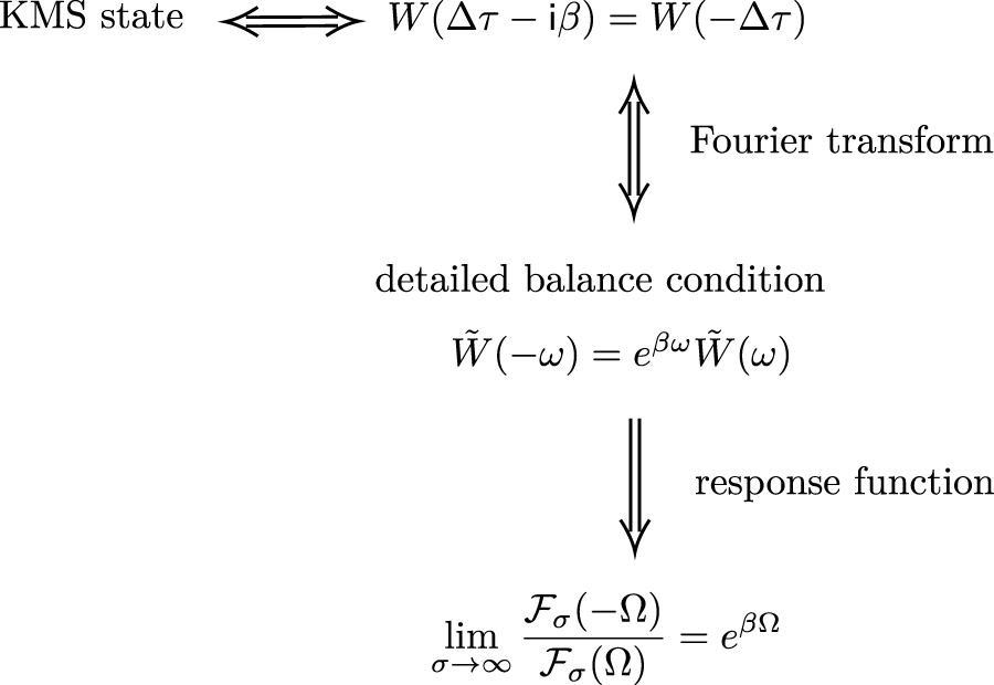
FIGURE 1. Relationship between the KMS state and the response function.

We consider a Wightman function in a field state ρ_ϕ:

$W\left(\tau ,{\tau }^{\prime }\right)={⟨\widehat{\varphi }\left(\mathsf{x}\left(\tau \right)\right)\widehat{\varphi }\left(\mathsf{x}\left({\tau }^{\prime }\right)\right)⟩}_{{\rho }_{\varphi }}.(2.14)$

It should be noted that the vacuum Wightman function $⟨0|\widehat{\varphi }(\mathsf{x}(\tau ))\widehat{\varphi }(\mathsf{x}({\tau }^{\prime }))|0⟩$ is a special case corresponding to ρ_ϕ = |0⟩⟨0|. The Wightman function satisfies the KMS condition with respect to time τ at the KMS temperature ${\beta }_{\text{KMS}}^{-1}\equiv T_{\text{KMS}}$ if

$W\left(\tau -\mathsf{i}{\beta }_{\text{KMS}},{\tau }^{\prime }\right)=W\left({\tau }^{\prime },\tau \right).(2.15)$

In addition, if the KMS condition is satisfied, then the Wightman function is stationary; i.e., it only depends on the difference in time: W(τ, τ′) = W(Δτ). We identify the KMS temperature T_KMS as the temperature of the quantum field.

The KMS condition is related to the so-called detailed balance condition. For any function f(ω), the detailed balance condition at temperature β⁻¹ is given by

$f\left(-\omega \right)=e^{\beta \omega }f\left(\omega \right).(2.16)$

It is known [31] that, assuming the Wightman function is stationary, the KMS condition with respect to τ at temperature ${\beta }_{\text{KMS}}^{-1}$ is satisfied if and only if the Fourier-transformed Wightman function,

$\tilde{W}\left(\omega \right):={\int }_{\mathbb{R}}\text{d}\mathrm{\Delta }\tau W\left(\mathrm{\Delta }\tau \right)e^{-\mathsf{i}\omega \mathrm{\Delta }\tau },(2.17)$

satisfies the detailed balance condition (Eq. 2.16).

The detailed balance condition can be implemented into the response function of a UDW detector. Suppose the Wightman function satisfies the KMS condition and the switching function χ(τ/σ) has a typical interaction duration time scale σ. The response function (Eq. 2.13) can be written as

${\mathcal{F}}_{\sigma }\left(\mathrm{\Omega }\right)={\int }_{\mathbb{R}}\frac{\text{d}\bar{\omega }}{2\pi }|\tilde{\chi }\left(\bar{\omega }\right){|}^2\tilde{W}\left(\mathrm{\Omega }+\bar{\omega }/\sigma \right),(2.18)$

where $\bar{\omega }$ is a dimensionless variable and $\tilde{\chi }(\bar{\omega })$ is the Fourier transform of the switching function χ(τ/σ). One can show that if $\tilde{\chi }(\bar{\omega })$ decays sufficiently fast as $\bar{\omega }$ increases (such as a Gaussian switching), then the response function satisfies the detailed balance condition in the long interaction limit [31, 32]:

${\displaystyle \underset{\sigma \to \infty }{\lim }}\frac{{\mathcal{F}}_{\sigma }\left(-\mathrm{\Omega }\right)}{{\mathcal{F}}_{\sigma }\left(\mathrm{\Omega }\right)}=e^{{\beta }_{\text{KMS}}\mathrm{\Omega }}.(2.19)$

Inspired by the detailed balance condition for the response function (Eq. 2.19), one may define the effective temperature T_eff:

$T_{\text{eff}}^{-1}:=\frac{1}{\mathrm{\Omega }}\ln \frac{{\mathcal{F}}_{\sigma }\left(-\mathrm{\Omega }\right)}{{\mathcal{F}}_{\sigma }\left(\mathrm{\Omega }\right)}.(2.20)$

The effective temperature is an estimator for the KMS temperature of the field. In particular, if the Wightman function obeys the KMS condition and the long interaction limit (σ → ∞) is taken, then the effective temperature becomes the KMS temperature due to Eq. 2.19.

3 Relativistic quantum Otto engine

3.1 Review: quantum Otto engine

In this section, we review the QOE following [3]. It should be noted that the whole system is composed of a qubit and thermal baths in the Gibbs state. In the following section, we take the following protocol and apply it to the system composed of a UDW detector interacting with a quantum scalar field in a quasi-free state; i.e., we omit the assumption that the baths are in a thermal state.

1. A qubit with energy gap Ω₁ is prepared in an initial state ρ₀ = p|e⟩⟨e| + (1 − p)|g⟩⟨g|, where p ∈ [0, 1], as shown in Figure 2.

2. The qubit undergoes an adiabatic expansion (zero heat exchange: ⟨Q₁⟩ = 0) to enlarge the energy gap from Ω₁ to Ω₂, where Ω₂ > Ω₁. The Hamiltonian of the qubit is given by $\widehat{H}(t)=\mathrm{\Omega }(t)|e\rangle \langle e|$, and so, the work carried out on the qubit is

$⟨W_1⟩=\int \text{d}t\mathrm{Tr}\left[{\rho }_0\frac{\text{d}\widehat{H}\left(t\right)}{\text{d}t}\right]=p\mathrm{\Delta }\mathrm{\Omega },(3.1)$

where ΔΩ ≔ Ω₂ − Ω₁. The qubit’s state remains ρ₀ due to the quantum adiabatic theorem.

3. The qubit interacts with a bath at temperature T_H. The qubit’s Hamiltonian $\widehat{H}={\mathrm{\Omega }}_2|e\rangle \langle e|$, is time independent and so, the work carried out on the qubit is zero: ⟨W₂⟩ = 0. After the interaction, the state becomes ρ₁ = (p + δp_H)|e⟩⟨e| + (1 − p − δp_H)|g⟩⟨g|. The first law of thermodynamics yields the dissipated heat:

$⟨Q_2⟩=\mathrm{Tr}[{\rho }_1\widehat{H}]-\mathrm{Tr}[{\rho }_0\widehat{H}]={\mathrm{\Omega }}_2\delta p_{\text{H}}.(3.2)$

FIGURE 2

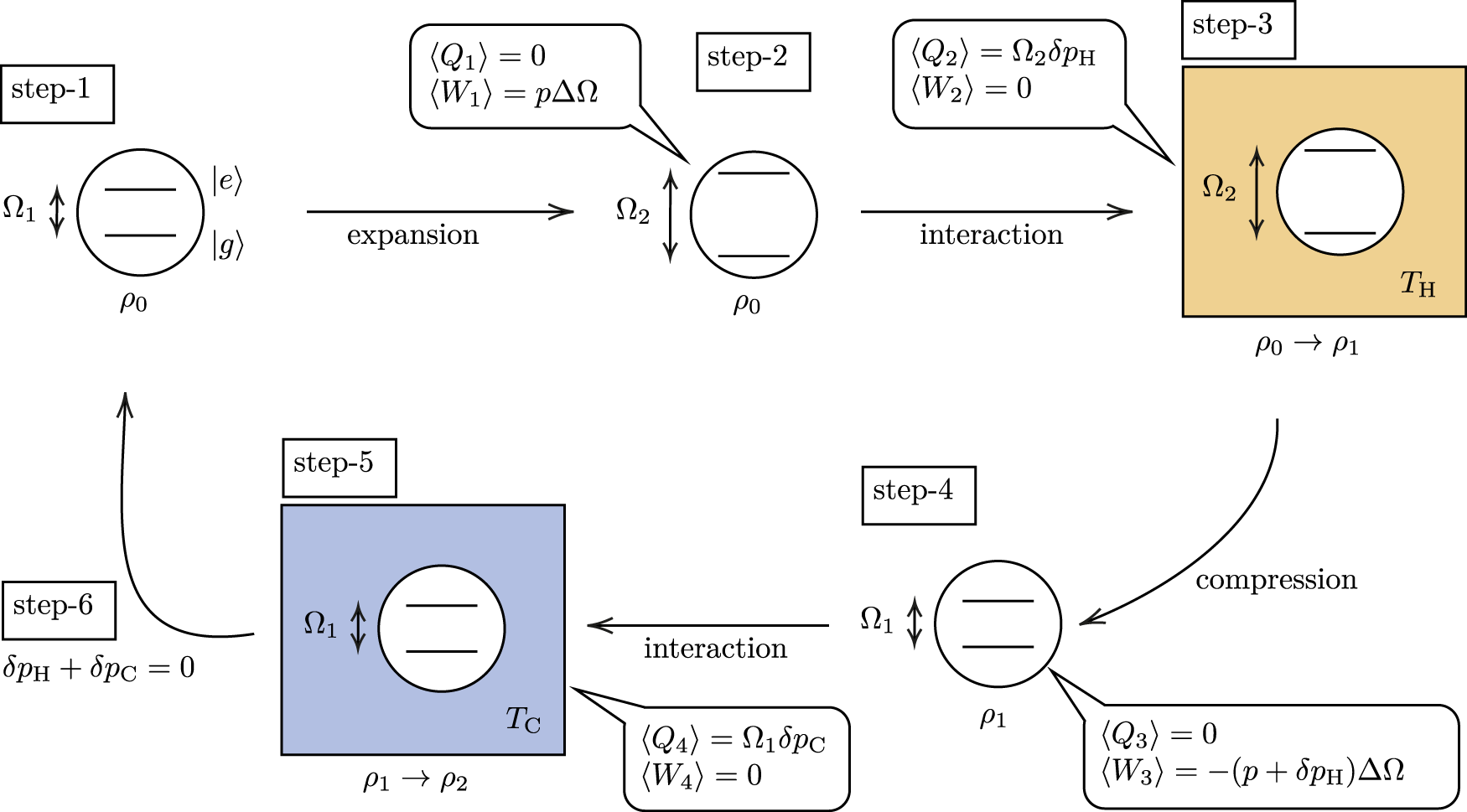
FIGURE 2. Quantum Otto cycle.

This is an isochoric thermalization process.

4. After isolating the qubit from the bath, an adiabatic contraction of the energy gap from Ω₂ to Ω₁ is performed, while the state remains ρ₁. From the same calculation as in step 2, we have

$⟨Q_3⟩=0,(3.3)$

$⟨W_3⟩=-\left(p+\delta p_{\text{H}}\right)\mathrm{\Delta }\mathrm{\Omega }.(3.4)$

The work is extracted from the qubit in this process.

5. Next, another isochoric thermalization process is carried out: the qubit interacts with a bath at a colder temperature T_C(<T_H). At the end of the process, the state becomes ρ₂ = (p + δp_H + δp_C)|e⟩⟨e| + (1 − p − δp_H − δp_C)|g⟩⟨g|, and so,

$⟨Q_4⟩={\mathrm{\Omega }}_1\delta p_{\text{C}},(3.5)$

$⟨W_4⟩=0.(3.6)$

The total extracted work and dissipated heat read

$⟨W_{\text{ext}}⟩=-{\displaystyle \sum _{j=1}^4}⟨W_j⟩=\delta p_{\text{H}}\mathrm{\Delta }\mathrm{\Omega },(3.7)$

$⟨Q⟩={\displaystyle \sum _{j=1}^4}⟨Q_j⟩={\mathrm{\Omega }}_2\delta p_{\text{H}}+{\mathrm{\Omega }}_1\delta p_{\text{C}}.(3.8)$

Assuming that Ω₂ > Ω₁, the extracted work is positive if δp_H > 0.

6. δp_H + δp_C = 0 is imposed to complete a thermodynamic cycle. From this condition, Eqs 3.7, 3.8 yield ⟨Q⟩ = ⟨W_ext⟩, which obeys the first law of thermodynamics.

It is known that the positive work condition reads [2, 3] T_C/Ω₁ < T_H/Ω₂ and the efficiency of the QOE is η_O: = ⟨W_ext⟩/Q₂ = 1 − Ω₁/Ω₂.

3.2 Work extracted by a UDW detector

Now, let us employ a UDW detector as the qubit in this process. As mentioned previously, we do not assume that the baths are thermal. Instead, we only assume that the quantum field is in a quasi-free state, i.e., the one-point correlators ${⟨\widehat{\varphi }(\mathsf{x})⟩}_{{\rho }_{\varphi }}$ vanish. Nevertheless, we continue using subscripts such as δp_H and δp_C for convenience.

In this section, we consider a general scenario in which a UDW detector following an arbitrary path in spacetime interacts with a quantum field in a quasi-free state. Working perturbatively, we derive the extracted work and the condition for it to be positive.

3.2.1 Relativistic quantum Otto engine

We first describe our QOE in the relativistic setting, as shown in Figure 3.

• Step 1: Before the interaction, the detector with the energy gap Ω₁ is prepared in ρ_D,0 in (2.9).

• Step 2: One performs a quantum adiabatic expansion Ω₁ → Ω₂ with Ω₂ > Ω₁. During this process, the detector does not interact with the field.

• Step 3: Isochoric process. The detector interacts with the field with a time dependence specified by a compactly supported switching function χ_H[(τ − τ_H)/σ_H], where τ_H is the center of interaction and σ_H(>0) is the interaction duration; its support is supp(χ_H) = [τ_H − σ_H/2, τ_H + σ_H/2]. The state changes from ρ_D,0 → ρ_D,1, where ρ_D,1 is given by Eqs 2.11–2.13, i.e.,

${\rho }_{\text{D,}1}=\left(p+\delta p_{\text{H}}\right)|e\rangle \langle e|+\left(1-p-\delta p_{\text{H}}\right)|g\rangle \langle g|+\mathcal{O}\left({\lambda }^4\right),(\mathrm{3.9a})$

$\delta p_{\text{H}}={\lambda }^2{\sigma }_{\text{H}}\left[\left(1-p\right){\mathcal{F}}_{\text{H}}\left({\mathrm{\Omega }}_2\right)-p{\mathcal{F}}_{\text{H}}\left(-{\mathrm{\Omega }}_2\right)\right],(\mathrm{3.9b})$

${\mathcal{F}}_{\text{H}}\left({\mathrm{\Omega }}_2\right)=\frac{1}{{\sigma }_{\text{H}}}{\int }_{\mathbb{R}}\text{d}\tau {\int }_{\mathbb{R}}\text{d}{\tau }^{\prime }{\chi }_{\text{H}}\left(\frac{\tau -{\tau }_{\text{H}}}{{\sigma }_{\text{H}}}\right){\chi }_{\text{H}}\left(\frac{{\tau }^{\prime }-{\tau }_{\text{H}}}{{\sigma }_{\text{H}}}\right)e^{-\mathsf{i}{\mathrm{\Omega }}_2\left(\tau -{\tau }^{\prime }\right)}W\left(\mathsf{x}\left(\tau \right),\mathsf{x}\left({\tau }^{\prime }\right)\right).(\mathrm{3.9c})$

FIGURE 3

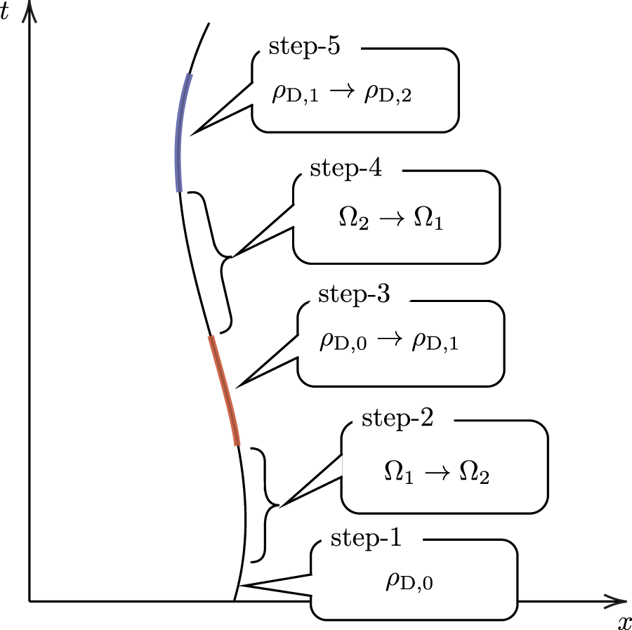
FIGURE 3. Each step in a relativistic QOE. The red and blue stripes indicate the isochoric process, i.e., the interaction between the detector and the field.

Although we identified the switching function as a compactly supported function, it is also possible to employ rapidly decreasing functions such as Gaussian or Lorentzian functions. These are not compactly supported, but the results remain unchanged when the exponentially decreasing tails of these functions are disregarded. We use these functions later in this section.

• Step 4: Adiabatic compression Ω₂ → Ω₁. Again, the detector does not interact during this process, and so, the state remains ρ_D,1.

• Step 5: Another isochoric process is implemented using χ_C[(τ − τ_C)/σ_C] for the switching function. To ensure that the interaction does not overlap with the previous isochoric process, we ensure that the supports of the two switching functions are disjoint by implementing τ_H + σ_H/2 < τ_C − σ_C/2. The state of the detector changes as ρ_D,1 → ρ_D,2, where ρ_D,2 = (p + δp_H + δp_C)|e⟩⟨e| + (1 − p − δp_H − δp_C)|g⟩⟨g|. The quantity δp_C is

$\delta p_{\text{C}}={\lambda }^2{\sigma }_{\text{C}}\left[\left(1-p-\delta p_{\text{H}}\right){\mathcal{F}}_{\text{C}}\left({\mathrm{\Omega }}_1\right)-\left(p+\delta p_{\text{H}}\right){\mathcal{F}}_{\text{C}}\left(-{\mathrm{\Omega }}_1\right)\right]+\mathcal{O}\left({\lambda }^6\right),(\mathrm{3.10a})$

${\mathcal{F}}_{\text{C}}\left({\mathrm{\Omega }}_1\right)=\frac{1}{{\sigma }_{\text{C}}}{\int }_{\mathbb{R}}\text{d}\tau {\int }_{\mathbb{R}}\text{d}{\tau }^{\prime }{\chi }_{\text{C}}\left(\frac{\tau -{\tau }_{\text{C}}}{{\sigma }_{\text{C}}}\right){\chi }_{\text{C}}\left(\frac{{\tau }^{\prime }-{\tau }_{\text{C}}}{{\sigma }_{\text{C}}}\right)e^{-\mathsf{i}{\mathrm{\Omega }}_1\left(\tau -{\tau }^{\prime }\right)}W\left(\mathsf{x}\left(\tau \right),\mathsf{x}\left({\tau }^{\prime }\right)\right).(\mathrm{3.10b})$

It should be noted that δp_C contains λ⁴ terms since δp_H is of the order λ². As in the traditional QOE, the work extracted reads ⟨W_ext⟩ = δp_HΔΩ.

• Step 6: Finally, we impose the condition δp_H + δp_C = 0 to complete a thermodynamic cycle.

Since ⟨W_ext⟩ only depends on δp_H, it may appear that the cyclicity condition does not affect this value. However there is a subtlety. If we assume that an experimenter can freely choose a value of p ∈ [0, 1] at the beginning of the cycle, this means that the experimenter has to adjust the response functions ${\mathcal{F}}_{\text{H}}(\pm {\mathrm{\Omega }}_2)$ and ${\mathcal{F}}_{\text{C}}(\pm {\mathrm{\Omega }}_1)$ in such a way that the cyclicity condition is satisfied. On the other hand, if we allow the response functions to take any value, then the population p has to be adjusted accordingly.

3.2.2 When p is free to choose

We first require the cyclicity condition, δp_H + δp_C = 0, to close the thermodynamic cycle. Since δp_C contains terms of order $\mathcal{O}({\lambda }^4)$, we omit these by imposing 1 ≫ δp_H/p for a given p( ≠ 0). This reduces to

$p\gg \frac{{\lambda }^2{\sigma }_{\text{H}}{\mathcal{F}}_{\text{H}}\left({\mathrm{\Omega }}_2\right)}{1+{\lambda }^2{\sigma }_{\text{H}}\left[{\mathcal{F}}_{\text{H}}\left({\mathrm{\Omega }}_2\right)+{\mathcal{F}}_{\text{H}}\left(-{\mathrm{\Omega }}_2\right)\right]}.(3.11)$

In particular, if the long interaction limit σ_H → ∞ is taken, we obtain

$p\gg \frac{1}{1+{\displaystyle \underset{{\sigma }_{\text{H}}\to \infty }{\lim }}{\mathcal{F}}_{\text{H}}\left(-{\mathrm{\Omega }}_2\right)/{\mathcal{F}}_{\text{H}}\left({\mathrm{\Omega }}_2\right)}=\frac{1}{1+{\displaystyle \underset{{\sigma }_{\text{H}}\to \infty }{\lim }}{e}^{{\mathrm{\Omega }}_2/T_{\text{H}}^{\text{eff}}}}.(3.12)$

Thus, for long interaction duration, $T_{\text{H}}^{\text{eff}}/{\mathrm{\Omega }}_2\ll 1$ is required. Moreover, as a special case of a detector with a rapidly decreasing switching function interacting with the quantum field in the KMS state, this reads

$p\gg \frac{1}{1+e^{{\mathrm{\Omega }}_2/T_{\text{H}}^{\text{KMS}}}}.(3.13)$

Nevertheless, if the interaction duration is finite, then λ ≪ 1 is sufficient for our perturbative analysis.²

Under this restriction, the cyclicity condition for any p ∈ (0, 1] leads to

${\sigma }_{\text{C}}{\mathcal{F}}_{\text{C}}\left({\mathrm{\Omega }}_1\right)\left(\frac{1-p}{p}-\frac{{\mathcal{F}}_{\text{C}}\left(-{\mathrm{\Omega }}_1\right)}{{\mathcal{F}}_{\text{C}}\left({\mathrm{\Omega }}_1\right)}\right)=-{\sigma }_{\text{H}}{\mathcal{F}}_{\text{H}}\left({\mathrm{\Omega }}_2\right)\left(\frac{1-p}{p}-\frac{{\mathcal{F}}_{\text{H}}\left(-{\mathrm{\Omega }}_2\right)}{{\mathcal{F}}_{\text{H}}\left({\mathrm{\Omega }}_2\right)}\right).(3.14)$

That is, one has to tune the response functions so that this equality is satisfied.

We then consider the positive work condition in the case where the value of p is chosen freely by an experimenter. The work extracted (Eq. 3.7) is

$⟨W_{\text{ext}}⟩={\lambda }^2{\sigma }_{\text{H}}\left[\left(1-p\right){\mathcal{F}}_{\text{H}}\left({\mathrm{\Omega }}_2\right)-p{\mathcal{F}}_{\text{H}}\left(-{\mathrm{\Omega }}_2\right)\right]\mathrm{\Delta }\mathrm{\Omega },(3.15)$

and the positive work condition is $(1-p){\mathcal{F}}_{\text{H}}({\mathrm{\Omega }}_2)-p{\mathcal{F}}_{\text{H}}(-{\mathrm{\Omega }}_2)>0$, i.e., $(1-p)/p>{\mathcal{F}}_{\text{H}}(-{\mathrm{\Omega }}_2)/{\mathcal{F}}_{\text{H}}({\mathrm{\Omega }}_2)$. We note that ${\mathcal{F}}_{\text{H}}(-{\mathrm{\Omega }}_2)/{\mathcal{F}}_{\text{H}}({\mathrm{\Omega }}_2)>1$ since the de-excitation probability is higher than the excitation probability, thereby implying p ∈ (0, 1/2). This is consistent with previous work [13], where the Unruh QOE with a free p can extract work only when 0 < p < 1/2. The condition can be written in terms of the effective temperature (Eq. 2.20):

${\left(\ln \frac{1-p}{p}\right)}^{-1}<\frac{T_{\text{H}}^{\text{eff}}}{{\mathrm{\Omega }}_2},\left(0<p<1/2\right).(3.16)$

It should be recalled that in the long interaction duration, $T_{\text{H}}^{\text{eff}}/{\mathrm{\Omega }}_2\ll 1$ is required, which means that Eq. 3.16 tells us that p ≪ 1 needs to be chosen if we wish to extract positive work in the long interaction limit within the perturbation theory.

It should be noted that if the positive work is extracted while the cyclicity condition is satisfied, then ${\mathcal{F}}_{\text{C}}(\pm {\mathrm{\Omega }}_1)$ has to obey $(1-p)/p<{\mathcal{F}}_{\text{C}}(-{\mathrm{\Omega }}_1)/{\mathcal{F}}_{\text{C}}({\mathrm{\Omega }}_1)$ since the response functions are non-negative and the positive work condition requires $(1-p)/p>{\mathcal{F}}_{\text{H}}(-{\mathrm{\Omega }}_2)/{\mathcal{F}}_{\text{H}}({\mathrm{\Omega }}_2)$. Therefore, within the perturbation theory,

$⟨W_{\text{ext}}⟩>0\text{from\hspace{0.17em}QOE}\Rightarrow \frac{T_{\text{C}}^{\text{eff}}}{{\mathrm{\Omega }}_1}<{\left(\ln \frac{1-p}{p}\right)}^{-1}<\frac{T_{\text{H}}^{\text{eff}}}{{\mathrm{\Omega }}_2}.(3.17)$

The opposite is not always true since the inequality does not necessarily imply the cyclicity condition (3.14). In addition, the statement (3.17) does not hold without the cyclicity condition. Nevertheless, by contraposition, if $T_{\text{H}}^{\text{eff}}/{\mathrm{\Omega }}_2>T_{\text{C}}^{\text{eff}}/{\mathrm{\Omega }}_1$ is violated, then positive work cannot be extracted or the cycle is not closed.

The inequality $T_{\text{H}}^{\text{eff}}/{\mathrm{\Omega }}_2>T_{\text{C}}^{\text{eff}}/{\mathrm{\Omega }}_1$ generalizes the positive work condition found in [2, 3], by replacing bath temperatures with effective temperatures. Specifically, effective temperatures reduce to the KMS temperatures when the pullback of the Wightman function along a trajectory satisfies the KMS condition and when the detector, with a rapidly decreasing switching function, interacts with the field for a long time. In this particular scenario, the work extracted becomes

$⟨W_{\text{ext}}⟩\approx {\lambda }^2{\sigma }_{\text{H}}{\mathcal{F}}_{\text{H}}\left({\mathrm{\Omega }}_2\right)\left[1-p\left(1+e^{{\mathrm{\Omega }}_2/T_{\text{H}}^{\text{KMS}}}\right)\right]\mathrm{\Delta }\mathrm{\Omega }.(3.18)$

3.2.3 When p is adjusted

Let us focus on the case where p is initially adjusted and derive the work extracted. We again assume that p ≠ 0 and p ≫ δp_H so that the terms higher than λ⁴ can be omitted in δp_C. From the cyclicity condition, we can solve for p, which reads

$p=\frac{{\sigma }_{\text{H}}{\mathcal{F}}_{\text{H}}\left({\mathrm{\Omega }}_2\right)+{\sigma }_{\text{C}}{\mathcal{F}}_{\text{C}}\left({\mathrm{\Omega }}_1\right)}{{\sigma }_{\text{H}}\left[{\mathcal{F}}_{\text{H}}\left({\mathrm{\Omega }}_2\right)+{\mathcal{F}}_{\text{H}}\left(-{\mathrm{\Omega }}_2\right)\right]+{\sigma }_{\text{C}}\left[{\mathcal{F}}_{\text{C}}\left({\mathrm{\Omega }}_1\right)+{\mathcal{F}}_{\text{C}}\left(-{\mathrm{\Omega }}_1\right)\right]}.(3.19)$

By inserting p into Eq. 3.7, we obtain

$⟨W_{\text{ext}}⟩={\lambda }^2{\sigma }_{\text{H}}{\sigma }_{\text{C}}\frac{{\mathcal{F}}_{\text{H}}\left({\mathrm{\Omega }}_2\right){\mathcal{F}}_{\text{C}}\left(-{\mathrm{\Omega }}_1\right)-{\mathcal{F}}_{\text{H}}\left(-{\mathrm{\Omega }}_2\right){\mathcal{F}}_{\text{C}}\left({\mathrm{\Omega }}_1\right)}{{\sigma }_{\text{H}}\left[{\mathcal{F}}_{\text{H}}\left({\mathrm{\Omega }}_2\right)+{\mathcal{F}}_{\text{H}}\left(-{\mathrm{\Omega }}_2\right)\right]+{\sigma }_{\text{C}}\left[{\mathcal{F}}_{\text{C}}\left({\mathrm{\Omega }}_1\right)+{\mathcal{F}}_{\text{C}}\left(-{\mathrm{\Omega }}_1\right)\right]}\mathrm{\Delta }\mathrm{\Omega }.(3.20)$

The extracted work is positive if and only if

${\mathcal{F}}_{\text{H}}\left({\mathrm{\Omega }}_2\right){\mathcal{F}}_{\text{C}}\left(-{\mathrm{\Omega }}_1\right)>{\mathcal{F}}_{\text{H}}\left(-{\mathrm{\Omega }}_2\right){\mathcal{F}}_{\text{C}}\left({\mathrm{\Omega }}_1\right).(3.21)$

We find that the positive work condition (Eq. 3.21) can be written in terms of the effective temperature defined by Eq. 2.20 as

$\frac{T_{\text{C}}^{\text{eff}}}{{\mathrm{\Omega }}_1}<\frac{T_{\text{H}}^{\text{eff}}}{{\mathrm{\Omega }}_2}.(3.22)$

Again, we are not necessarily assuming that the field is in the KMS state, and so, the effective temperature is not necessarily the KMS temperature. If the field is in the KMS state and the detector with a rapidly decreasing switching function interacts with the field for a long time (σ_H, σ_C → ∞), the effective temperature becomes the KMS temperature, leading to

$\frac{T_{\text{C}}^{\text{KMS}}}{{\mathrm{\Omega }}_1}<\frac{T_{\text{H}}^{\text{KMS}}}{{\mathrm{\Omega }}_2},(3.23)$

which is the condition found in [2, 3]. The extracted work in this case is

$⟨W_{\text{ext}}⟩={\lambda }^2{\sigma }_{\text{H}}{\sigma }_{\text{C}}\frac{\left(e^{{\mathrm{\Omega }}_1/T_{\text{C}}}-e^{{\mathrm{\Omega }}_2/T_{\text{H}}}\right){\mathcal{F}}_{\text{H}}\left({\mathrm{\Omega }}_2\right){\mathcal{F}}_{\text{C}}\left({\mathrm{\Omega }}_1\right)}{{\sigma }_{\text{H}}\left(1+e^{{\mathrm{\Omega }}_2/T_{\text{H}}}\right){\mathcal{F}}_{\text{H}}\left({\mathrm{\Omega }}_2\right)+{\sigma }_{\text{C}}\left(1+e^{{\mathrm{\Omega }}_1/T_{\text{C}}}\right){\mathcal{F}}_{\text{C}}\left({\mathrm{\Omega }}_1\right)}\mathrm{\Delta }\mathrm{\Omega }.(3.24)$

Therefore, Eq. 3.23 is a special case of Eq. 3.21 [and equivalently (Eq. 3.22)] when the response function obeys the detailed balance condition (Eq. 2.19). In other words, the condition (Eq. 3.21) [or alternatively (Eq. 3.22)] is applicable to any scenario, even when the detector is not thermalized.

In summary, we showed that within the perturbation theory, the positive work condition is associated with $T_{\text{C}}^{\text{eff}}/{\mathrm{\Omega }}_1<T_{\text{H}}^{\text{eff}}/{\mathrm{\Omega }}_2$. If p is not fixed and the cycle is closed by adjusting the response functions, $T_{\text{C}}^{\text{eff}}/{\mathrm{\Omega }}_1<T_{\text{H}}^{\text{eff}}/{\mathrm{\Omega }}_2$ is a necessary condition to extract positive work. On the other hand, if we instead adjust p to close the cycle while the response functions are not fixed, then this condition is necessary and sufficient. This recovers the traditional QOE positive work condition [2, 3] as a special case. It should be noted that our results hold not only for a quantum field in the KMS state but also for any quasi-free state in curved spacetime. The use of the effective temperature is similar to that in other papers such as [33].

4 Examples

We now demonstrate our results in (3 + 1)-dimensional Minkowski spacetime. Throughout this section, we use a Gaussian switching function

$\chi \left[\left.\left(\tau -{\tau }_j\right)/\sigma \right)\right]=e^{-{\left(\tau -{\tau }_j\right)}^2/2{\sigma }^2},j\in \left\{\text{H},\text{C}\right\},(4.1)$

where τ_j is the center of the Gaussian and σ > 0 is the characteristic Gaussian width, which has the units of time.

4.1 Inertial detector in the thermal quantum field

Consider (3 + 1)-dimensional Minkowski spacetime. We aim to examine the extracted work (Eq. 3.20) by coupling an inertial UDW detector to a KMS state of the field to explore the basic properties of the work extraction.

The Wightman function in a thermal state of a massless field can be written as [34]

$W_{\beta }\left(\mathsf{x},{\mathsf{x}}^{\prime }\right)=W_{\text{M}}\left(\mathsf{x},{\mathsf{x}}^{\prime }\right)+W_{\text{th}}\left(\mathsf{x},{\mathsf{x}}^{\prime }\right),(4.2)$

where W_M is the Wightman function in the Minkowski vacuum and W_th is the contribution from the thermal state:

$W_{\text{M}}\left(\mathsf{x},{\mathsf{x}}^{\prime }\right)=-\frac{1}{4{\pi }^2}\frac{1}{{\left(t-t^{\prime }-\mathsf{i}ϵ\right)}^2-|\mathit{x}-{\mathit{x}}^{\prime }{|}^2},(\mathrm{4.3a})$

$W_{\text{th}}\left(\mathsf{x},{\mathsf{x}}^{\prime }\right)={\int }_{{\mathbb{R}}^3}\frac{{\text{d}}^{3}k}{{\left(2\pi \right)}^{3}2|\mathit{k}|}\frac{e^{\mathsf{i}|\mathit{k}|\left(t-t^{\prime }\right)-\mathsf{i}\mathit{k}\cdot \left(\mathit{x}-{\mathit{x}}^{\prime }\right)}+\text{c.c.}}{e^{\beta |\mathit{k}|}-1}.(\mathrm{4.3b})$

Here, ϵ is the UV cutoff and β = T⁻¹ is the inverse KMS temperature of the field.

Assuming the Gaussian switching (Eq. 4.1), the response function ${\mathcal{F}}_{\beta }(\mathrm{\Omega })$ of an inertial detector in the thermal bath reads [34]

${\mathcal{F}}_{\beta }\left(\mathrm{\Omega }\right)={\mathcal{F}}_{\text{M}}\left(\mathrm{\Omega }\right)+{\mathcal{F}}_{\text{th}}\left(\mathrm{\Omega }\right),(4.4)$

where

${\mathcal{F}}_{\text{M}}\left(\mathrm{\Omega }\right)=\frac{1}{4\pi \sigma }\left[e^{-{\mathrm{\Omega }}^2{\sigma }^2}-\sqrt{\pi }\mathrm{\Omega }\sigma \text{erfc}\left(\mathrm{\Omega }\sigma \right)\right],(\mathrm{4.5a})$

${\mathcal{F}}_{\text{th}}\left(\mathrm{\Omega }\right)=\frac{e^{-{\mathrm{\Omega }}^2{\sigma }^2}\sigma }{\pi }{\int }_0^{\infty }\text{d}k\frac{k{e}^{-k^2{\sigma }^2}\cosh \left(2\mathrm{\Omega }{\sigma }^{2}k\right)}{e^{\beta k}-1}(\mathrm{4.5b})$

are the response functions for an inertial detector in the Minkowski vacuum and the thermal contribution, respectively. It should be noted that it does not depend on the center of the Gaussian switching since the Wightman function is time-translation invariant. We assume that the interaction durations are the same: σ_H = σ_C ≡ σ.

4.1.1 Case: free choice of p

We first consider the case where p is freely chosen, as discussed in Section 3.2.2. We plot ⟨W_ext⟩/λ²σ defined in Eq. 3.15 as a function of interaction duration σ when T_H = 2, Ω₂ = 3, p = 0.315 and Ω₁ = 1 in Figure 4Ai. The dashed line represents the asymptotic value, lim_σ→∞⟨W_ext⟩/λ²σ, given by Eq. 3.18. We observe that the work can be extracted when the interaction duration is short, but as σ increases, extraction becomes exponentially difficult. This behavior can be explained by examining the positive work condition (Eq. 3.16) in Figure 4Aii. The figure shows that the positive work condition is satisfied when σ is small enough. When σ → ∞ is taken, the effective temperature becomes the KMS temperature: $T_{\text{H}}^{\text{eff}}/{\mathrm{\Omega }}_2\to T_{\text{H}}/{\mathrm{\Omega }}_2=2/3$ in Figure 4Aii. Moreover, based on the discussion in Section 3.2.2, the perturbative analysis is valid in this limit when T_H/Ω₂ ≪ 1, which is not the case in our scenario. Nevertheless, the perturbative analysis is valid in the figure as long as λ ≪ 1.

FIGURE 4

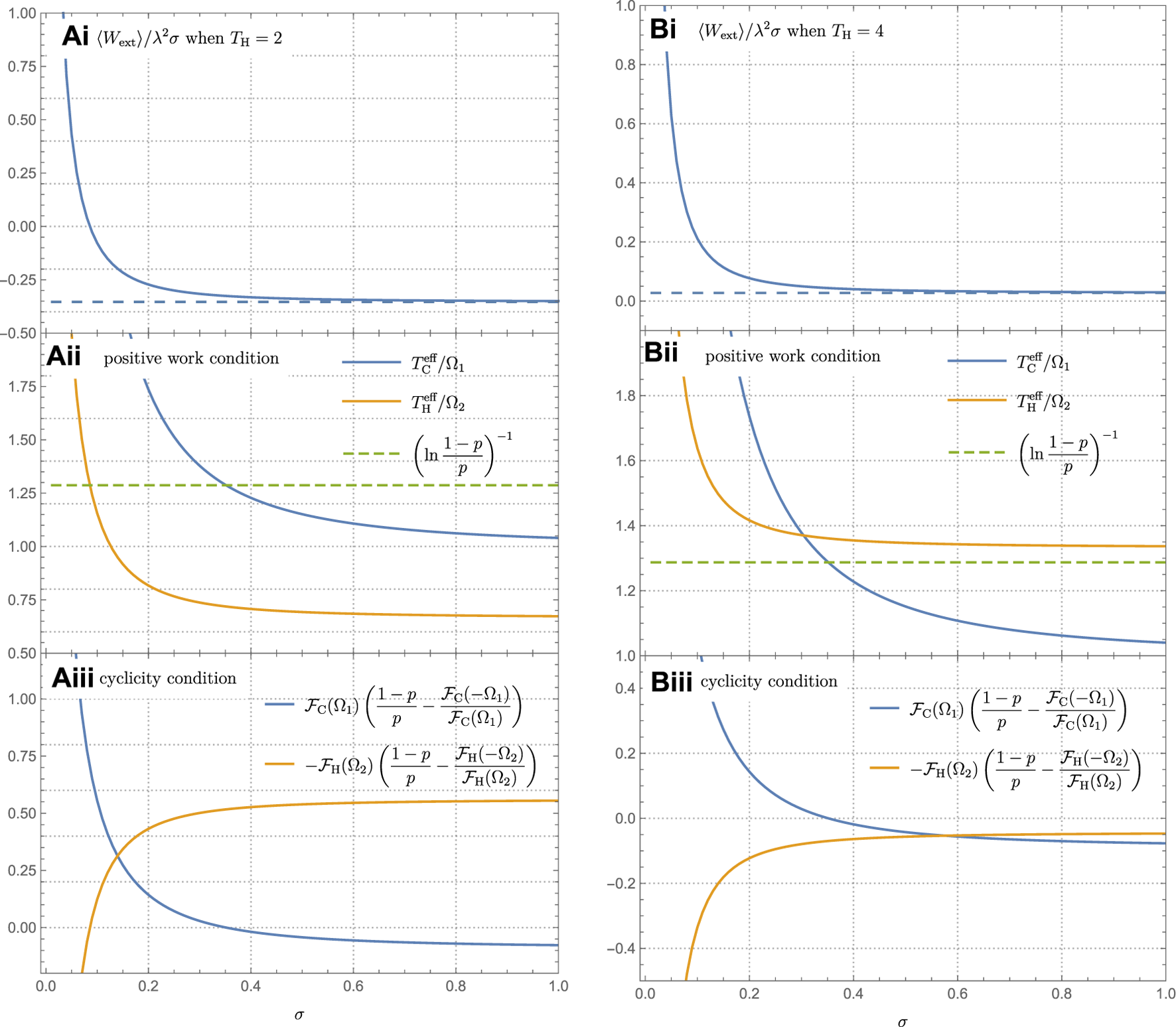
FIGURE 4. Extracted work and conditions for a UDW detector in a KMS state of a thermal quantum field for (A) T_H = 2 and (B) T_H = 4. Here, Ω₂ = 3, T_C = 1, and p = 0.315 in units of Ω₁. (Ai) and (Bi) depict ⟨W_ext⟩/λ²σ as a function of the interaction duration σ in units of Ω₁. The dashed line indicates the asymptotic value. The positive work condition is examined in (Aii) and (Bii), and the cyclicity condition is investigated in (Aiii) and (Biii). Negative values mean that work is carried out on the system (i.e., the UDW detector).

Although ⟨W_ext⟩/λ²σ > 0 for some σ, the thermodynamic cycle is not closed. The cyclicity condition (Eq. 3.14) when σ_H = σ_C reads

${\mathcal{F}}_{\text{C}}\left({\mathrm{\Omega }}_1\right)\left(\frac{1-p}{p}-\frac{{\mathcal{F}}_{\text{C}}\left(-{\mathrm{\Omega }}_1\right)}{{\mathcal{F}}_{\text{C}}\left({\mathrm{\Omega }}_1\right)}\right)=-{\mathcal{F}}_{\text{H}}\left({\mathrm{\Omega }}_2\right)\left(\frac{1-p}{p}-\frac{{\mathcal{F}}_{\text{H}}\left(-{\mathrm{\Omega }}_2\right)}{{\mathcal{F}}_{\text{H}}\left({\mathrm{\Omega }}_2\right)}\right).(4.6)$

We plot each side of this equation in Figure 4Aiii, fixing T_C = 1 and other parameters (except σ) so as to find an optimal interaction duration σ such that the two curves cross. This point in the figure represents the scenario when the cyclicity condition is satisfied. As one can see, the positive work condition in Figure 4Aii and the cyclicity condition in 4Aiii are not satisfied at the same time; hence, the work extracted does not come from a genuine QOE. In fact, Figure 4Aii shows us that $T_{\text{C}}^{\text{eff}}/{\mathrm{\Omega }}_1>T_{\text{H}}^{\text{eff}}/{\mathrm{\Omega }}_2$, and the statement (Eq. 3.17) implies that either work cannot be extracted or that the thermodynamic cycle is not closed.

Meanwhile, we can find a set of parameters that enables us to extract positive work from a closed QOE. This scenario is shown in Figure 4B, where T_H = 4 is chosen. Figure 4Bi shows that the extracted work is positive for all σ, which is consistent with the positive work condition examined in Figure 4Bii. This time, from Figure 4Biii, there exists a value of σ that satisfies the cyclicity condition while ⟨W_ext⟩/λ²σ > 0. Moreover, Figures 4Bii, iii exemplify the statement (Eq. 3.17): if positive work is extracted from a genuine QOE, then the effective temperatures satisfy $T_{\text{C}}^{\text{eff}}/{\mathrm{\Omega }}_1<1/\ln [(1-p)/p]<T_{\text{H}}^{\text{eff}}/{\mathrm{\Omega }}_2$, but the opposite is not always true.

4.1.2 Case: adjusted p

We now consider the QOE described in Section 3.2.3. We first note that an inertial detector in the Minkowski vacuum (i.e., zero temperature: T_H = T_C = 0) cannot extract work from vacuum fluctuations since the condition (3.21) cannot be satisfied no matter what Ω and σ are. We then consider the KMS temperatures T_H, T_C ≠ 0 and compute the extracted work ⟨W_ext⟩/λ²σ. The interaction duration σ is divided so that the perturbative analysis is valid—otherwise, the extracted work ⟨W_ext⟩/λ² monotonically increases with σ without an upper bound. In Figure 5A, we plot the extracted work ⟨W_ext⟩/λ²σ as a function of σ with various T_H. Here, quantities are in units of the energy gap Ω₁ at the beginning of the cycle, and we fix Ω₂/Ω₁ = 3 and T_C/Ω₁ = 1. We observe that the detector cannot extract positive work when the interaction duration is too short (i.e., σΩ₁ ≪ 1), while ⟨W_ext⟩/λ²σ asymptotes to a number at σΩ₁ ≫ 1. This is the opposite behavior of the result shown in Figure 4, and it can be attributed to the difference between the positive work conditions given by Eqs 3.16, 3.22. In the case of free p, as shown in Figure 4B, $T_{\text{H}}^{\text{eff}}/{\mathrm{\Omega }}_2$ is compared to a constant value. In contrast, for Figure 5, $T_{\text{H}}^{\text{eff}}/{\mathrm{\Omega }}_2$ is compared to another effective temperature $T_{\text{C}}^{\text{eff}}/{\mathrm{\Omega }}_1$ as depicted in Figure 5B.

FIGURE 5

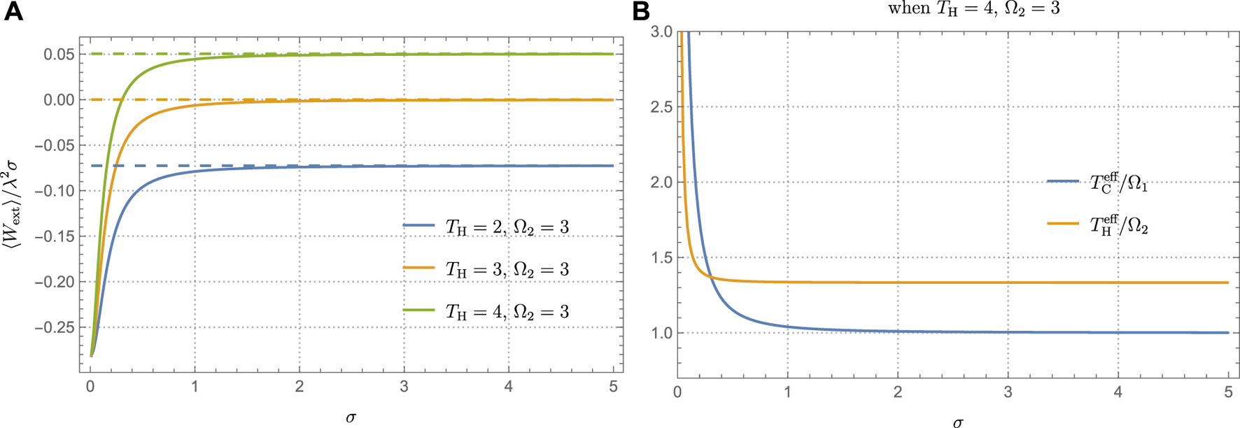
FIGURE 5. (A) Extracted work ⟨W_ext⟩/λ²σ as a function of the interaction duration σ in units of Ω₁. Here, T_C =1. The dashed lines are the work extracted (3.24) after the detailed balance condition is satisfied. (B) Effective temperature divided by the energy gap in the case of T_H = 4 and Ω₂ = 3 in (A). The positive work condition is satisfied when $T_{\text{C}}^{\text{eff}}/{\mathrm{\Omega }}_1<T_{\text{H}}^{\text{eff}}/{\mathrm{\Omega }}_2$. Negative values mean that work is carried out on the system (i.e., the UDW detector).

The asymptotic value for each curve is depicted by the dashed line in Figure 5A, which is evaluated from (3.24). This confirms that, at the long interaction duration, the detailed balance condition for the response function (2.19) is satisfied. In addition, we observe that the work extracted when (T_H/Ω₁, Ω₂/Ω₁) = (2, 3) and (3,3) is always negative, whereas it is possible to extract positive work from the system with (T_H/Ω₁, Ω₂/Ω₁) = (4, 3). This can be understood from the condition (3.23); when the detailed balance condition (2.19) is satisfied (σΩ₁ ≫ 1 in this case), the detector can extract positive work when the temperature of the baths and the energy gap obey (3.23).

4.2 UDW detector in circular motion

The Unruh QOE utilizes the thermality caused by the Unruh effect at the temperatures T_H = a_H/2π and T_C = a_C/2π with a_H > a_C in the protocol described in Section 3 [13]. However, as mentioned previously, a linearly accelerating UDW detector is not ideal for extracting thermodynamic work since it requires a tremendous amount of acceleration a as well as a huge space to let the detector travel long distances. Instead, we aim to employ a UDW detector in circular motion, which not only allows us to confine the detector in a compact space but also requires less space to acquire some temperatures compared to the linear acceleration case. Moreover, the Wightman function along a circulating detector’s trajectory does not satisfy the KMS condition. Our general expression for the extracted work (3.15) and (3.20) as well as the positive work condition (3.16) and (3.22) can still be applied to such a scenario.

We consider the circular trajectory of the UDW detector, which is given by

$\mathsf{x}\left(\tau \right)=\left\{t=\gamma \tau ,x=R\cos \left(\omega \gamma \tau \right),y=R\sin \left(\omega \gamma \tau \right),z=0\right\}.(4.7)$

Here, R( > 0) is the radius of the circle, ω is the angular velocity of the detector, and $\gamma =1/\sqrt{1-R^2{\omega }^2}$. One can introduce the proper acceleration of the detector, whose magnitude a is given by a = Rω²γ², as well as the speed of the detector v = Rω(≤1). Using these relations, one can write γ, ω, v in terms of a and R as follows:

$\omega =\sqrt{\frac{a}{\left(1+aR\right)R}},(\mathrm{4.8a})$

$\gamma =\sqrt{1+aR},(\mathrm{4.8b})$

$v=\sqrt{\frac{aR}{1+aR}}.(\mathrm{4.8c})$

In order to calculate the response function (2.13), one needs to have an expression of the pullback of the Wightman function along the trajectory (4.7). We consider a minimally coupled, massless quantum scalar field in (3 + 1)-dimensional Minkowski spacetime. The Wightman function in the Minkowski vacuum is given by Eq. 4.3a. Inserting (4.7), we obtain the pullback of the Wightman function:

$W\left(\mathsf{x}\left(\tau \right),{\mathsf{x}}^{\prime }\left({\tau }^{\prime }\right)\right)=-\frac{1}{4{\pi }^2}\frac{1}{{\gamma }^2{\left(\mathrm{\Delta }\tau -\mathsf{i}ϵ\right)}^2-4R^2{\sin }^2\left(\omega \gamma \mathrm{\Delta }\tau /2\right)},(4.9)$

where Δτ ≔ τ − τ′. Since the Wightman function is a time-translation invariant, the response functions do not depend on the switching time.

4.2.1 Extracted work

From the aforementioned Wightman function, we can numerically calculate the response functions and the work extracted for the detector in circular motion. In Figure 6, we plot ⟨W_ext⟩/λ²σ as a function of σ in units of the energy gap Ω₁ in step 1. Figures 6A, B show the cases where p is freely chosen and tuned, respectively. In both figures, we set Ω₂/Ω₁ = 1.01, RΩ₁ = 1, and a_C/Ω₁ = 1, and each figure includes the curves for a_H/Ω₁ = 2 and 3.

FIGURE 6

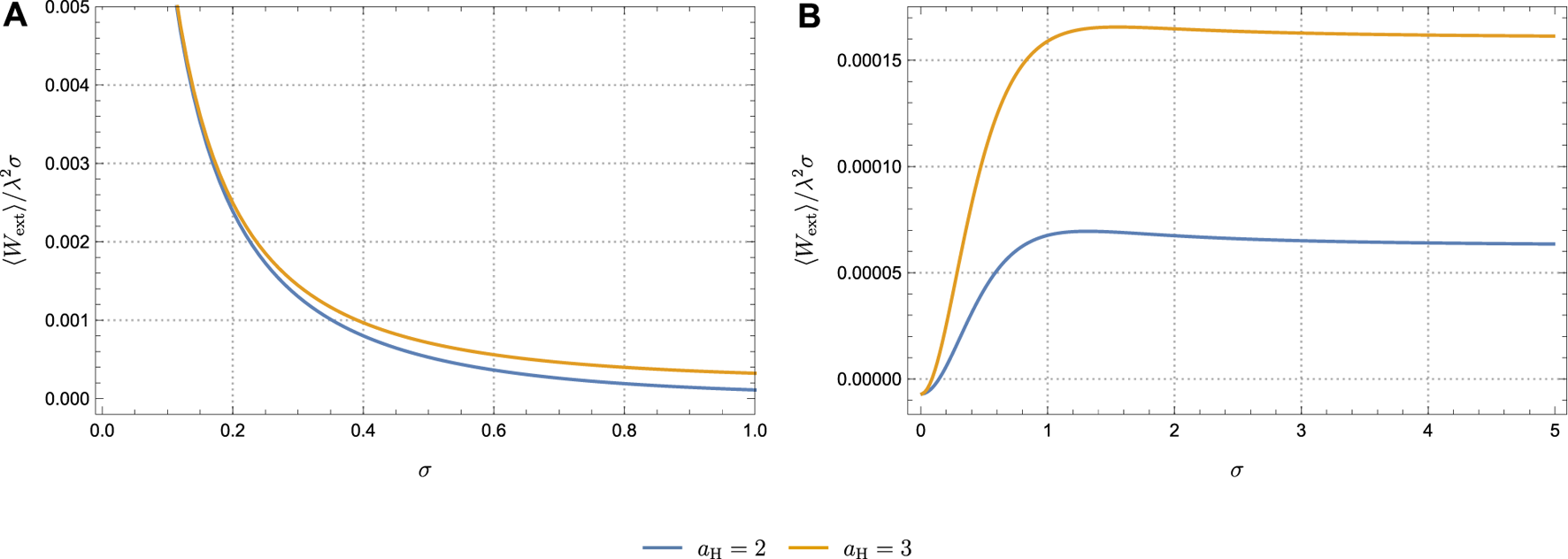
FIGURE 6. Extracted work ⟨W_ext⟩/λ²σ by a detector in circular motion as a function of the interaction duration σ in units of Ω₁. Here, Ω₂ = 1.01 and a_C = 1. (A) Case where p is adjustable and p = 1/20; (B) case where p is tuned to complete the cycle. Each figure contains a_H = 2 and a_H = 3.

As in the case of the inertial detector in a thermal bath, the QOE with a free p (here p = 1/20) extracts more work when the interaction duration is short [Figure 6A], whereas if p is tuned to close the cycle, the opposite behavior holds [Figure 6B]. However, we find that in the latter case, unlike in Section 2.2, the extracted work does not reach a maximum at large σ. Instead, there exists a maximum at σΩ₁ ≈ 1. Nevertheless, we confirm that this behavior is contingent on the choice of parameters.

We then plot ⟨W_ext⟩/λ²σ as a function of the radius of the circle, log₁₀R, in units of Ω₁ in Figure 7. Here, we set Ω₂ = 2, σ = 1, a_C = 1, and each figure includes curves for a_H = 3, 4, and 5. As mentioned before, Figure 7A corresponds to the QOE with p = 1/20, while Figure 7B depicts the result with a tuned p. Both figures exhibit a similar pattern; a detector orbiting with a small radius R has difficulty extracting work, and ⟨W_ext⟩/λ²σ is maximized as R increases, eventually asymptoting to some value at R → ∞. Thus, the radius R of the orbit must be optimized to extract the maximum amount of work.

FIGURE 7

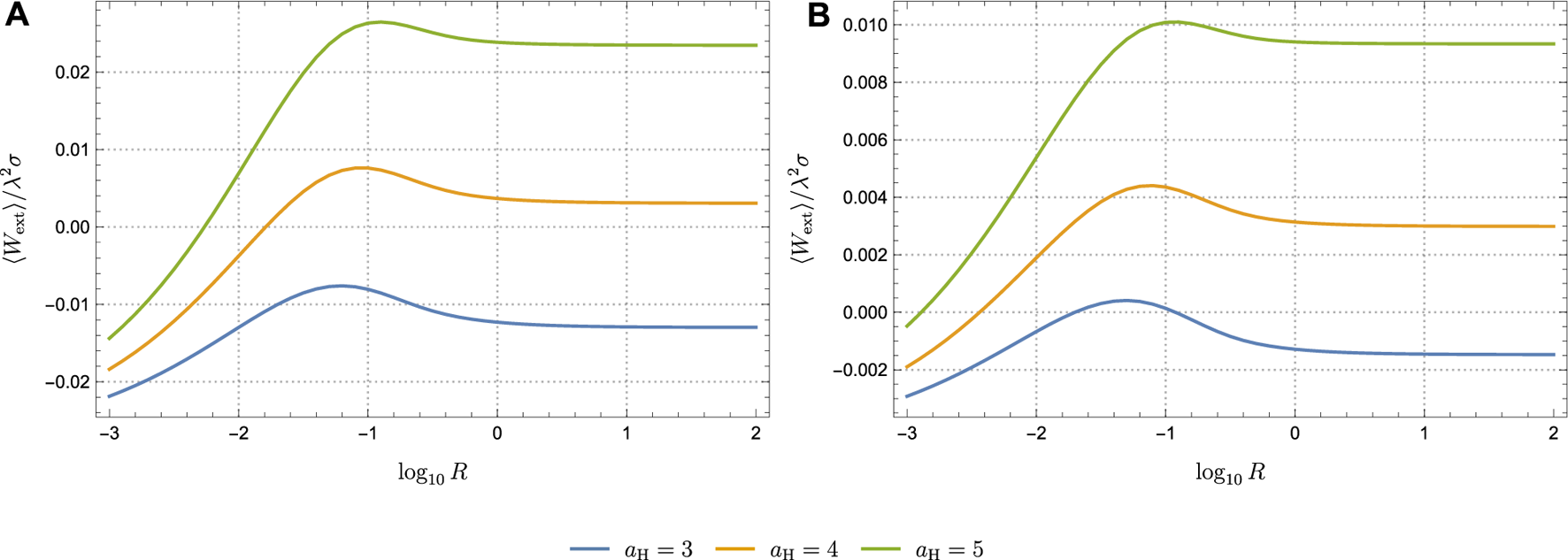
FIGURE 7. Work extracted by a circulating UDW detector as a function of the radius log₁₀R when (A) p is adjustable (chosen to be p = 1/20) and (B) p is tuned to complete the cycle. Here, Ω₂ = 2, σ = 1, and a_C = 1 in units of Ω₁. Each figure contains three cases of a_H: a_H = 3, 4, and 5. It should be noted that negative values correspond to work carried out on the system (i.e., the UDW detector).

4.2.2 Fixed acceleration

Although the analytic expression for the effective temperature for a circulating detector, T_circ, cannot be obtained in general, one can impose an additional assumption to obtain the exact form of T_circ. Suppose that the detector is circulating at high speed v ≈ 1 (i.e., ultrarelativistic regime), which can be realized by taking a large radius R. The effective temperature in this case is known to be [24, 27]

$T_{\text{circ}}=\frac{|\mathrm{\Omega }|}{\ln \left[1+\frac{4\sqrt{3}|\mathrm{\Omega }|}{a}\exp \left(\frac{2\sqrt{3}|\mathrm{\Omega }|}{a}\right)\right]}\in \left(a/4\sqrt{3},a/2\sqrt{3}\right).(4.10)$

While the effective temperature T_circ increases with a, it is also possible to enhance the temperature by enlarging the energy gap Ω with fixed acceleration. That is, for a given a, T_circ(Ω₂) > T_circ(Ω₁) if Ω₂ > Ω₁. We then ask if the detector circulating at high speed with a fixed acceleration a can extract positive work by manipulating the effective temperature by adjusting the energy gap.

The answer to this inquiry is negative. To see this, it is easy to check that, for a given a > 0, Ω₂ > Ω₁ ⇒ T_circ(Ω₂)/Ω₂ < T_circ(Ω₁)/Ω₁, which violates the necessary condition for positive work, (3.16) and (3.22). Thus, we find that, for any p ∈ (0, 1), it is impossible to extract positive work from a UDW detector in circular motion at v ≈ 1 by fixing a. This is one example of the feature of quantum heat engines: T_C < T_H does not necessarily guarantee the extraction of positive work in quantum heat engines, but rather, one should consider T_C/Ω₁ < T_H/Ω₂, where Ω₁ < Ω₂.

5 Conclusion

Inspired by the Unruh quantum Otto engines, we considered the QOE in a general setting utilizing a UDW detector interacting with a quantum scalar field. While the original QOE considered a qubit thermalized in thermal baths, we assumed that 1) the field is in a quasi-free state, not necessarily in a KMS thermal state and 2) the detector follows an arbitrary trajectory in curved spacetime. Using a perturbative method, we derived the extracted work (3.15 and 3.20) in terms of the response function of the UDW detector. In addition, we found that the condition for extracting positive work can be expressed in terms of the effective temperature perceived by the detector (3.16 and 3.22). These formulas are applicable to various scenarios outside (thermal) equilibrium. As a particular case, if the field is in the KMS state and the detector with a rapidly decreasing switching function interacts with it for a long time, the response function obeys the detailed balance condition, which makes the effective temperature identical to the KMS temperature. The condition (3.22) then becomes the positive work condition (3.23) originally found by [2, 3].

Using the formula for the extracted work, we explored two concrete examples: an inertial detector in the KMS state and a circulating detector in the Minkowski vacuum.

In the scenario of an inertial detector in thermal baths, we numerically examined the effect of the interaction duration. The relationship between the extracted work and the interaction duration is drastically changed by the choice of the detector’s initial state. Nevertheless, the extracted work asymptotes to the value that corresponds to thermal equilibrium as the interaction duration increases.

Another example involves a circulating detector in the Minkowski vacuum. The motivation for this scenario comes from the previously proposed Unruh QOE [13], in which the thermal baths are generated by the Unruh effect. However, utilizing a linearly accelerating UDW detector in the Unruh QOE is not practical for several reasons, such as the work necessary for acceleration and the requirement for a large space. The circulating detector, on the other hand, circumvents these issues. Moreover, the QOE with a circulating detector can be adequately examined only when our general framework is employed. The Wightman function pulled back along the circular trajectory does not satisfy the KMS condition, which suggests that the use of the effective temperature is necessary.

The work extracted by the circulating detector showed behavior similar to that of the inertial detector in a thermal bath. However, we found that there exist optimal values for the interaction duration and radius of the orbit to extract maximum work. Furthermore, we showed that the detector cannot extract work with a fixed acceleration due to the violation of the positive work condition.

An interesting extension to our work would involve exploring quantum heat engines using non-quasi-free states. In particular, coherent and squeezed states—which are not quasi-free—are of particular interest in a variety of settings. It would be interesting to see how a non-vanishing one-point correlator contributes to the cycle.

Data availability statement

The raw data supporting the conclusion of this article will be made available by the authors, without undue reservation.

Author contributions

KG-Y: conceptualization, formal Analysis, investigation, methodology, software, supervision, and writing–original draft and review and editing. VT: formal analysis, investigation, and writing–review and editing. RM: conceptualization, funding acquisition, investigation, methodology, supervision, and writing–review and editing.

Funding

The authors declare financial support was received for the research, authorship, and/or publication of this article. This work was supported in part by the Natural Sciences and Engineering Research Council of Canada.

Acknowledgments

KG-Y thanks Dr. Jorma Louko for the insightful discussion.

Conflict of interest

The authors declare that the research was conducted in the absence of any commercial or financial relationships that could be construed as a potential conflict of interest.

Publisher’s note

All claims expressed in this article are solely those of the authors and do not necessarily represent those of their affiliated organizations, or those of the publisher, the editors, and the reviewers. Any product that may be evaluated in this article, or claim that may be made by its manufacturer, is not guaranteed or endorsed by the publisher.

Footnotes

¹Sometimes, quasi-free states are called Gaussian states in the literature.

²To be precise, one has to make λ a dimensionless quantity since it has units of [Length]^(n−3)/2 in (n + 1) dimensions.

References

1. Scovil HED, Schulz-DuBois EO. Three-level masers as heat engines. Phys Rev Lett (1959) 2:262–3. doi:10.1103/physrevlett.2.262

CrossRef Full Text | Google Scholar

2. Feldmann T, Kosloff R. Performance of discrete heat engines and heat pumps in finite time. Phys Rev E (2000) 61:4774–90. doi:10.1103/physreve.61.4774

PubMed Abstract | CrossRef Full Text | Google Scholar

3. Kieu TD. The second law, maxwell’s demon, and work derivable from quantum heat engines. Phys Rev Lett (2004) 93:140403. doi:10.1103/physrevlett.93.140403

PubMed Abstract | CrossRef Full Text | Google Scholar

4. Kieu TD. Quantum heat engines, the second law and Maxwell’s daemon. Eur Phys J D (2006) 39:115–28. doi:10.1140/epjd/e2006-00075-5

CrossRef Full Text | Google Scholar

5. Rostovtsev YV, Matsko AB, Nayak N, Zubairy MS, Scully MO. Improving engine efficiency by extracting laser energy from hot exhaust gas. Phys Rev A (2003) 67:053811. doi:10.1103/physreva.67.053811

CrossRef Full Text | Google Scholar

6. Quan HT, Zhang P, Sun CP. Quantum heat engine with multilevel quantum systems. Phys Rev E (2005) 72:056110. doi:10.1103/physreve.72.056110

PubMed Abstract | CrossRef Full Text | Google Scholar

7. Quan HT, Liu Y, Sun CP, Nori F. Quantum thermodynamic cycles and quantum heat engines. Phys Rev E (2007) 76:031105. doi:10.1103/physreve.76.031105

PubMed Abstract | CrossRef Full Text | Google Scholar

8. Myers NM, Abah O, Deffner S. Quantum thermodynamic devices: from theoretical proposals to experimental reality. AVS Quan Sci (2022) 4:027101. doi:10.1116/5.0083192

CrossRef Full Text | Google Scholar

9. Unruh WG. Notes on black-hole evaporation. Phys Rev D (1976) 14:870–92. doi:10.1103/physrevd.14.870

CrossRef Full Text | Google Scholar

10. DeWitt BS. Quantum gravity: the new synthesis. In: SW Hawking, and W Israel, editors. General relativity: an einstein centenary survey. Cambridge University Press (1979). 680–745.

Google Scholar

11. Martín-Martínez E, Montero M, del Rey M. Wavepacket detection with the unruh-dewitt model. Phys Rev D (2013) 87:064038. doi:10.1103/physrevd.87.064038

CrossRef Full Text | Google Scholar

12. Alhambra AM, Kempf A, Martín-Martínez E. Casimir forces on atoms in optical cavities. Phys Rev A (2014) 89:033835. doi:10.1103/physreva.89.033835

CrossRef Full Text | Google Scholar

13. Arias E, de Oliveira TR, Sarandy MS. The Unruh quantum Otto engine. J High Energ Phys. (2018) 02:168. doi:10.1007/jhep02(2018)168

CrossRef Full Text | Google Scholar

14. Gray F, Mann RB. Scalar and fermionic unruh Otto engines. J High Energ Phys. (2018) 11:174. doi:10.1007/jhep11(2018)174

CrossRef Full Text | Google Scholar

15. Xu H, Yung MH. Unruh quantum Otto heat engine with level degeneracy. Phys Lett B (2020) 801:135201. doi:10.1016/j.physletb.2020.135201

CrossRef Full Text | Google Scholar

16. Kane GR, Majhi BR. Entangled quantum Unruh Otto engine is more efficient. Phys Rev D (2021) 104:L041701. doi:10.1103/physrevd.104.l041701

CrossRef Full Text | Google Scholar

17. Barman D, Majhi BR. Constructing an entangled Unruh Otto engine and its efficiency. J High Energ Phys. (2022) 05:046. doi:10.1007/jhep05(2022)046

CrossRef Full Text | Google Scholar

18. Mukherjee A, Gangopadhyay S, Majumdar AS. Unruh quantum Otto engine in the presence of a reflecting boundary. J High Energ Phys. (2022) 09:105. doi:10.1007/jhep09(2022)105

CrossRef Full Text | Google Scholar

19. Bell J, Leinaas J. Electrons as accelerated thermometers. Nu clear Phys B (1983) 212:131–50. doi:10.1016/0550-3213(83)90601-6

CrossRef Full Text | Google Scholar

20. Bell J, Leinaas J. The Unruh effect and quantum fluctuations of electrons in storage rings. Nu clear Phys B (1987) 284:488–508. doi:10.1016/0550-3213(87)90047-2

CrossRef Full Text | Google Scholar

21. Gooding C, Biermann S, Erne S, Louko J, Unruh WG, Schmiedmayer J, et al. Interferometric unruh detectors for bose-einstein condensates. Phys Rev Lett (2020) 125:213603. doi:10.1103/physrevlett.125.213603

PubMed Abstract | CrossRef Full Text | Google Scholar

22. Retzker A, Cirac JI, Plenio MB, Reznik B. Methods for detecting acceleration radiation in a bose-einstein condensate. Phys Rev Lett (2008) 101:110402. doi:10.1103/physrevlett.101.110402

PubMed Abstract | CrossRef Full Text | Google Scholar

23. Marino J, Menezes G, Carusotto I. Zero-point excitation of a circularly moving detector in an atomic condensate and phonon laser dynamical instabilities. Phys Rev Res (2020) 2:042009. doi:10.1103/physrevresearch.2.042009

CrossRef Full Text | Google Scholar

24. Biermann S, Erne S, Gooding C, Louko J, Schmiedmayer J, Unruh WG, et al. Unruh and analogue Unruh temperatures for circular motion in 3 + 1 and 2 + 1 dimensions. Phys Rev D (2020) 102:085006. doi:10.1103/physrevd.102.085006

CrossRef Full Text | Google Scholar

25. Bunney CRD, Biermann S, Barroso VS, Geelmuyden A, Gooding C, Ithier G, et al. Third sound detectors in accelerated motion (2023).

Google Scholar

26. Good M, Juárez-Aubry BA, Moustos D, Temirkhan M. Unruh-like effects: effective temperatures along stationary worldlines. J High Energ Phys. (2020) 06:059. doi:10.1007/jhep06(2020)059

PubMed Abstract | CrossRef Full Text | Google Scholar

27. Unruh WG. Acceleration radiation for orbiting electrons (1998). Available from: https://arxiv.org/abs/hep-th/9804158 (Accessed October 27, 2023).

Google Scholar

28. Kubo R. Statistical-mechanical theory of irreversible processes. I. General theory and simple applications to magnetic and conduction problems. J Phys Soc Jpn (1957) 12:570–86. doi:10.1143/jpsj.12.570

CrossRef Full Text | Google Scholar

29. Martin PC, Schwinger J. Theory of many-particle systems. I. Phys Rev (1959) 115:1342–73. doi:10.1103/physrev.115.1342

CrossRef Full Text | Google Scholar

30. Haag R, Hugenholtz NM, Winnink M. On the equilibrium states in quantum statistical mechanics. Commun Math Phys (1967) 5:215–36. doi:10.1007/bf01646342

CrossRef Full Text | Google Scholar

31. Fewster CJ, Juárez-Aubry BA, Louko J. Waiting for unruh. Class Quan Grav (2016) 33:165003. doi:10.1088/0264-9381/33/16/165003

CrossRef Full Text | Google Scholar

32. Garay LJ, Martín-Martínez E, de Ramón J. Thermalization of particle detectors: the Unruh effect and its reverse. Phys Rev D (2016) 94:104048. doi:10.1103/physrevd.94.104048

CrossRef Full Text | Google Scholar

33. Huang XL, Wang T, Yi XX. Effects of reservoir squeezing on quantum systems and work extraction. Phys Rev E (2012) 86:051105. doi:10.1103/physreve.86.051105

PubMed Abstract | CrossRef Full Text | Google Scholar

34. Simidzija P, Martín-Martínez E. Harvesting correlations from thermal and squeezed coherent states. Phys Rev D (2018) 98:085007. doi:10.1103/physrevd.98.085007

CrossRef Full Text | Google Scholar