Abstract
Humans collaborate in different contexts such as in creative or scientific projects, in workplaces and in sports. Depending on the project and external circumstances, a newly formed collaboration may include people that have collaborated before in the past, and people with no collaboration history. Such existing relationships between team members have been reported to influence the performance of teams. However, it is not clear how existing relationships between team members should be quantified, and whether some relationships are more likely to occur in new collaborations than others. Here we introduce a new family of structural patterns, m-patterns, which formalize relationships between collaborators and we study the prevalence of such structures in data and a simple random-hypergraph null model. We analyze the frequency with which different collaboration structures appear in our null model and show how such frequencies depend on size and hyperedge density in the hypergraphs. Comparing the null model to data of human and non-human collaborations, we find that some collaboration structures are vastly under- and overrepresented in empirical datasets. Finally, we find that structures of scientific collaborations on COVID-19 papers in some cases are statistically significantly different from those of non-COVID-19 papers. Examining citation counts for 4 different scientific fields, we also find indications that repeat collaborations are more successful for 2-author scientific publications and less successful for 3-author scientific publications as compared to other collaboration structures.
1 Introduction
When a new team forms, who are likely to be members of this team? Who are unlikely to join forces? Are some team constellations better suited for solving some tasks than others? How do external circumstances such as tight deadlines or empty schedules affect how and which teams form?
The questions above arise in all of the different settings where team formation and performance are important. Indeed, in online collaboration over the Web [1], creative undertakings [2], technology and science [3] and school [4], group size and the structure of social ties in the group have been reported to be of importance for the performance of teams. Although this diversity of settings already make the questions rich, they become even richer when one considers the plethora of external circumstances that can influence team formation in each of the settings. Take the COVID-19 pandemic; when researchers needed to quickly mobilize, analyze the spread of the disease, and its impact on society, did they work primarily in tightly-knit groups with a history of collaboration? Or did the interdisciplinary and high-stakes nature of the research questions make scholars work in diverse and untried teams?
Both of the hypotheses above are reasonable and demand serious consideration. But how does one formalize the notion of a tightly-knit or a novel team structure? The essential thing to quantify in these concepts is the relationship between the members of the newly formed team. What were these people doing before they joined forces? Did subsets of the team work together before, and did others not?
Examples from popular culture richly illustrate the relevance of examining the existing relationships between team members in successful undertakings. For example, the American rock band Audioslave rose to popularity after being formed by Soundgarten singer Chris Cornell and 3 former members of Rage Against the Machine: Tom Morello, Tim Commerford, and Brad Wilk. In studio sessions, it is also common for groups of musicians to perform together repeatedly; the horn section of the legendary R&B-band Tower of Power have appeared together on a large number of other artists’ recordings. In technology, the company Bumble was founded by three Tinder departees (Whitney Wolfe Herd, Chris Gulczynski and Sarah Mick) and Badoo-CEO and acquaintance of Wolfe Herd’s, Andrey Andreev. In movies, Samuel L. Jackson stars in several Quentin Tarantino movies, and Charlotte Gainsbourg plays leading roles in 3 of director Lars Von Trier’s recent works.
To formally study the formation of teams and existing relationships between team members, it is useful to use the language of hypergraphs. In the hypergraph framework, people are represented by nodes, and connections—called hyperedges—can connect groups of nodes of any size that have worked together in the past. The focus on hypergraphs as representations of networked systems, has gained considerable traction in recent years [5–8], following 2 decades of intense study of graphs with only dyadic interactions [9–11].
Many of the questions being pursued in this recent work on hypergraphs are generalizations of concepts from the well-known world of dyadic interactions. These include questions regarding hypergraph modularity [12–19], higher-order assortativity [20, 21], simplicial closure [6], hypergraph motifs and other structural patterns [22, 23], construction of synthetic hypergraphs with certain characteristics [24–30], and how to infer higher-order network structure from data [31, 32]. The introduction of higher-order connections also makes it possible to ask completely new questions about the structure of the networked system. For example, a recent paper examined how hyperedges overlap in empirical hypergraphs [33]. Such a question would be trivial in the world of dyadic interactions, as dyadic interactions can only overlap in their two endpoints. In hypergraphs, however, the question is meaningful since different hyperedges could contain identical subsets of the network nodes.
In this paper, we introduce a new family of structural patterns in hypergraphs, designed to capture the prior associations of the nodes making up a given hyperedge. We call these m-patterns, and they represent the existing relationship between groups of m nodes. These relationships are exactly the above-mentioned quantity of interest when studying the formation of teams of size m.
Formally, m-patterns are subhypergraphs of size m. The subhypergraph consists of the m nodes under consideration, all hyperedges connecting subsets of the m-nodes, and fractions of hyperedges that connect subsets of the m-nodes to hypergraph nodes other than the m under consideration. The inclusion of fractions of hyperedges causes m-patterns to quantify structure between the level of nodes and hyperedges. This makes m-patterns different from motifs and a new kind of microstructure that exists in hypergraphs, but not in graphs with dyadic interactions only.
After having introduced m-patterns, we argue that the prevalence of different m-patterns are expected to depend on hypergraph characteristics such as hyperedge density. To understand this dependency, we examine how prevalence of m-patterns change with parameters in a G(N, p)-like model. We proceed to compare these null-model results to m-pattern prevalence in a wide range of datasets on human collaborations, drug networks, email networks and online tagging data. We then examine whether collaboration structure can be influenced by external circumstances such as tight schedules. We do this by comparing collaboration structure in scientific preprints and early preprints of COVID-19 papers. Finally, we investigate whether future citations of academic publications correlate with collaboration team structure; specifically, we compare citation counts for repeat collaborations and first-time collaborations without first-time authors.
2 m-patterns in random hypergraphs
Let us now proceed to studying past relationships between nodes in hyperedge formation. Our first step will be to study a simple model of random hypergraphs. Later, we will move from such synethetic hypergraphs and analyze node relationships in empirical hypergraphs. Before we can make any of these analyses, however, we must introduce the mathematical structures that we will use to understand node relationships in hyperedge formation.
2.1 A structural pattern to summarize past relationships
To define the topic of this paper, m-patterns, we will need some other concepts. The first of these is the notion of an induced subhypergraph [34].
Definition 2.1Induced subhypergraph. The induced subhypergraph of a hypergraphonmnodes,, is a hypergraph. For eachthat contains at least one node from,contains a hyperedgee′ linking all nodes that are both ineand.
It is clear that an induced subhypergraph completely summarizes all existing relationships between its constituting nodes. The final sentence of Definition 2.1 means that contains fractions of the hyperedges of . This makes the induced subhypergraph an interesting object for hypergraphs. For graphs, fractions of edges are simply vertices, and so the graph equivalent of this definition would just be a subgraph on m chosen nodes. If we do not need the entire relationship history between nodes, but are content with summarizing the largest subsets of nodes that have collaborated in the past, the following definition is useful.
Definition 2.2Maximal induced subhypergraph. The maximal induced subhypergraphof a hypergraphonmnodes,, is the corresponding induced subhypergraph made simple by removing all hyperedges fromthat are entirely contained in other hyperedges in.
The key difference between an induced subhypergraph and a maximal induced subhypergraph is that the latter is simple. A simple hypergraph is defined as follows [35].
Definition 2.3Simple hypergraph. A hypergraphis simple if none of its hyperedges are entirely contained in another,.
Notice that simple hypergraphs are different from simple graphs in that simple hypergraphs can contain self-looping hyperedges. We note that the hypergraphs we consider in this paper generally are not simple. Simple hypergraphs play a different role in this story. Because simple hypergraphs cannot have parallel edges there exists only a finite number of different such hypergraphs of size m. This is a nice feature if we are interested in quantifying typical relationship structures among people that choose to form teams. This is exactly what we are interested in, so we refer to these finitely many relationship structures on m nodes as m-patterns.
Definition 2.4m-pattern.A simple hypergraph withmvertices is anm-pattern.
With the concept of an m-pattern in hand, we are now ready to look for instances of m-patterns in larger hypergraphs.
Definition 2.5Instance of anm-pattern.An instance of anm-patternXin the hypergraphis a maximal induced subhypergraphX′ onmnodes which is isomorphic toX.
Figure 1 illustrates what such m-patterns from maximally induced subhypergraphs might look like. The figure shows three collaborations. Some people in these collaborations have worked together previously–perhaps in larger groups. Such larger collaborations become k-node hyperedges in the m-patterns that the collaboration structure form.
FIGURE 1
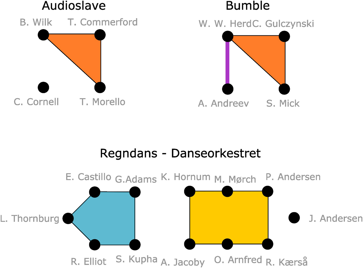
Illustration of the relationship between individual members of Audioslave, Bumble founders and musicians on recording of Regndans by Danseorkestret.
With the definition of m-patterns, and their instances in hypergraphs, we now have a formal way of talking about existing relationships between hypergraph vertices. In particular, when a new team of m individuals appears, we consider the team members’ past history of interactions to be the m-pattern consisting of all maximal subsets that have worked together before.
Definition 2.6Instance of a labelledm-pattern.An instance of a labelledm-patternXwith assigned vertex labels 1, 2, …, min the hypergraphis a maximal induced subhypergraphX′ onmnodes with assigned vertex labels 1, 2, … , mwhich is isomorphic toXand where corresponding vertices have the same assigned labels as inX.
In Supplementary Section S1, we illustrate connections between some of the concepts introduced in this section.
We are now ready to examine what m-patterns among nodes precede hyperedge formation in hypergraphs. In the following subsection, we will do so in a class of synthetic random hypergraphs.
2.2 G(m)(N, p) model of random hypergraphs
From Definition 2.4 and 2.5, it is clear that the structure of the underlying hypergraph greatly influences what m-patterns that can exist among sets of m nodes, and what multiplicity these m-patterns might have in the hypergraph. If the hypergraph is very sparse, most sets of m nodes have never collaborated before. For sparse hypergraphs, this presents us with the following question. When a newly formed team consists of m nodes with no past collaborations, is this because people tend to team up with strangers, or because the underlying hypergraph is sparse? If we want to understand whether some existing relationship structures are more likely to give rise to future team formations, we must know what to expect by chance alone. Studying m-patterns in a null-model of hypergraphs can help us gain intuition about what m-patterns we should expect to dominate at different hyperedge densities.
We choose to study m-patterns in a hypergraph generalization of the widely-studied random-graph family known as Erdős–Rényi graphs—or G(N, p). G(N, p) is known to create unrealistically simple graph structures. Nonetheless, the dyadic G(n, p) model has been a major driver in the development of the study of networks: it is the simplest random-graph model, analytically tractable, and its phenomena are correspondingly clear to articulate. We study a G(N, p)-type model for the same reasons.
In the classic G(N, p) model, an N-vertex random graph is created by inserting each possible edge with probability p [9]. Various hypergraph generalizations of the G(N, p) model have been studied in the past [36–40]. We choose to study a version where a hypergraph with N nodes and m-vertex hyperedges is created by inserting each possible hyperedge connecting m nodes with probability p. Since the parameters N, p and m define this hypergraph family, G(m)(N, p) is a natural name to summarize the family. The dyadic Erdős–Rényi graphs, normally known as G(N, p), would be G(2)(N, p) in this notation.
With the G(m)(N, p) model in hand, we set out to examine how often a new hyperedge would join m nodes with m-pattern X by chance, given that the hyperedge is forming in a hypergraph created using the G(m)(N, p) model with parameters N, p and m. To quantify this, we create a large number of G(m)(N, p) hypergraphs and count the average fraction of sets of m nodes that form each pattern X across these many random hypergraphs for choices of hypergraph size N, set size m and as a function of hyperedge probability p. In Figure 2, we show results obtained for two such simulations. In Figure 2A, the constructed hypergraphs have size N = 50 and contain hyperedges joining m = 3 nodes. In Figure 2B, the hypergraphs have size N = 100 and hyperedges join m = 4 nodes. The first thing to notice about these figures is that, when increasing p from 0, all but two m-patterns increase in prevalence, experience peak prevalence, and finally become less common again. The two patterns that do not take such journeys are: 1) the pattern in which noone collaborated with anyone before; and 2) the repeat collaboration. The occurrences of the no-past-collaboration pattern monotonically decreases with p, whereas the repeat-collaboration pattern increases monotonically with p. These “exceptions” are easily understood: As p increases, more nodes become part of m-node hyperedges. A higher p means that fewer nodes avoid collaborations altogether, whereas m-node collaborations (what we also call repeat collaborations) increase linearly with p.
FIGURE 2
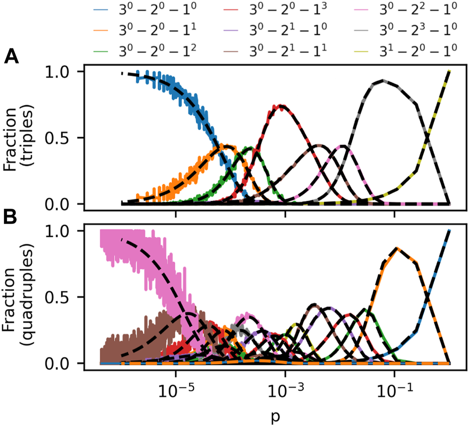
Frequency of m-patterns in the G(m)(N, p) model as a function of p for m = 3, N = 50 (A) and m = 4, N = 100 (B). Each datapoint is the average frequency of an m-pattern in 100 independent simulations of the model. The pattern 3i − 2j − 1k contains i 3-node, j 2-node and k 1-node hyperedges. Analytical estimates of prevalence in Eq. (1) is plotted with dashed lines. The legend above the figure panels describes the curves in (A). In (B), multiple curves are plotted with same colors; See Supplementary Section S2 for a labelled version of (B).
Having noticed regularities in the general shape of prevalence curves in Figure 2A, another interesting observation is that not all patterns get to be the most common for any p in Figure 2B. For example, the pattern consisting of a single 3-node hyperedge and a solitary node (dashed orange line) never outgrows all other patterns. This observation is interesting enough that we introduce a term for a pattern which gets to be the most common at a given value of p.
Definition 2.7Extreme pattern.Anm-pattern,X, is extreme if, for a particular value ofN, them-pattern is the most prevalent of allm-patterns for somep.
Definition 2.8Extreme in the limit.Anm-pattern,X, is extreme in the limit if there exists anN0such that for allN > N0there exists apwhere the pattern is the most prevalent of allm-patterns in the hypergraph.
A third interesting observation from Figure 2 is the order in which extreme patterns are the most common in the hypergraphs when increasing p. As p increases, the pattern with no previous collaborations is the most common at first. Then follow patterns containing disjoint nodes that all have previous collaborations, but none with each other. Then patterns that include dyadic collaborations, etc. These observations beg for explanations. Can we understand the shape of the prevalence curves and estimate them analytically? Can we understand which m-patterns are extreme and for which hyperedge densities, p, these patterns are the most common?
The answers to both of the above questions are yes. With the following theorem, we identify a sizeable number of patterns that cannot be extreme in the limit.
If the patternXcontainsH-node hyperedges and missesl + 1-node hyperedges, and |H − l|≥ 2,Xis not extreme in the limit.
Theorem 2.9 tells us why the m-pattern with a 3-node hyperedge and a solitary node is not extreme in Figure 2B (or rather, why it would not be in the limit N → ∞). The reason is that the pattern contains a 3-node hyperedge, and misses 2-node hyperedges that could have existed. Since |3 − (2 − 1)| = 2, Theorem 2.9 tells us that such a pattern cannot be extreme in the limit.
In order to prove Theorem 2.9, we will need 2 Lemmas. The first Lemma conveniently answers the second question we asked above: Can we understand the shape of the prevalence curves of m-patterns? We will answer this question by writing down a formula for the expected frequency of the m-pattern X among the instances of m-patterns in G(m)(N, p) hypergraphs. We can do this if we think about the prevalence of an m-pattern in the following way. The fraction of sets of m nodes that form an m-pattern X in a G(m)(N, p) hypergraph is equal to the probability that the pattern is formed by the m nodes when each size-m hyperedge is inserted with probability p. Calculating this probability is an exercise in combinatorics. The result reveals that the prevalence curve of any m-pattern takes the same analytical form.
Lemma 2.10LetXbe a pattern consisting ofxmm-node hyperedges,xm−1 (m − 1)-node hyperedges, … , andx1 1-node hyperedges. In addition, denote the number of missingi-node hyperedges byyi(xi, xi+1, … , xm). ForN ≥ mnodes and 0 ≤ p ≤ 1, the prevalence ofX, can be written,Here,is a combinatorial factor andpiis the probability thatinodes chosen uniformly at random from theNnodes, are connected by ani-simplex,where we defined.
The combinatorial factor γX counts the number of isomorphic configurations of X that exists on m nodes. Hence, the prevalence curve of a labelled version of m-patterns can be obtained by setting γX = 1. A side-effect of this fact is that all labelled versions of an m-pattern are equally likely under the G(m)(N, p) model.
Lemma 2.11For anyϵ > 0 and large enoughN, the values ofpat whichpl = a, for 0 < a < 1,pktake the values
ProofIf pl = a, Lemma 2.10 allows us to find the corresponding value of p,Inserting this in the formula for pk gives usNow let k > l. Then,Here we used the inequalityrepeatedly and defined β = (m − l)m−l/(m − k)! Taking the reciprocal value of both sides of Eq. (3) gives us the boundBecause 0 < (1 − a) < 1,What does N need to be larger than, if pk < ϵ? Demanding thatensures that pk < ϵ and allows us to isolate N,This proves half of the Lemma. For the other half, we now let k < l. With similar steps as in the previous case, we can get the bound,with β′ = (m − k)m−k/(m − l)! Taking the reciprocal value of both sides, the bound becomes,We now proceed in analogous manner as in the first half of the proof. With the bound on ck/cl,If this final quantity is larger than 1 − ϵ, pk is too. For what N is this the case then? Setting the final expression larger than 1 − ϵ and isolating N yieldsWe conclude that if N is larger than both of the values given in Eqs. (4) and (5),This proves the Lemma. With Lemmas 2.10 and 2.11, we now present our proof of Theorem 2.9.
Proof(Theorem 2.9) If the pattern X is extreme, all factors in the analytical expression for its prevalence must be large enough that P(X) takes a larger value than P (X′) for any other pattern X′. By Lemma 2.10, P(X) contains factors and , with yl+1, xH ≠ 0. By Lemma 2.11, if for some p, pH takes a value bounded away from 0 and 1, then one can choose an N large enough to make pk arbitrarily close to 1, if k ≤ H − 1. For any such k, (1 − pk) then becomes arbitrarily close to 0. Hence, if P(X) contains factors of both pH and (1 − pl+1), and |H − l|≥ 2, P(X) → 0 for large enough N, which implies it cannot be extreme in the limit.
Theorem 2.9 settles that a large class of m-patterns cannot be extreme in the limit. A natural next question to ask is then, what patterns are extreme in the limit? Are some types of patterns bound to be extreme? Are some types of patterns only extreme for certain choices of m?
Proving such positive results appears to be more challenging than proving the negative results of Theorem 2.9. A useful concept in proving such positive results is what we call a pure pattern.
Definition 2.12Pure pattern.Anm-pattern with no hyperedges other than all possiblek-node hyperedges is a pure pattern.
Pure patterns are easy to think about and work with because they contain only one kind of hyperedge, and there is only a single way of constructing each pure pattern. In Lemma 2.10, this means that γX = 1 for any pure pattern. The simplicity of working with pure patterns has caused these patterns to play a central role in our results on which patterns are actually extreme. One important result concerns exactly these pure patterns (proof given in Supplementary Section S3).
All pure patterns are extreme in the limit.
Our next theorem requires a result for labelled m-patterns. We remind the reader that instances of labelled m-patterns are different from instances of m-patterns in that we do not group isomorphic maximal induced subhypergraphs together. In this case, Lemma 2.10 still gives us the analytical expression for the prevalence of labelled m-patterns, but γ = 1 for all patterns.
The following two lemmas are proven in Supplementary Section S4, S5.
Lemma 2.14For labelledm-patterns andN → ∞, when, the pure pattern containing onlyk-node hyperedges is more frequent than all patterns consisting of bothk-node hyperedges and (k − 1)-node hyperedges.
Lemma 2.15For labelledm-patterns andN → ∞, when, the pure pattern containing onlyk-node hyperedges is more frequent than all patterns consisting of both (k + 1)-node hyperedges andk-node hyperedges.
These two Lemmas and Theorem 2.9 give us the following interesting result.
For labelledm-patterns, only pure patterns are extreme in the limit.
Moreover, the arguments leading to Lemmas 2.14 and 2.15 also lead us to the following Lemma (see also Supplementary Section S6),
Lemma 2.17For labelledm-patterns, all patterns consisting only of (k + 1)-node hyperedges and all possible remainingk-node hyperedges are equally prevalent when.
These results for labelled m-patterns help us prove the following more general theorem for non-labelled patterns.
Ifm ≥ 3 at least one non-pure pattern is extreme.
ProofIf m ≥ 3, non-pure patterns exist that do not violate Theorem 2.9. Since we are not dealing with labelled patterns, the combinatorial factor γ is some integer larger than or equal to 1 for each pattern. For pure patterns γX = 1. Now focus at the point . From Lemma 2.17, prevalence curves for several pure and non-pure labelled patterns cross at this point in the large-N limit. At least one of the corresponding non-labelled non-pure patterns has γX ≥ 2. For example, the pattern missing a single pm−1-node hyperedge and containing -node hyperedges instead has γX = m − 1. Hence, in this point, at least this non-pure pattern is more prevalent than the two pure patterns containing (m − 2)-node and (m − 1)-node hyperedges. For this reason, and Lemma 2.11, it is more prevalent than all pure patterns. This proves the Theorem.
Having shown that all pure patterns are extreme and that some none-pure patterns are extreme, too, we present a final result that shows that a large number of potentially extreme patterns are not extreme (proof in Supplementary Section S7).
Two differentm-patterns that have different combinatorial factors and consist only ofxkk-node hyperedges and all possible remaining (k − 1) hyperedges cannot both be extreme in the limit.
We note that in cases where several patterns compete for being extreme as described in Theorem 2.19, the pattern that actually gets to be extreme in the limit can have very different structure depending on m. The reason for this is that the combinatorial factor γ depends on the value of m. Take, for example, the two possible non-isomorphic patterns consisting of two two-node hyperedges and all remaining possible one-node hyperedges for m ≥ 4. In one pattern the two 2-node hyperedges share a node, whereas in the other, the 2-node hyperedges are completely separate. For a given choice of m, there are ways of constructing the m-pattern with linked 2-node hyperedges, and 3 ways of constructing the pattern with separate 2-node hyperedges. Hence, patterns with 2-node hyperedges in sequence have larger combinatorial factors when m ≤ 6, the patterns have the same combinatorial factor if m = 7 and patterns with parallel 2-node hyperedges dominate when m ≥ 8.
3 Hypergraph patterns in empirical data
The G(m)(N, p) model informs us how prevalent we should expect an m-pattern X to be in an N-node hypergraphs where a fraction p of possible m-node hyperedges exist if the hyperedges were distributed uniformly randomly among all possible m-node hyperedges. This raises a natural question: In empirical datasets, are some m-patterns overrepresented and others underrepresented compared to the G(m)(N, p) null-model?
3.1 Academic coauthorship hypergraphs
Making an informative comparison of m-patterns in empirical hypergraphs and the G(m)(N, p) model is not as straight forward as it sounds. Any empirical hypergraph has a fixed number of nodes and a given hyperedge density. For this reason, any comparison of the G(m)(N, p) model to an empirical hypergraph results in a comparison for just one value of p. Since one of the interesting features of the G(m)(N, p) model is how the prevalence of the m-patterns change with the hyperedge density p, we seek a large collection of hypergraphs with different hyperedge densities. We construct such a collection from the set of ego hypergraphs in empirical coauthorship hypergraphs. For each node v in the coauthorship hypergraph, , we construct an ego hypergraph . includes all neighbors of v, but not v itself. includes all m-node hyperedges between nodes in . Furthermore, for any m′-node hyperedge (m′ ≥ m + 1) in that joins m nodes from Ve and (m′ − m) nodes from , we include a subhyperedge in joining these nodes from .
Figure 3A shows the prevalence of 3-patterns in ego hypergraphs in a coauthorship hypergraph of scientists working in the field of Geology [6]. These ego hypergraph have very diverse hyperedge densities, p (horizontal axis). The ego hypergraphs also have different sizes, N. In the plot, we include results for all ego hypergraphs of sizes 10 ≤ N ≤ 50. Since the prevalence of m-patterns depends on N in the G(m)(N, p) model, the data points are not expected to fall on clear lines as were found for the null model. Indeed, instead of lines, datapoints for each pattern form point clouds in the Figure. This makes it difficult to compare the data to the model.
FIGURE 3
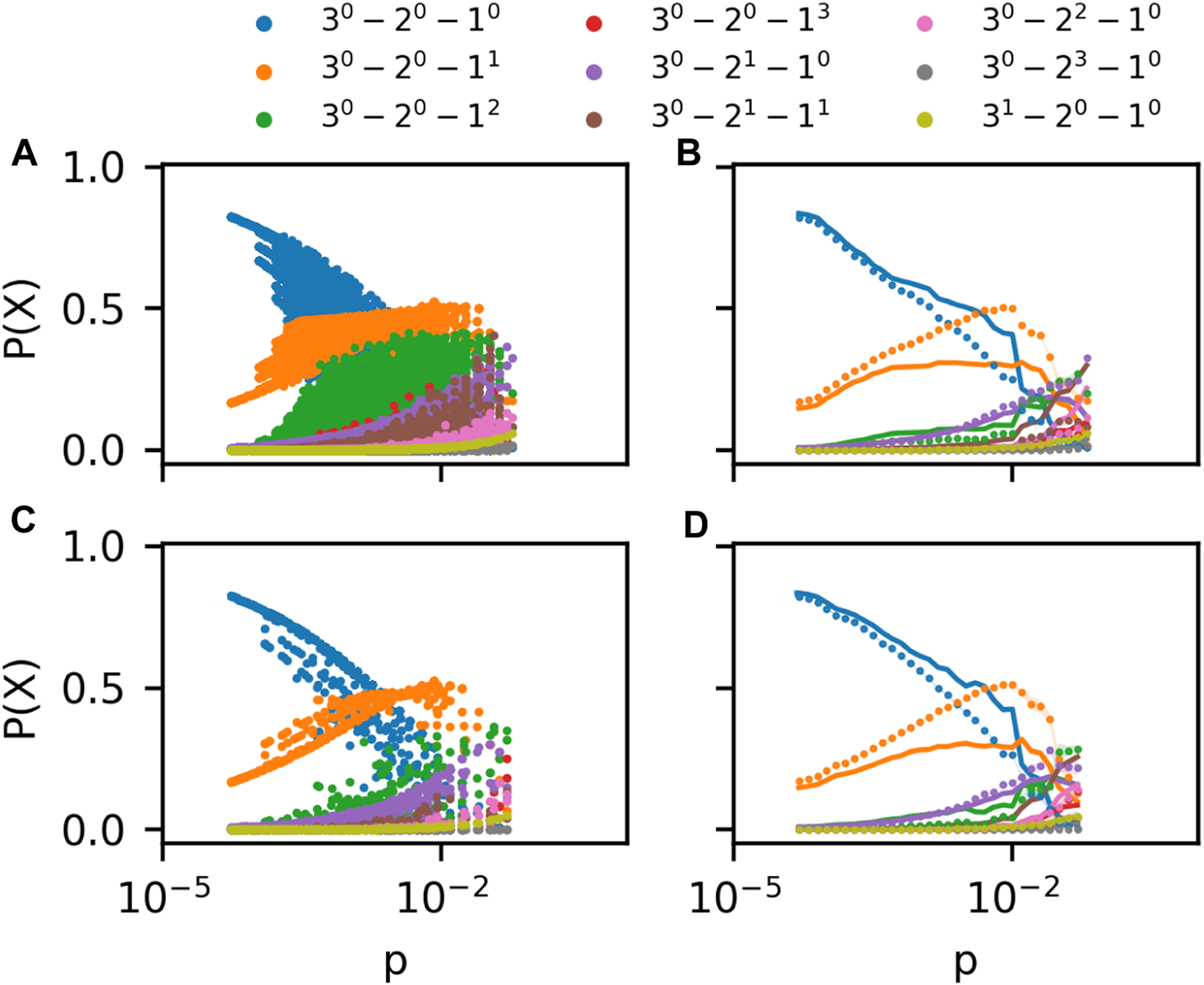
(A) Frequency of m-patterns in ego networks for sizes 10 ≤ N ≤ 50 in the Geology coauthorship network Benson et al. [6]. (B) Rolling average of data in (A) plotted alongside G(m)(N, p) prediction (curves) (C) As in (B) but for a History coauthorship network Benson et al. [6] (D) As in (B). In all panels, colors indicate the m-pattern shown in the legend.
In Figure 3B, we show the same data after performing a rolling average. In this panel we split the logarithmic horizontal axis into equidistant segments; 10 for each order of magnitude. For each segment, we calculate an average prevalence of all 3-patterns X. Every datapoint with p-value between the p-values of segments i − 1 and i + 1 count in the average calculated for segment i. The data is plotted with dots. The G(m)(N, p) expectation (curves) was created by plugging the empirical values for N and p for each ego hypergraph into the G(m)(N, p) model. We then performed our averaging procedure to the resulting point cloud.
Although there are similarities between prevalence curves of 3-patterns in the empirical ego hypergraphs and the model, there are clear discrepancies as well. For example, the pattern with just a single 1-hyperedge is clearly overrepresented in the data for several orders of magnitude of the hyperedge density p. On the other hand, the pattern consisting of a 1-node and a 2-node hyperedge is underrepresented in the data. Similar plots of a dataset of coauthorships in the field of history confirms these observations (Figures 3C, D).
3.2 Hypergraphs of human and non-human systems
The similarity of Figures 3B, D is striking. For the two different coauthorship hypergraphs, many of the same patterns seem to be underrepresented and overrepresented as compared to the G(m)(N, p) null model. The two datasets both stem from academic coauthorship hypergraphs. Could the similarities in m-pattern prevalence be due to the fact that the hypergraphs stem from the same domain? And if so, which patterns are overrepresented or underrepresented in hypergraphs from other domains?
In Figure 4 we compare the prevalence of m-patterns in ego hypergraphs of 9 different empirical hypergraphs to the G(N, p) model. The hypergraphs represent very different domains: Human and non-human, processes on the web and in nature. Hypergraphs represent email networks (“Enron”), drug networks (“NDC-classes” and “NDC-substances”), human contact networks (“contact-primary-school” and “contact-high-school”), online tagging data (“tags-math-sx” and “tags-ask-ubuntu”) and the academic coauthorship networks introduced above. The vertical axes quantify the difference between the prevalence of m-patterns in the empirical ego hypergraphs and the G(N, p) model, Δf = [P (Xdata) − P (Xmodel)]/min (P (Xmodel), P (Xdata)). The color and shape of the marker depends on the domain that the ego hypergraph represents.
FIGURE 4
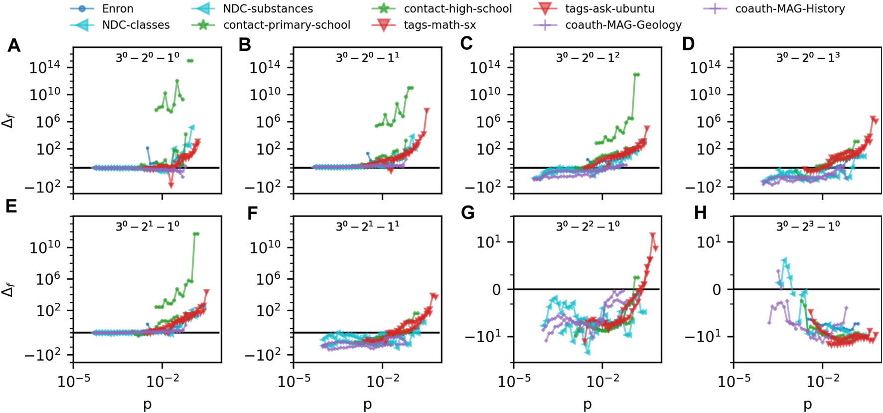
(A–H) quantify the difference between m-pattern prevalence in 9 datasets as compared to our G(m)(N, p) model. The difference measure is Δf = [P (Xdata) − P (Xmodel)]/min (P (Xmodel), P (Xdata)) and Δf = 0 corresponds to perfect agreement between data and model. Each panel plots Δf for a specific 3-pattern as found in all 9 datasets.
The first thing to notice in Figure 4 is how numerically large the values on the vertical axes are (note the symmetrical logarithmic axes). If a datapoint is plotted at vertical value 10, the pattern is 10 times more prevalent in the data than in the model. So with the vertical scale covering the interval [−102, 1014], some patterns are vastly over and underrepresented in the data.
A second thing to notice in Figure 4 is that some patterns are consequently underrepresented in data. Most clearly underrepresented is the pure pattern of 2-node hyperedges (Figure 4H). For all datasets but “NDC-classes” this lies clearly in the negative vertical values. The pattern consisting of a 2-node and 1-node hyperedge and the pattern with just 2 2-node hyperedges (Figures 4F, G) are also mostly underrepresented in the datasets.
A third and interesting aspect of Figure 4 is hints of similarities between datasets from similar domains. With the exception of the school contact networks, datapoints from similar domains fall very close together on the plots.
Figure 4 represents one way of comparing prevalence of m-patterns for different datasets. In Figure 5 we provide another. Each panel in the figure shows a scatter plot of the prevalence of 3 3-patterns in each of the empirical ego hypergraphs. The color and shape of the marker depends on the domain that the ego hypergraph represents. We also plot the results for our G(m)(N, p) model (with N = 50). In all panels, the model traces out a parametric curve starting in the point marked by a black dot. Interestingly, the data are not scattered all around the curve; instead, for these scatter plots, datapoints often fall in a limited subspace around the curve. While we have no theoretical explanation for this tendency for data to cluster in a limited subspace around the curve, we believe that the tendency might be explained by studying how the frequency of different m-patterns are correlated. We also note that Ugander et al. derived bounds for subgraph frequencies in a system related to ours–frequencies of induced subgraphs in larger graphs [41]—and that extending these methods might cast further light on the matter. Lastly, the panels show that datapoints from similar domains fall close together. We note that some of this separation could be due to the different orders of magnitude of the hyperedge densities, p, present in each dataset (see Figure 4).
FIGURE 5
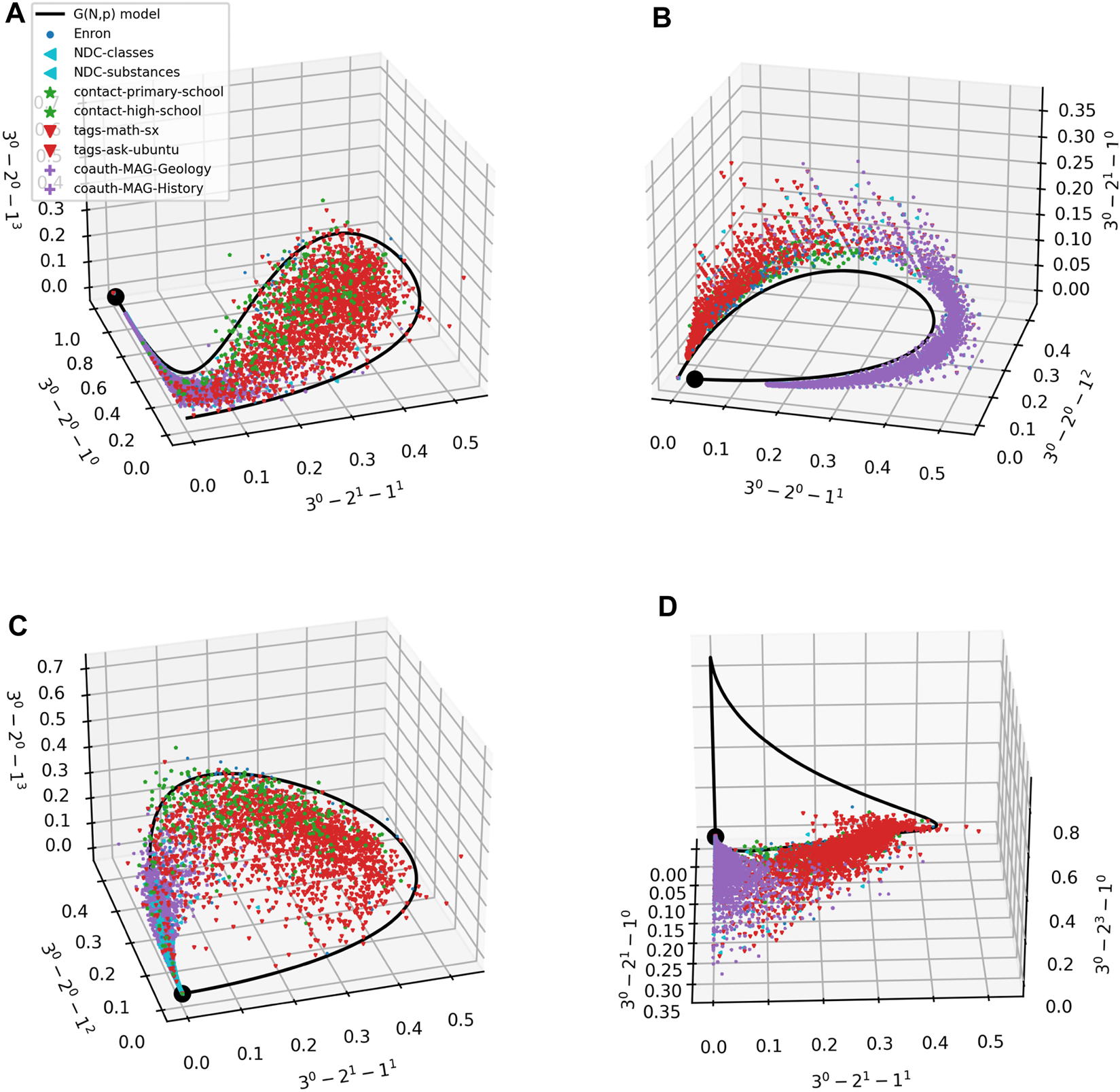
(A–D) Scatter plots of ego networks in 9 empirical datasets. Markers as in Figure 4. Each axis is a 3-pattern; axes are different in panels. The G(m)(N, p) model traces out the black curves; the black dot corresponds to the lowest hyperedge density p on the curve.
4 COVID-19 collaborations
In the previous 2 sections, we have counted the prevalence of m-patterns in empirical ego hypergraphs and our G(m)(N, p) model. The hypergraphs we were examining were always fully grown. One of our main motivations for introducing m-patterns was to investigate what prior relationships between a set of m nodes are likely to exist when these nodes choose to collaborate. To confront this question, we now examine hyperedge formation in a growing hypergraph: the coauthorship network of papers submitted to the arxiv.org, biorxiv.org and medrxiv.org preprint servers.
Figures 6A, C show what fraction of authors on new 2-author and 3-author papers had prior relationships that could be summarized by different m-patterns. The curves are shown as a function of time; time running from the first datapoints for arxiv.org and until 1 September 2020. Datapoints are averages of all papers uploaded in a given month. As the coauthorship hypergraph grows, the likelihood of different prior relationship structures leading to a new m-author paper changes. We speculate that each of these curves converges to some value with time. For both 3 and 2-author preprints, the repeat collaboration is the most frequent collaboration structure in 2020.
FIGURE 6
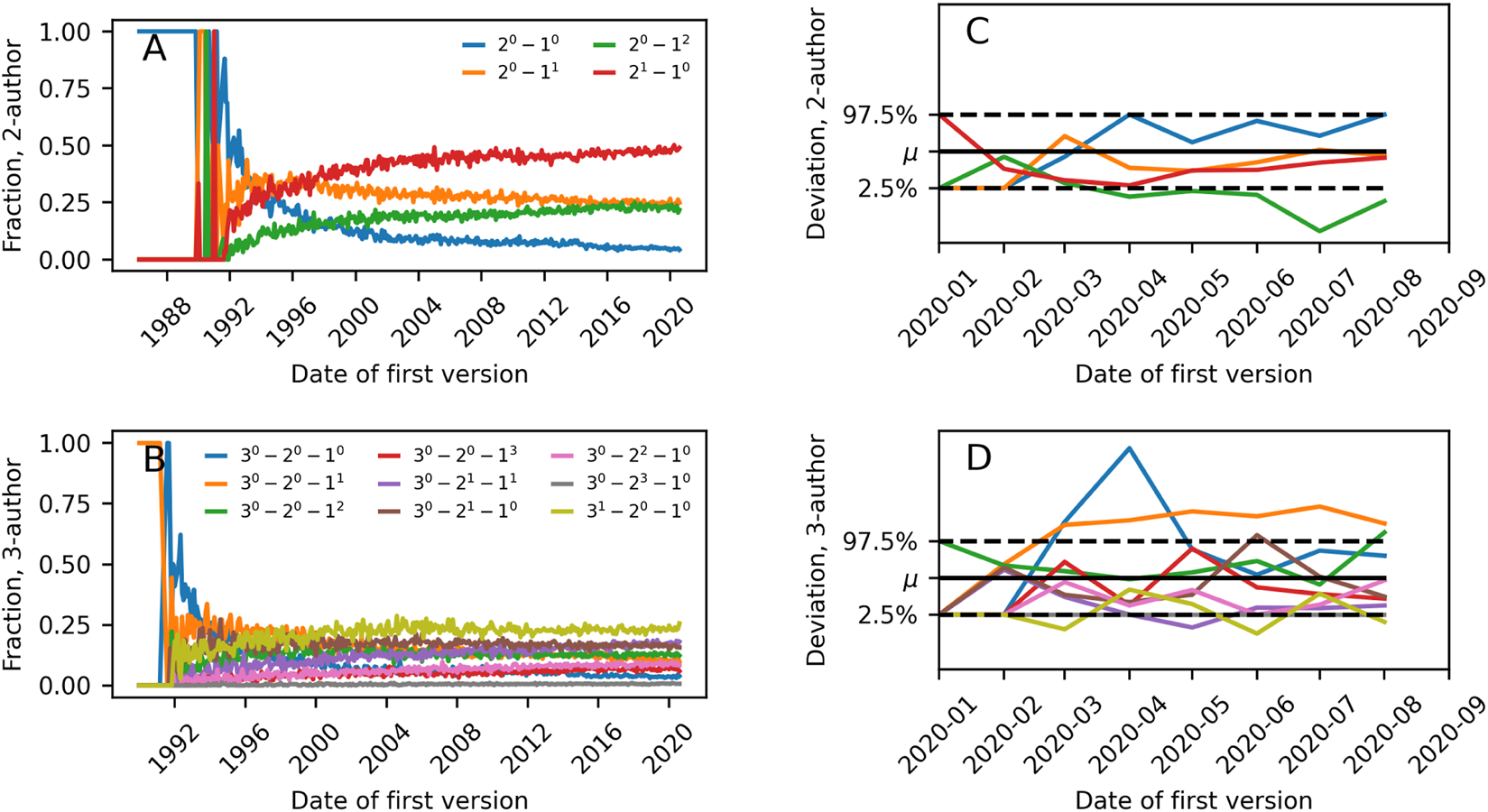
(A) Frequency of 2-patterns for new collaborations in scientific preprints (on arXiv.org, biorxiv.org and medrxiv.org) as a function of time. (B) as in (A) but for 3-patterns. (C) Illustration of deviation of m-pattern frequency among collaborating scientists on early COVID-19 papers as compared to expectation from the general body of preprints. μ indicates expectation and dashed lines the 2.5 and 97.5 percentiles. (D) as in (C) but for 3-patterns.
During the spring of 2020, a surge of COVID-19 related papers accompanied the rising pandemic. Teams working on early COVID-19 papers must have formed quickly, and worked intensively to analyze the disease and its consequences. Keeping the common collaboration structures found in Figures 6A, C in mind, one might wonder whether collaboration structures looked different for these papers that were induced by the external shock of the pandemic. For example, related previous work has established that for a particular subset of these papers–multidisciplinary COVID-19 papers–collaborations were smaller and more diverse than other collaborations [42].
Figures 6B, D compare the collaboration structure of COVID-19 papers in our dataset to the collaboration structure frequencies found in the entire dataset (COVID-19 papers defined as papers with at least one of the following words in the abstract: covid, covid19, covid-19, sars-cov-2, sars-cov2). If ni COVID-19 papers were uploaded in month i, we compare the frequency of the pattern X to how often we would obtain that pattern when drawing ni preprints uniformly randomly from all preprints in month i. In the data there are significant differences in collaboration structure of COVID-19 papers released between January and August 2020 as compared to papers on all topics in the same period. For 2-author papers, collaborations between two scientists with prior publications but no past joint papers happen less than expected. For 3-author papers, we find more collaborations consisting of two newcomers and a scientist with prior publications than expected.
5 Relation between team structure and citation count
A question that has attracted considerable attention in the literature, is whether team structure influences team performance [1–4]; [43]. Previous studies have examined correlations between performance of teams and team size or dyadic team network structure. Here, we investigate the relation between higher-order team structure—in the form of m-patterns—in scientific collaborations and team performance (crudely estimated as the number of citations of published work).
We study scientific collaborations and their success using the Open Academic Graph (MAG) data set (version 1) [44, 45]. The dataset contains more than 166 million papers including information such as author names, affiliations, publication year, number of citations at the time of data collection, field of study (in the form of keywords) and more.
To assess whether team structure might affect team performance, it is necessary to consider a number of other variables that could influence how many citations a publication receives. For example, citations could depend on the field of study, the age of the paper, whether the authors on the publication publish in the field often or rarely, and whether they generally receive many citations on their publications.
To control for the factors other than team structure that could influence citation count, we analyze the data as follows. First, we only compare citation counts for papers within the same field of study. We examine papers from 4 fields of study: Computer Science, Geology, Mathematics and Sociology. We gather papers from each field of study in separate data sets including only papers where the field of interest is a keyword in the paper’s MAG “field of study” data. For each of the 4 fields, we construct an academic collaboration network from the gathered papers and determine the m-pattern collaboration structure of each paper. Second, to resolve whether citations are correlated to team structure or other variables, we use a linear regression model to predict the number of citations of a paper based on other variables that could influence citation count: Paper age, mean number of citations of paper authors, mean number of publications of paper authors, and the mean time since paper authors published their first paper. We train the model on 80% of a dataset that is balanced such that it contains equally many papers with the team structures under consideration (we focus on 2 kinds of team structures: repeat collaborations and first-time collaborations with no first-time authors), and such that these two sets of papers have identical age distributions (for two sets of papers A and B, each with A(y) and B(y) papers of age y, we create two subsampled datasets with identical age distributions, and ; these include min (A(y), B(y)) published in year y from A and B, respectively, drawing papers uniformly at random without replacement from the original sets). For the remaining 20% of papers, we compute the deviation between citations as predicted by the model and actual citations. We quantify this deviation as a mean fractional error of the citation prediction xpredicted to the actual citation number xactual,where we set i = 1 for first-time collaborations and i = 2 for repeat collaborations. Finally, we evaluate to what degree the model underestimated citation count of repeat collaborations compared to first-time collaborations or vice versa by performing two-sample tests for these summary statistics.
Table 1 shows our results for 2-author and 3-author papers. For Computer Science, 2-author repeat collaborations get more citations than would be expected from the trained model alone; moreover, the 2-author repeat collaborations outperform model expectations to a statistical significant higher degree than is done by 2-author first-time collaborations. For 3-author Computer Science collaborations the result is the opposite: 3-author first-time collaborations outperform the model prediction to a statistically significant level compared to the repeat collaboration. The findings for 2-author papers in Geology and 3-author papers in mathematics mimic those found for computer science: 2-author repeat Geology collaborations and 3-author first-time mathematics collaborations both get statistically significantly more citations than expected from the model that assumes that collaboration structure does not correlate with citation numbers. For the remaining collaborations (3-author Geology papers, 2-author mathematics papers and both 2-author and 3-author sociology papers) citations do not deviate to a statistical significant degree for new collaborations and repeat collaborations.
TABLE 1
| Field | Team size | z-score | ||
|---|---|---|---|---|
| Computer Science | 2 authors | 0.3521 ± 0.0043 | 0.3690 ± 0.0046 | 2.670 |
| 3 authors | 0.3818 ± 0.0055 | 0.3554 ± 0.0058 | 3.304 | |
| Geology | 2 authors | 0.2342 ± 0.0055 | 0.2571 ± 0.0064 | 2.717 |
| 3 authors | 0.1377 ± 0.0050 | 0.1369 ± 0.0049 | 0.102 | |
| Mathematics | 2 authors | 0.2155 ± 0.0039 | 0.2199 ± 0.0042 | 0.762 |
| 3 authors | 0.2846 ± 0.0052 | 0.2697 ± 0.0050 | 2.055 | |
| Sociology | 2 authors | 0.3184 ± 0.0179 | 0.2908 ± 0.0145 | 1.200 |
| 3 authors | 0.2164 ± 0.0178 | 0.2016 ± 0.0179 | 0.585 |
Relationship between past collaborations and future citations of academic papers in 4 different scientific fields.
For each field, we make two comparisons. In the first, we compare citations of 2-author papers where both authors have published in the past, but never together (the 2-pattern 20 − 12), to citations of 2-author papers where the authors have collaborated with each other in the past (the 2-pattern 21 − 10). In the second comparison, we compare citations of 3-author papers where all authors have published in the past but never all three together (the union of the 3-patterns 30 − 20 − 13, 30 − 21 − 11, 30 − 22 − 10 and 30 − 23 − 10) to citations of 3-author papers where the triple of authors is a repeat collaboration (the 3-pattern 31 − 20 − 10). We train a linear regression to predict citation count from the 4 properties of a paper: paper age, mean number of past publications of the authors, mean number of citations of the authors, and mean time since the authors published their first papers. μ1 indicates the mean error (see main text) on citation predictions for first-time collaborations and μ2 the mean error on predictions for repeat collaborations. Lastly, we estimate whether these mean fractional errors are significantly different from each other by computing the z-score of the pairs of estimates.
6 Discussion
In many different contexts, individual nodes occasionally co-occur together. Understanding which nodes are likely to form such collaborations, and how prior relationships influence collaboration outcome is important to study. In this work, we have introduced the concept of m-patterns, a new family of structural patterns that quantify prior relationships between m nodes in a hypergraph.
We have argued that prevalence of different such m-patterns should depend on hypergraph characteristics such as density of hyperedges, and we have quantified these expectations by studying a G(m)(N, p) model. In particular, we have derived analytical expressions for m-pattern prevalence and provided proofs that some patterns are and others can never be extreme in the G(m)(N, p) model in the limit N → ∞.
Comparing the model to data from different domains, we found both similarities and differences. Most strikingly, we found that some datasets had certain patterns overrepresented by several orders of magnitude as compared to the model expectation. Interestingly, datasets from the same domain often had similar discrepancies as compared to the model.
In the dataset of preprints, we found the repeat collaboration to be the most prevalent for both 2-author and 3-author papers. This is interesting because such a finding would only take place in very dense networks if collaborations were happening uniformly randomly. We proceeded to examine whether collaboration structure was different for early COVID-19 preprints as compared to the full dataset of preprints. We found that 2-author papers were less often coauthored by two scientists with prior publications but no collaborations. For 3-author preprints, we found more collaborations structures consisting of two newcomers and a person with previous publications.
Finally, we examined whether team structure of academic papers correlated with future citation counts. Considering 2-author and 3-author publications separately, we compared citations of first-time collaboration without first-time authors to citations of repeat collaborations in the fields of Computer Science, Geology, Mathematics and Sociology. Controlling for several factors, we trained a linear regression model to predict future citation counts based on paper and author details. For 2-author papers, we found that repeat collaborations outperformed model expectations in the fields of Computer Science and Geology. For 3-author papers on the other hand, new collaborations outperformed model expectations for Computer Science and Mathematics. The linear model is crude and for all fields it tended to underestimate citation count by between 13% and 39% of the actual future citation counts. This being said, the consistency of the statistically significant results speak to their trustworthiness: We found that repeat collaborations had better performance for 2-author collaborations whereas first-time collaborations had better performance for 3-author collaborations.
There are several natural future research directions related to our work.
In our modeling efforts, we have focused our attention on a random-hypergraph family related to the class of random graphs known as G(N, p). The simplicity of this hypergraph family allowed us to make a range of theoretical contributions. Nonetheless, there are many graph families that resemble empirical networks more in various aspects than the G(m)(N, p) model does. In future work, it would be natural to study m-patterns and their prevalence in the higher-order network extensions of the configuration model [9]; [27], exponential random graph models [27], and growing networks such as the scale-free Barabási-Albert preferential-attachment model [46] and the CHKNS uniform-attachment model [47] To extend our analytical results on m-patterns to a larger class of models from the rich back catalogue of network models, future work must adjust Eq. (2) in Lemma 2.10 to depend on other variables than the variables N and p that are specific to the G(m)(N, p) model studied here. We anticipate that many of the results related to pattern extremity will depend on family of random hypergraphs in question.
Throughout this paper, we have argued that investigating whether team structure correlates with team performance is an interesting question. Although we did examine this for 2-author and 3-author papers from 4 fields, there are many promising questions in this direction. We found different results for 2-author and 3-author papers; what happens for larger collaborations? And if repeat collaborations tend to have higher or lower performance, is the effect larger, smaller or unchanged for teams that collaborate over and over again? Our investigation of whether datasets from the same domains tend to have the same m-patterns over and underrepresented remains qualitative. An obvious next step would be to attempt to train an algorithm to guess the domain that a hypergraph stems from given only information about m-pattern prevalence. We note that such investigations should carefully control for the fact that data from different domains typically cover different orders of magnitudes of the hyperedge density p. Finally, we note that collaboration hypergraphs such as the preprint coauthorship network are growing systems. Although models for collaboration networks exist [2], these are based on dyadic interactions. Formulating a growth model that gives rise to correct m-pattern frequencies is an open question.
Statements
Data availability statement
Publicly available datasets were analyzed in this study. This data can be found here: https://www.cs.cornell.edu/∼arb/data/, https://github.com/jonassjuul/m-patterns.
Author contributions
JJ: Conceptualization, Data curation, Formal Analysis, Investigation, Methodology, Writing–original draft, Writing–review and editing. AB: Conceptualization, Investigation, Methodology, Supervision, Writing–review and editing. JK: Conceptualization, Investigation, Methodology, Supervision, Writing–review and editing.
Funding
The author(s) declare financial support was received for the research, authorship, and/or publication of this article. JJ’s work presented here is supported by the Carlsberg Foundation, grant CF21-0342. JK’s work was supported in part by a Vannevar Bush Faculty Fellowship, AFOSR grant FA9550-19-1-0183, a Simons Collaboration grant, and a grant from the MacArthur Foundation.
Conflict of interest
The authors declare that the research was conducted in the absence of any commercial or financial relationships that could be construed as a potential conflict of interest.
Publisher’s note
All claims expressed in this article are solely those of the authors and do not necessarily represent those of their affiliated organizations, or those of the publisher, the editors and the reviewers. Any product that may be evaluated in this article, or claim that may be made by its manufacturer, is not guaranteed or endorsed by the publisher.
Supplementary material
The Supplementary Material for this article can be found online at: https://www.frontiersin.org/articles/10.3389/fphy.2023.1301994/full#supplementary-material
References
1.
NielsenM. Reinventing Discovery: the new era of networked science. New Jersey, United States: Princeton University Press (2013).
2.
GuimeraRUzziBSpiroJAmaralLAN. Team assembly mechanisms determine collaboration network structure and team performance. Science (2005) 308:697–702. 10.1126/science.1106340
3.
WuLWangDEvansJA. Large teams develop and small teams disrupt science and technology. Nature (2019) 566:378–82. 10.1038/s41586-019-0941-9
4.
TrösterCMehraAvan KnippenbergD. enStructuring for team success: the interactive effects of network structure and cultural diversity on team potency and performance. Organizational Behav Hum Decis Process (2014) 124:245–55. 10.1016/j.obhdp.2014.04.003
5.
BensonARGleichDFLeskovecJ. Higher-order organization of complex networks. Science (2016) 353:163–6. 10.1126/science.aad9029
6.
BensonARAbebeRSchaubMTJadbabaieAKleinbergJ. Simplicial closure and higher-order link prediction. Proc Natl Acad Sci (2018) 115:E11221-E11230–E11230. 10.1073/pnas.1800683115
7.
BattistonFCencettiGIacopiniILatoraVLucasMPataniaAet alNetworks beyond pairwise interactions: structure and dynamics. Phys Rep (2020) 874:1–92. 10.1016/j.physrep.2020.05.004
8.
BensonARGleichDRHighamDJ. En-USHigher-order network Analysis takes off, fueled by old ideas and new data (2021).
9.
NewmanMEJ. Networks. 2. Oxford, United Kingdom ; New York, NY: United States of America: Oxford University Press (2018).
10.
JacksonMO. engSocial and economic networks. Princeton, NJ: Princeton Univ. Press (2008). OCLC: 254984264.
11.
EasleyDKleinbergJ. Networks, crowds, and markets: reasoning about a highly connected world. New York: Cambridge University Press (2010). OCLC: ocn495616815.
12.
KamińskiBPoulinVPrałatPSzufelPThébergeF. Clustering via hypergraph modularity. PLOS ONE (2019) 14:e0224307. 10.1371/journal.pone.0224307
13.
KumarTVaidyanathanSAnanthapadmanabhanHParthasarathySRavindranB. Hypergraph clustering by iteratively reweighted modularity maximization. Appl Netw Sci (2020) 5:52. 10.1007/s41109-020-00300-3
14.
ChodrowPSVeldtNBensonAR. Generative hypergraph clustering: from blockmodels to modularity. Science Advances (2021) 7 (28): eabh1303. 10.1126/sciadv.abh1303
15.
YinHBensonARLeskovecJGleichDF. enLocal higher-order graph clustering. In: Proceedings of the 23rd ACM SIGKDD International Conference on Knowledge Discovery and Data Mining (Halifax NS Canada: ACM) (2017). p. 555–64. 10.1145/3097983.3098069
16.
YinHBensonARLeskovecJ. Higher-order clustering in networks. Phys Rev E (2018) 97:052306. 10.1103/PhysRevE.97.052306
17.
BensonARGleichDFLeskovecJ. Tensor spectral clustering for partitioning higher-order network structures. In: Proceedings of the 2015 SIAM International Conference on Data Mining (SDM) (Society for Industrial and Applied Mathematics), Proceedings; 11-13 February 2020; Seattle, Washington, USA (2015). p. 118–26. 10.1137/1.9781611974010.14
18.
ChienILinC-YWangI-H. enCommunity detection in hypergraphs: optimal statistical limit and efficient algorithms. In: International Conference on Artificial Intelligence and Statistics (PMLR); 9 April 2018; Lanzarote, Canary Islands (2018). p. 871–9.
19.
AhnKLeeKSuhC. Hypergraph spectral clustering in the weighted stochastic block model. IEEE J Selected Top Signal Process (2018) 12:959–74. 10.1109/JSTSP.2018.2837638
20.
VeldtNBensonARKleinbergJ. Combinatorial characterizations and impossibilities for higher-order homophily. Science Advances (2023) 9 (1): eabq3200. 10.1126/sciadv.abq3200
21.
LandryNWRestrepoJG. Hypergraph assortativity: a dynamical systems perspective. Chaos: Interdiscip J Nonlinear Sci (2022) 32:053113. 10.1063/5.0086905
22.
LeeGKoJShinK. Hypergraph motifs: concepts, algorithms, and discoveries. Proc VLDB Endowment (2020) 13:2256–69. 10.14778/3407790.3407823
23.
KookYKoJShinK. ”Evolution of real-world hypergraphs: patterns and models without oracles,” in 2020 IEEE International Conference on Data Mining (ICDM). IEEE (2020).
24.
CourtneyOTBianconiG. Generalized network structures: the configuration model and the canonical ensemble of simplicial complexes. Phys Rev E (2016) 93:062311. 10.1103/physreve.93.062311
25.
CourtneyOTBianconiG. Weighted growing simplicial complexes. Phys Rev E (2017) 95:062301. 10.1103/physreve.95.062301
26.
BianconiGRahmedeC. Emergent hyperbolic network geometry. Scientific Rep (2017) 7:41974–9. 10.1038/srep41974
27.
YoungJ-GPetriGVaccarinoFPataniaA. Construction of and efficient sampling from the simplicial configuration model. Phys Rev E (2017) 96:032312. 10.1103/PhysRevE.96.032312
28.
KimCBandeiraASGoemansMX. Stochastic block model for hypergraphs: statistical limits and a semidefinite programming approach (2018). Available at: https://arxiv.org/abs/1807.02884 (Accessed December 22, 2023).
29.
ChodrowPS. Configuration models of random hypergraphs. J Complex Networks (2020) 8. 10.1093/comnet/cnaa018
30.
DyerMGreenhillCKleerPRossJStougieL. Sampling hypergraphs with given degrees. Discrete Mathematics (2021) 344 (11): 112566.
31.
BattistonFAmicoEBarratABianconiGFerraz de ArrudaGFranceschielloBet alThe physics of higher-order interactions in complex systems. Nat Phys (2021) 17:1093–8. 10.1038/s41567-021-01371-4
32.
YoungJ-GPetriGPeixotoTP. Hypergraph reconstruction from network data. Communications Physics (2021) 4 (1): 135.
33.
LeeGChoeMShinK. How do hyperedges overlap in real-world hypergraphs? - patterns, measures, and generators. In: Proceedings of the Web Conference 2021 (Ljubljana, Slovenia: Association for Computing Machinery), WWW ’21; April 19-23 2021; New York; NY (2021). p. 3396–407. 10.1145/3442381.3450010
34.
BrettoA. Hypergraph theory. An introduction. mathematical engineering. Cham: Springer (2013).
35.
BergeC. Hypergraphs: combinatorics of finite sets, vol. 45. Amsterdam, Netherlands: Elsevier (1989).
36.
LinialNMeshulamR. Homological connectivity of random 2-complexes. Combinatorica (2006) 26:475–87. 10.1007/978-3-319-00080-0
37.
MeshulamRWallachN. Homological connectivity of random k-dimensional complexes. Random Structures and Algorithms (2009) 34:408–17. 10.1002/rsa.20238
38.
CostaAFarberM. Random simplicial complexes. In: Configuration spaces. Cham: Springer (2016). p. 129–53.
39.
KahleM. Topology of random clique complexes. Discrete Math (2009) 309:1658–71. 10.1016/j.disc.2008.02.037
40.
KahleM.Topology of random simplicial complexes: a survey. AMS Contemp Math (2014) 620:201–22. 10.1090/conm/620/12367
41.
UganderJBackstromLKleinbergJ.Subgraph frequencies: mapping the empirical and extremal geography of large graph collections. In: Proceedings of the 22nd international conference on World Wide Web (2013). p. 1307–1318. 10.1145/2488388.2488502
42.
CunninghamESmythBGreeneD. Collaboration in the time of covid: a scientometric analysis of multidisciplinary sars-cov-2 research. Humanities Soc Sci Commun (2021) 8:240–8. 10.1057/s41599-021-00922-7
43.
ZengAFanYDiZWangYHavlinS. Fresh teams are associated with original and multidisciplinary research. Nat Hum Behav (2021) 5:1314–22. 10.1038/s41562-021-01084-x
44.
TangJZhangJYaoLLiJZhangLSuZ. Arnetminer: extraction and mining of academic social networks. In: Proceedings of the 14th ACM SIGKDD international conference on Knowledge discovery and data mining (2008). p. 990–8.
45.
SinhaAShenZSongYMaHEideDHsuB-Jet alAn overview of microsoft academic service (mas) and applications. In: Proceedings of the 24th international conference on world wide web (2015). p. 243–6.
46.
BarabásiALAlbertR. Emergence of scaling in random networks. Science (1999) 286 (5439):509–512.
47.
CallawayDSHopcroftJEKleinbergJMNewmanMEStrogatzSH. Are randomly grown graphs really random?. Physical Review E (2001) 64 (4):041902.
Summary
Keywords
hypergraphs, team performance, collaboration structure, COVID-19, motifs, random graphs
Citation
Juul JL, Benson AR and Kleinberg J (2024) Hypergraph patterns and collaboration structure. Front. Phys. 11:1301994. doi: 10.3389/fphy.2023.1301994
Received
25 September 2023
Accepted
13 December 2023
Published
11 January 2024
Volume
11 - 2023
Edited by
Ingo Scholtes, Julius Maximilian University of Würzburg, Germany
Reviewed by
Roberta Sinatra, IT University of Copenhagen, Denmark
Chaoming Song, University of Miami, United States
Updates
Copyright
© 2024 Juul, Benson and Kleinberg.
This is an open-access article distributed under the terms of the Creative Commons Attribution License (CC BY). The use, distribution or reproduction in other forums is permitted, provided the original author(s) and the copyright owner(s) are credited and that the original publication in this journal is cited, in accordance with accepted academic practice. No use, distribution or reproduction is permitted which does not comply with these terms.
*Correspondence: Jonas L. Juul, jlju@dtu.dk
Disclaimer
All claims expressed in this article are solely those of the authors and do not necessarily represent those of their affiliated organizations, or those of the publisher, the editors and the reviewers. Any product that may be evaluated in this article or claim that may be made by its manufacturer is not guaranteed or endorsed by the publisher.