Tripartite Svetlichny test with measurement dependence

1 Introduction

Quantum nonlocality is a critical resource in device-independent quantum information processing tasks such as quantum key distribution [1–3], random number generation [4–7], self-testing [8,9], and private query [10,11]. The phenomenon of quantum nonlocality, first brought to light in the famous debate between Einstein, Podolsky, and Rosen in 1935 [12], was later given a testable framework by Bell through his inequality theorem formulated in 1964 [13].

A bipartite Bell test involves two distant parties: Alice and Bob. Each party randomly selects measurement settings A_x(x ∈ {0, 1}) and B_y(y ∈ {0, 1}) and obtains outcomes a ∈ {0, 1} and b ∈ {0, 1}, respectively. After many rounds of experiments, the statistical correlations are characterized by the joint probability distribution p(a, b|A_x, B_y). Bell inequality can be defined by a linear combination of p(a, b|A_x, B_y):

$\langle A_0{B}_0\rangle +\langle A_0{B}_1\rangle +\langle A_1{B}_0\rangle -\langle A_1{B}_1\rangle \le 2,(1)$

where ⟨A_xB_y⟩ = ∑_a,b(−1)^a+bp(a, b|A_x, B_y). This inequality is known as the CHSH inequality [14]. The statistical correlations produced by the classical system can reach the local upper bound of CHSH inequality of 2. In quantum mechanics, measurements acting on quantum entanglement states can violate the CHSH inequality and result in a bound value of up to $2\sqrt{2}$.

Since the 1980s, Bell test experiments have been realized [15–18], but it has been found that these experiments suffer a loophole called randomness loophole. The Bell test requires that the selection of measurements is completely random. This is a basic assumption for the Bell test, called measurement independence. If measurement independence cannot be guaranteed in the experiment, the randomness loophole will be opened up. The adversary Eve is able to simulate quantum nonlocality with classical systems by possessing a priori knowledge of measurement settings, which threatens the security of device-independent quantum information processing tasks. Nevertheless, measurement independence is difficult to be guaranteed in practical Bell tests. Many researchers have attempted to explore how relaxing the measurement independence assumption (i.e., measurement dependence) would affect the Bell test [19–30].

In 2010, Hall [19] proposed the quantification of measurement dependence and constructed a local deterministic model to simulate singlet state correlations. In 2012, Koh et al. [21] explored the effects of measurement dependence on the CHSH–Bell test. By considering the relation among measurement dependence, guessing probability, and the maximal value of CHSH inequality, they bounded the capabilities of the adversary. It is worth mentioning that in [23,24], Pütz et al. improved the quantification of measurement dependence and developed a framework for measurement dependence locality. This notable approach was used by Yuan et al. [31] to consider the effects of measurement dependence on the CHSH–Bell test.

With the development of quantum information and quantum computing, more complex Bell test models deserve to be considered. Many research studies have been devoted to measurement dependence based on the Bell test with multiple measurements, multiple outcomes, or asymmetric Bell inequality [31–35]. While previous discussions on measurement dependence mainly focus on the bipartite Bell test, the multipartite Bell test still deserves to be explored. In this paper, we explore how measurement dependence affects the tripartite Svetlichny test. By introducing the quantification of measurement dependence in the tripartite Svetlichny test, the relation among measurement dependence, guessing probability, and the maximal value of Svetlichny inequality is obtained. The result demonstrates the capabilities of the adversary Eve to simulate quantum nonlocality using classical systems, which is crucial in device-independent quantum information processing tasks.

This paper is organized as follows: Section 2 provides a brief introduction of Svetlichny inequality and the tripartite Bell test. The main results are presented in Section 3. Section 4 analyzes the capabilities of the adversary when considering random number generation. The conclusion is presented in Section 5.

2 Preliminaries

In this section, some relevant preliminaries are given.

2.1 Local hidden variable model

Bell’s theorem states that the correlations produced by the quantum system cannot be explained by the local hidden variable (LHV) model. For the CHSH–Bell test, the statistical correlation p(a, b|A_x, B_y) admits the following decomposition:

$p\left(a,b|A_x,B_y\right)=\int d\lambda p\left(a,b|A_x,B_y,\lambda \right)p\left(\lambda |A_x,B_y\right).(2)$

Here, λ is the local hidden variable which denotes all the factors that may affect the outcomes.

Additional assumptions may lead to restrictions on Eq. 2. The first one is called local causality:

$p\left(a,b|A_x,B_y,\lambda \right)=p\left(a|A_x,\lambda \right)p\left(b|B_y,\lambda \right).(3)$

This assumption requires that the outcomes of each party are only dependent on the inputs of that party and the local hidden variable λ. In a practical Bell test, one guarantees the assumption by ensuring that the two devices are spatially separated. Local causality can also be viewed as the union of two assumptions: parameter independence and outcome independence.

The second assumption is called measurement independence:

$p\left(A_x,B_y|\lambda \right)=p\left(A_x,B_y\right).(4)$

Measurement independence requires that the selection of inputs of each party is independent of the local hidden variable λ. According to the Bayes theorem, Eq. 4 can also be written as

$p\left(\lambda |A_x,B_y\right)=p\left(\lambda \right).(5)$

In a practical Bell test, one guarantees this assumption as much as possible using ideal randomness. After considering these two assumptions, the statistical correlation can be described as

$p\left(a,b|A_x,B_y\right)=\int d\lambda p\left(\lambda \right)p\left(a|A_x,\lambda \right)p\left(b|B_y,\lambda \right).(6)$

If the statistical correlations can be written in the form of Eq. 6, they satisfy the CHSH inequality.

As a natural extension of the bipartite Bell test, the multipartite Bell test displays a more complex structure. We consider the simplest tripartite Bell test, which contains three distinct parties: Alice, Bob, and Charlie, whose devices are spatially separated from each other. Each of them has two inputs and two outcomes. The inputs are labeled as A_j, B_k, and C_l, where j, k, l ∈ {0, 1}, and the outcomes are labeled as a, b, c ∈ {0, 1}, respectively. These devices can be treated as black boxes, and an outcome will be given when an input of the devices is selected. After repeating this process several times, the statistical correlations p(a, b, c|A_j, B_k, C_l) are obtained. According to Bell’s theorem, a local correlation p(a, b, c|A_j, B_k, C_l) can be written as

$p\left(a,b,c|A_j,B_k,C_l\right)=\int d\lambda \frac{p\left(\lambda \right)p\left(A_j,B_k,C_l|\lambda \right)p\left(a|A_j,\lambda \right)p\left(b|B_k,\lambda \right)p\left(c|C_l,\lambda \right)}{p\left(A_j,B_k,C_l\right)},(7)$

where λ is the local hidden variable and ∫dλp(λ) = 1.

We know that if Eq. 7 does not hold, then the correlations are nonlocal. However, several representations indicate that the correlations are nonlocal in the multipartite Bell test. For instance, if Alice is uncorrelated to Bob and Charlie in the tripartite case, then the correlations can be written in the following form:

$p\left(a,b,c|A_j,B_k,C_l\right)=\int d\lambda \frac{p\left(\lambda \right)p\left(A_j,B_k,C_l|\lambda \right)p\left(a|A_j,\lambda \right)p\left(b,c|B_k,C_l,\lambda \right)}{p\left(A_j,B_k,C_l\right)},(8)$

where ∫dλp(λ) = 1 if p(b, c|B_k, C_l, λ) is nonlocal. It is easy to find that if Eq. 8 violates the form of Eq. 7, the correlations are nonlocal. However, such correlations are strictly bipartite nonlocal, which is independent of the third party.

2.2 Svetlichny inequality

To distinguish the nonlocal correlations generated by all three parties, Svetlichny constructed an inequality in 1987, also known as Svetlichny inequality [36]. If the correlations produced by the tripartite Svetlichny test can be written in the form

$\begin{array}{ll}\hfill p\left(a,b,c|A_j,B_k,C_l\right)& =\int d\lambda \frac{p\left(\lambda \right)p\left(A_j,B_k,C_l|\lambda \right)p\left(a,b|A_j,B_k,\lambda \right)p\left(c|C_l,\lambda \right)}{p\left(A_j,B_k,C_l\right)}\hfill \\ \hfill & +\int d\mu \frac{p\left(\mu \right)p\left(A_j,B_k,C_l|\mu \right)p\left(a,c|A_j,C_l,\mu \right)p\left(b|B_k,\mu \right)}{p\left(A_j,B_k,C_l\right)}\hfill \\ \hfill & +\int d\nu \frac{p\left(\nu \right)p\left(A_j,B_k,C_l|\nu \right)p\left(b,c|B_k,C_l,\nu \right)p\left(a|A_j,\nu \right)}{p\left(A_j,B_k,C_l\right)},\hfill \end{array}(9)$

where ∫dλp(λ) + ∫dμp(μ) + ∫dνp(ν) = 1, then the correlations satisfy the following Svetlichny inequality:

$\begin{array}{ll}\hfill S_3& =⟨A_0{B}_0{C}_1⟩+⟨A_0{B}_1{C}_0⟩+⟨A_1{B}_0{C}_0⟩-⟨A_1{B}_1{C}_1⟩\hfill \\ \hfill & +⟨A_1{B}_1{C}_0⟩+⟨A_1{B}_0{C}_1⟩+⟨A_0{B}_1{C}_1⟩-⟨A_0{B}_0{C}_0⟩\le 4,\hfill \end{array}(10)$

where ⟨A_xB_yC_z⟩ = ∑_a,b,c(−1)^a+b+cp(a, b, c|A_x, B_y, C_z). In quantum systems, the correlations produced by measurements that act on genuine tripartite entanglement states may violate the Svetlichny inequality, and the upper bound can be up to $4\sqrt{2}$. Furthermore, the upper bound of Svetlichny inequality is up to 8 for the no-signaling theory.

2.3 Measurement dependence and guessing probability

As mentioned above, the assumption of local causality can be guaranteed by spatial separation. However, measurement independence is difficult to be realized in the practical Bell test. If the devices are potentially prepared by Eve, she can use local correlation to reproduce the quantum correlation by controlling the local hidden variable λ. Eve’s control on inputs is described by p(A_j, B_k, C_l|λ). If p(A_j, B_k, C_l|λ) = p(A_j, B_k, C_l), it means that the information Eve learned does not affect the inputs, also known as measurement independence. If p(A_j, B_k, C_l|λ) ≠ p(A_j, B_k, C_l), this is called measurement dependence, which means that Eve can decide the inputs by controlling λ. The quantification is defined by the upper bound of conditional input probability distributions. In the tripartite Svetlichny test, the degree of measurement dependence is expressed as

$P_{up}=\underset{j,k,l}{\max }p\left(A_j,B_k,C_l|\lambda \right),(11)$

where $P_{up}\in [\frac{1}{8},1]$. The case $P_{up}=\frac{1}{8}$ corresponds to measurement independence. The case P_up = 1 corresponds to complete measurement dependence, i.e., Eve has full control over at least one of the inputs via λ.

It has been shown that the lower bound of conditional input probability distributions is also an important parameter for quantifying measurement dependence [23]. This parameter characterizes the minimum randomness requirement of the inputs. A better quantification of measurement dependence can be obtained by combining the upper and lower bounds of conditional input probability distributions. In the tripartite Svetlichny test, it is expressed as follows:

$\begin{array}{ll}\hfill P_{\mathit{low}}& =\underset{j,k,l}{\min }p\left(A_j,B_k,C_l|\lambda \right)\hfill \\ \hfill P_{up}& =\underset{j,k,l}{\max }p\left(A_j,B_k,C_l|\lambda \right),\hfill \end{array}(12)$

where $P_{\mathit{low}}\in [0,\frac{1}{8}]$ and $P_{up}\in [\frac{1}{8},1]$.

The guessing probability reflects the randomness. The adversary Eve tries to guess Alice’s outcomes: the more accurate Eve’s guess is, the less random the outcome will be. G(λ) denotes the marginal probability of Eve’s best guess for a given local hidden variable λ. In the tripartite Svetlichny test,

$G\left(\lambda \right)=\underset{a,b,c,j,k,l}{\max }\left\{p\left(a|A_j,\lambda \right),p\left(b|B_k,\lambda \right),p\left(c|C_l,\lambda \right)\right\}.(13)$

The guessing probability will then be given by

$G=\int d\lambda p\left(\lambda \right)G\left(\lambda \right).(14)$

The maximal value G = 1 represents that Eve can guess all the outputs, which means that the outputs are completely deterministic. The minimal value $G=\frac{1}{2}$ represents that Eve cannot get extra information about the output via λ.

3 Results

In this section, the main results are given. According to the definitions given above, we obtain the relation between the value of the Svetlichny inequality with respect to the guessing probability and the degree of measurement dependence. Before we obtain the main result in this paper, we will first introduce the following lemma.

Lemma: The maximum possible value of Svetlichny inequality for the tripartite case $S_3^{\mathit{max}}(G,P_{up})$, for any no-signaling model with $p(x,y,z)=\frac{1}{8}$ (i.e., all inputs are equally likely), is

$S_3^{\mathit{max}}\left(G,P_{up}\right)=\left\{\begin{array}{cc}8-32\left(2G-1\right)\left(1-7P_{up}\right),\hfill & \frac{1}{8}\le P_{up}\le \frac{1}{7}\hfill \\ 8,\hfill & P_{up}\ge \frac{1}{7}\hfill \end{array}\right.,(15)$

where G and P_up are the guessing probability and degree of measurement dependence, respectively.

The degree of measurement dependence in this lemma is described as the upper bound of conditional input probability distributions p(A_j, B_k, C_l|λ). The proof of lemma is included in the proof of the theorem. According to the lemma and the definitions we introduced above, we obtain the relation with flexible lower and upper bounds of conditional input probability distributions.

Theorem: The maximum possible value of Svetlichny inequality for the tripartite case $S_3^{\mathit{max}}(G,P_{\mathit{low}},P_{up})$, for any no-signaling model with $p(x,y,z)=\frac{1}{8}$ (i.e., all inputs are equally likely), is

$S_3^{\mathit{max}}\left(G,P_{\mathit{low}},P_{up}\right)=\left\{\begin{array}{cc}8-32\left(2G-1\right)\left(1-P_{up}\right)\left(1-8P_{\mathit{low}}\right),\hfill & 7P_{up}+P_{\mathit{low}}<1\hfill \\ 8,\hfill & 7P_{up}+P_{\mathit{low}}\ge 1\hfill \end{array}\right..(16)$

In the following part, we will prove the theorem and the lemma together.

Proof: We start by defining the marginal probability as

$p\left(0|A_j,\lambda \right)=m_j,p\left(0|B_k,\lambda \right)=n_k,p\left(0|C_l,\lambda \right)=o_l,$

where j, k, l ∈ {0, 1}. Then, the remaining marginal probabilities containing one variable can be expressed as

$p\left(1|A_j,\lambda \right)=1-m_j,p\left(1|B_k,\lambda \right)=1-n_k,p\left(1|C_l,\lambda \right)=1-o_l.$

According to the definition of the guessing probability, we get

$G\left(\lambda \right)=\max \left\{m_j,n_k,o_l,1-m_j,1-n_k,1-o_l\right\}.(17)$

Similarly, we define the marginal probability containing two variables as

$p\left(\mathrm{0,0}|A_j,B_k,\lambda \right)=x_{jk},p\left(\mathrm{0,0}|A_j,C_l,\lambda \right)=y_{jl},p\left(\mathrm{0,0}|B_k,C_l,\lambda \right)=z_{kl},$

where j, k, l ∈ {0, 1}. Then, the remaining marginal probabilities containing two variables can be expressed as

$\begin{array}{ll}\hfill & p\left(\mathrm{0,1}|A_j,B_k,\lambda \right)=m_j-x_{jk},p\left(\mathrm{1,0}|A_j,B_k,\lambda \right)=n_k-x_{jk},\hfill \\ \hfill & p\left(\mathrm{1,1}|A_j,B_k,\lambda \right)=1+x_{jk}-m_j-n_k;\hfill \\ \hfill & p\left(\mathrm{0,1}|A_j,C_l,\lambda \right)=m_j-y_{jl},p\left(\mathrm{1,0}|A_j,C_l,\lambda \right)=o_l-y_{jl},\hfill \\ \hfill & p\left(\mathrm{1,1}|A_j,C_l,\lambda \right)=1+y_{jl}-m_j-o_l;\hfill \\ \hfill & p\left(\mathrm{0,1}|B_k,C_l,\lambda \right)=n_k-z_{kl},p\left(\mathrm{1,0}|B_k,C_l,\lambda \right)=o_l-z_{kl},\hfill \\ \hfill & p\left(\mathrm{1,1}|B_k,C_l,\lambda \right)=1+z_{kl}-n_k-o_l.\hfill \end{array}$

We also define the joint probability p(0, 0, 0|A_j, B_k, C_l, λ) = f_jkl. Then, all the remaining joint probabilities are expressed as follows:

$\begin{array}{ll}\hfill & p\left(\mathrm{0,0,1}|A_j,B_k,C_l,\lambda \right)=x_{jk}-f_{\mathit{jkl}},\hfill \\ \hfill & p\left(\mathrm{0,1,0}|A_j,B_k,C_l,\lambda \right)=y_{jl}-f_{\mathit{jkl}},\hfill \\ \hfill & p\left(\mathrm{1,0,0}|A_j,B_k,C_l,\lambda \right)=z_{kl}-f_{\mathit{jkl}},\hfill \\ \hfill & p\left(\mathrm{0,1,1}|A_j,B_k,C_l,\lambda \right)=m_j-x_{jk}-y_{jl}+f_{\mathit{jkl}},\hfill \\ \hfill & p\left(\mathrm{1,0,1}|A_j,B_k,C_l,\lambda \right)=n_k-x_{jk}-z_{kl}+f_{\mathit{jkl}},\hfill \\ \hfill & p\left(\mathrm{1,1,0}|A_j,B_k,C_l,\lambda \right)=o_l-y_{jl}-z_{kl}+f_{\mathit{jkl}},\hfill \\ \hfill & p\left(\mathrm{1,1,1}|A_j,B_k,C_l,\lambda \right)=1-m_j-n_k-o_l+x_{jk}+y_{jl}+z_{kl}-f_{\mathit{jkl}}.\hfill \end{array}$

Because of the positivity of probability, we obtain the range of f_jkl:

$f_{\mathit{jkl}}\in \left[\max \left\{0,x_{jk}+y_{jl}-m_j,x_{jk}+z_{kl}-n_k,y_{jl}+z_{kl}-o_l\right\},\min \left\{x_{jk},y_{jl},z_{kl},d_{\mathit{jkl}}\right\}\right],(18)$

where d_jkl = 1 − m_j − n_k − o_l + x_jk + y_jl + z_kl. Since $\min \{x,y\}=\frac{1}{2}(x+y-|x-y|)$ and $\max \{x,y\}=\frac{1}{2}(x+y+|x-y|)$, it can be extended to the general cases:

$\begin{array}{ll}\hfill \min \left\{w,x,y,z\right\}& =\min \left\{\min \left\{w,x\right\},\min \left\{y,z\right\}\right\}\hfill \\ \hfill & =\frac{1}{2}\min \left\{w,x\right\}+\frac{1}{2}\min \left\{y,z\right\}-\frac{1}{2}|\min \left\{w,x\right\}-\min \left\{y,z\right\}|\hfill \\ \hfill & =\frac{1}{4}\left(w+x+y+z\right)-\frac{1}{4}|w-x|-\frac{1}{4}|y-z|-\frac{1}{4}|w+x-y-z-|w-x|-|y-z\Vert .\hfill \end{array}(19)$

$\begin{array}{ll}\hfill \max \left\{w,x,y,z\right\}& =\max \left\{\max \left\{w,x\right\},\max \left\{y,z\right\}\right\}\hfill \\ \hfill & =\frac{1}{2}\max \left\{w,x\right\}+\frac{1}{2}\max \left\{y,z\right\}+\frac{1}{2}|\max \left\{w,x\right\}-\max \left\{y,z\right\}|\hfill \\ \hfill & =\frac{1}{4}\left(w+x+y+z\right)+\frac{1}{4}|w-x|+\frac{1}{4}|y-z|+\frac{1}{4}|w+x-y-z-|w-x|-|y-z\Vert .\hfill \end{array}(20)$

In order to simplify the representation, we will follow the techniques in [20]. By the equation in Appendix B of [20], we obtain

$\min \left\{w,x,y,z\right\}\ge \frac{1}{4}\left(w+x+y+z\right)-\frac{1}{4}|w-x|-\frac{1}{4}|y-z|-\frac{1}{2}|w-y|-\frac{1}{2}|x-z|.(21)$

Similarly, the maximum case can also be extended to the following case:

$\max \left\{w,x,y,z\right\}\le \frac{1}{4}\left(w+x+y+z\right)+\frac{1}{4}|w-x|+\frac{1}{4}|y-z|+\frac{1}{2}|w-y|+\frac{1}{2}|x-z|.(22)$

Thus, f_jkl satisfies

$\begin{array}{c}{f}_{\mathit{jkl}}\in \left[\frac{1}{4}\left(2x_{jk}+2y_{jl}+2z_{kl}-m_j-n_k-o_l\right)+\frac{1}{4}|x_{jk}+y_{jl}-m_j|+\frac{1}{4}|\left(x_{jk}+z_{kl}-n_k\right)-\left(y_{jl}+z_{kl}-o_l\right)|\right.\hfill \\ +\frac{1}{2}|x_{jk}+z_{kl}-n_k|+\frac{1}{2}|\left(x_{jk}+y_{jl}-m_j\right)-\left(y_{jl}+z_{kl}-o_l\right)|,\frac{1}{4}\left(x_{jk}+y_{jl}+z_{kl}+d_{\mathit{jkl}}\right)-\frac{1}{4}|x_{jk}-y_{jl}|\hfill \\ \left.-\frac{1}{4}|z_{kl}-d_{\mathit{jkl}}|-\frac{1}{2}|x_{jk}-z_{kl}|-\frac{1}{2}|y_{jl}-d_{\mathit{jkl}}|\right].\hfill \end{array}(23)$

Based on the definition of ⟨A_jB_kC_l⟩, we have

$\begin{array}{ll}\hfill ⟨A_j{B}_k{C}_l⟩& =\sum {\left(-1\right)}^{a+b+c}p\left(a,b,c|A_j,B_k,C_l\right)\hfill \\ \hfill & =\sum {\left(-1\right)}^{a+b+c}\int d\lambda p\left(a,b,c|A_j,B_k,C_l,\lambda \right)p\left(\lambda |A_j,B_k,C_l\right).\hfill \end{array}(24)$

Let ${⟨A_j{B}_k{C}_l⟩}_{\lambda }$ denote the expectation of the measurement outcomes for a fixed value of λ:

${⟨A_j{B}_k{C}_l⟩}_{\lambda }=\sum {\left(-1\right)}^{a+b+c}p\left(a,b,c|A_j,B_k,C_l,\lambda \right).(25)$

Substituting the joint probability into Eq. 25, ${⟨A_j{B}_k{C}_l⟩}_{\lambda }$ can be reproduced as

${⟨A_j{B}_k{C}_l⟩}_{\lambda }=8f_{\mathit{jkl}}-4\left(x_{jk}+y_{jl}+z_{kl}\right)+2\left(m_j+n_k+o_l\right)-1.(26)$

Thus, ${⟨A_j{B}_k{C}_l⟩}_{\lambda }$ satisfies

$\begin{array}{ll}\hfill {⟨A_j{B}_k{C}_l⟩}_{\lambda }\in & \left[2|x_{jk}+y_{jl}-m_j|+2|\left(x_{jk}+z_{kl}-n_k\right)-\left(y_{jl}+z_{kl}-o_l\right)|+4|\left(x_{jk}+y_{jl}-m_j\right)-\right.\hfill \\ \hfill & \left.\left(y_{jl}+z_{kl}-o_l\right)|-\mathrm{1,1}-2|x_{jk}-y_{jl}|-2|z_{kl}-d_{\mathit{jkl}}|-4|x_{jk}-z_{kl}|-4|y_{jl}-d_{\mathit{jkl}}|\right].\hfill \end{array}(27)$

The Svetlichny inequality for the tripartite case is described by

$S_3=⟨A_0{B}_0{C}_1⟩+⟨A_0{B}_1{C}_0⟩+⟨A_1{B}_0{C}_0⟩-⟨A_1{B}_1{C}_1⟩+⟨A_1{B}_1{C}_0⟩+⟨A_1{B}_0{C}_1⟩+⟨A_0{B}_1{C}_1⟩-⟨A_0{B}_0{C}_0⟩.(28)$

Combining the results obtained above, we can get

$S_3\le 8-32\left(2G-1\right)\int d\lambda p\left(\lambda \right)\underset{j,k,l\in \left\{\mathrm{0,1}\right\}}{\min }p\left(A_j,B_k,C_l|\lambda \right).(29)$

The specific processes of simplification are listed in the Supplementary Material.

In the following part, we consider the degree of measurement dependence P_up. Based on the definition of P_up, in the case of $P_{up}\ge \frac{1}{7}$, we can always find that min_j,k,lp(A_j, B_k, C_l|λ) = 0. In the case of $\frac{1}{8}\le P_{up}\le \frac{1}{7}$, the minimum value is p(A_j, B_k, C_l|λ) = 1 − 7P_up. Then, we can conclude that

$S_3^{\mathit{max}}\left(G,P_{up}\right)=\left\{\begin{array}{cc}8-32\left(2G-1\right)\left(1-7P_{up}\right),\hfill & \frac{1}{8}\le P_{up}\le \frac{1}{7}\hfill \\ 8,\hfill & P_{up}\ge \frac{1}{7}\hfill \end{array}\right..(30)$

Now that we have completed the proof of the lemma, we will continue with the proof of the theorem.

According to the definition of the flexible upper bound and lower bound of measurement dependence, we have

$P_{\mathit{low}}\le p^{\prime }\left(A_j,B_k,C_l|\lambda \right)\le P_{up},(31)$

where j, k, l ∈ {0, 1}.

Let

$p\left(A_j,B_k,C_l|\lambda \right)=\frac{p^{\prime }\left(A_j,B_k,C_l|\lambda \right)-P_{\mathit{low}}}{1-8P_{\mathit{low}}}.(32)$

It is easy to obtain the range of p(A_j, B_k, C_l|λ):

$0\le p\left(A_j,B_k,C_l|\lambda \right)\le \frac{P_{up}-P_{\mathit{low}}}{1-8P_{\mathit{low}}}.(33)$

The normalization of p(A_j, B_k, C_l|λ) is proven as follows:

$\begin{array}{ll}\hfill \sum _{j,k,l}p\left(A_j,B_k,C_l|\lambda \right)& =\sum _{j,k,l}\frac{p^{\prime }\left(A_j,B_k,C_l|\lambda \right)-P_{\mathit{low}}}{1-8P_{\mathit{low}}}\hfill \\ \hfill & =\frac{{\sum }_{j,k,l}{p}^{\prime }\left(A_j,B_k,C_l|\lambda \right)-P_{\mathit{low}}}{1-8P_{\mathit{low}}}\hfill \\ \hfill & =\frac{{\sum }_{j,k,l}{p}^{\prime }\left(A_j,B_k,C_l|\lambda \right)-8P_{\mathit{low}}}{1-8P_{\mathit{low}}}\hfill \\ \hfill & =1,\hfill \end{array}(34)$

where the last equality holds according to the normalization of p′(A_j, B_k, C_l|λ).

Thus, $S_3^{\prime }$ can be described by

$\begin{array}{ll}\hfill S_3^{\prime }& =⟨A_0{B}_0{C}_1⟩+⟨A_0{B}_1{C}_0⟩+⟨A_1{B}_0{C}_0⟩-⟨A_1{B}_1{C}_1⟩+⟨A_1{B}_1{C}_0⟩+⟨A_1{B}_0{C}_1⟩+⟨A_0{B}_1{C}_1⟩-⟨A_0{B}_0{C}_0⟩\hfill \\ \hfill & \le 8-32\left(2G-1\right)\int d\lambda p\left(\lambda \right)\underset{j,k,l\in \left\{\mathrm{0,1}\right\}}{\min }p\left(A_j,B_k,C_l|\lambda \right)\hfill \\ \hfill & =8-32\left(2G-1\right)\int d\lambda p\left(\lambda \right)\underset{j,k,l\in \left\{\mathrm{0,1}\right\}}{\min }\frac{p^{\prime }\left(A_j,B_k,C_l|\lambda \right)-P_{\mathit{low}}}{1-8P_{\mathit{low}}}.\hfill \end{array}(35)$

According to Eq. 29 and Eq. 35, we obtain the relation between S₃ and $S_3^{\prime }$:

$S_3=\left(1-8P_{\mathit{low}}\right)S_3^{\prime }+64P_{\mathit{low}}.(36)$

In the case of $\frac{P_{up}-P_{\mathit{low}}}{1-8P_{\mathit{low}}}\le \frac{1}{7}$, i.e., 7P_up + P_low ≤ 1, we obtain

$S_3^{\prime }=8-32\left(2G-1\right)\left(1-P_{up}\right)\left(1-8P_{\mathit{low}}\right).(37)$

In the case of $\frac{P_{up}-P_{\mathit{low}}}{1-8P_{\mathit{low}}}\ge \frac{1}{7}$, i.e., 7P_up + P_low ≥ 1, we obtain

$S_3^{\prime }=S_3=8.(38)$

Consequently, based on the guessing probability G, the flexible bound of measurement dependence P_up and P_low, the Svetlichny inequality value can be described as

$S_3^{\mathit{max}}\left(G,P_{\mathit{low}},P_{up}\right)=\left\{\begin{array}{cc}8-32\left(2G-1\right)\left(1-P_{up}\right)\left(1-8P_{\mathit{low}}\right),\hfill & 7P_{up}+P_{\mathit{low}}<1\hfill \\ 8,\hfill & 7P_{up}+P_{\mathit{low}}\ge 1\hfill \end{array}\right..(39)$

4 Discussion

In this section, the analysis of the adversary’s capability is given. Regarding the lemma, we describe it in Figure 1. For the case P_up = 1, the inputs of the devices are completely deterministic for the adversary Eve. She can construct a local strategy to preprogram the outcomes, and the value of Svetlichny inequality can be up to 8. This makes the outcomes seem random, but it is actually certain for Eve(G = 1). For the case $P_{up}=\frac{1}{8}$, the inputs of the devices are completely random, and Eve has no a priori knowledge about the inputs. If she constructs a local strategy to preprogram the outcomes, the value of Svetlichny inequality will not exceed 4.

FIGURE 1

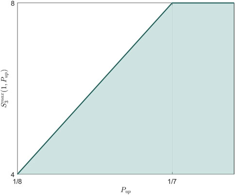
FIGURE 1. The maximal values of Svetlichny inequality $S_3^{\mathit{max}}(G,P_{up})$ that the adversary can fake using the classical system (G = 1) when considering measurement dependence P_up. The shaded region in the figure indicates that no true randomness is generated.

We also illustrate the theorem by presenting it in two cases. As described in Figure 2, for the case of $P_{up}=\frac{1}{8}$ or $P_{\mathit{low}}=\frac{1}{8}$, the inputs are completely random, and the adversary Eve has no a priori knowledge of the inputs. In this case, if Eve constructs a deterministic strategy of outcomes, the Svetlichny inequality cannot be violated. Thus, the adversary Eve cannot fake true randomness. For the case of 7P_up + P_low > 1 or 7P_up + P_low < 1, Eve can obtain part of the information of inputs and then can construct a classical strategy to reach the maximum value of the Svetlichny inequality $S_3^{\mathit{max}}(1,P_{\mathit{low}},P_{up})$. In this case, we conclude that there is true randomness generation when $S_3^{\mathit{obv}}>S_3^{\mathit{max}}(1,P_{\mathit{low}},P_{up})$.

FIGURE 2

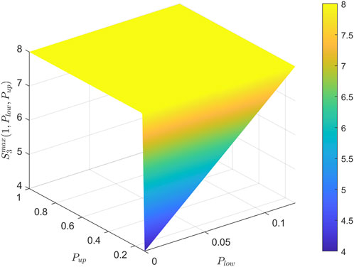
FIGURE 2. The maximal values of Svetlichny inequality $S_3^{\mathit{max}}(G,P_{\mathit{low}},P_{up})$ that the adversary can fake using the classical system (G = 1) when considering measurement dependence P_low and P_up. The color bar corresponds to the upper bound of the Svetlichny inequality. It is easy to know that Figure 1 can be seen as a special case of Figure 2 when P_low = 0.

5 Conclusion

In this paper, we explored the effect of measurement dependence on the tripartite Svetlichny test. Concretely, we showed the relation among measurement dependence, guessing probability, and the maximal violation of Svetlichny inequality that the adversary can fake. Using the degree of measurement dependence with flexible lower and upper bounds, we analyze the case that genuine tripartite nonlocality is nonexistent and give a security analysis of the device-independent quantum information processing tasks. Taking random number generation as an example, we considered the range that the adversary Eve can fake using the classical system. Attempts to the adversary with stronger ability merit further investigation. A natural extension of this work is to explore more different correlations, such as network nonlocality [37] and steering [38].

Data availability statement

The original contributions presented in the study are included in the article/Supplementary Material; further inquiries can be directed to the corresponding authors.

Author contributions

R-ZL: writing–original draft, writing–review and editing, conceptualization, data curation, formal analysis, investigation, methodology, resources, software, supervision, validation, and visualization. D-DL: writing–original draft, writing–review and editing, conceptualization, data curation, formal analysis, and investigation. S-YW: data curation, formal analysis, methodology, project administration, software, visualization, and writing–review and editing. S-JQ: formal analysis, funding acquisition, methodology, project administration, supervision, and writing–review and editing. FG: formal analysis, funding acquisition, writing–original draft, writing–review and editing, and project administration. Q-YW: formal analysis, funding acquisition, project administration, resources, and writing–review and editing.

Funding

The author(s) declare financial support was received for the research, authorship, and/or publication of this article. This work is supported by the National Natural Science Foundation of China (Grant Nos 62272056, 62171056, and 62372048).

Conflict of interest

The authors declare that the research was conducted in the absence of any commercial or financial relationships that could be construed as a potential conflict of interest.

Publisher’s note

All claims expressed in this article are solely those of the authors and do not necessarily represent those of their affiliated organizations, or those of the publisher, the editors, and the reviewers. Any product that may be evaluated in this article, or claim that may be made by its manufacturer, is not guaranteed or endorsed by the publisher.

Supplementary material

The Supplementary Material for this article can be found online at: https://www.frontiersin.org/articles/10.3389/fphy.2024.1356682/full#supplementary-material

References

1. Acín A, Gisin N, Masanes L. From bell’s theorem to secure quantum key distribution. Phys Rev Lett (2006) 97:120405. doi:10.1103/physrevlett.97.120405

PubMed Abstract | CrossRef Full Text | Google Scholar

2. Pironio S, Acín A, Brunner N, Gisin N, Massar S, Scarani V. Device-independent quantum key distribution secure against collective attacks. New J Phys (2009) 11:045021. doi:10.1088/1367-2630/11/4/045021

CrossRef Full Text | Google Scholar

3. Kołodyński J, Máttar A, Skrzypczyk P, Woodhead E, Cavalcanti D, Banaszek K, et al. Device-independent quantum key distribution with single-photon sources. Quantum (2020) 4:260. doi:10.22331/q-2020-04-30-260

CrossRef Full Text | Google Scholar

4. Pironio S, Acín A, Massar S, de La Giroday AB, Matsukevich DN, Maunz P, et al. Random numbers certified by bell’s theorem. Nature (2010) 464:1021–4. doi:10.1038/nature09008

PubMed Abstract | CrossRef Full Text | Google Scholar

5. Acín A, Masanes L. Certified randomness in quantum physics. Nature (2016) 540:213–9. doi:10.1038/nature20119

PubMed Abstract | CrossRef Full Text | Google Scholar

6. Ma X, Yuan X, Cao Z, Qi B, Zhang Z. Quantum random number generation. npj Quan Inf (2016) 2:16021–9. doi:10.1038/npjqi.2016.21

CrossRef Full Text | Google Scholar

7. Liu Y, Zhao Q, Li M-H, Guan J-Y, Zhang Y, Bai B, et al. Device-independent quantum random-number generation. Nature (2018) 562:548–51. doi:10.1038/s41586-018-0559-3

PubMed Abstract | CrossRef Full Text | Google Scholar

8. Mayers D, Yao A. Self testing quantum apparatus (2003). arXiv preprint quant-ph/0307205.

Google Scholar

9. Šupić I, Bowles J. Self-testing of quantum systems: a review. Quantum (2020) 4:337. doi:10.22331/q-2020-09-30-337

CrossRef Full Text | Google Scholar

10. Maitra A, Paul G, Roy S. Device-independent quantum private query. Phys Rev A (2017) 95:042344. doi:10.1103/physreva.95.042344

CrossRef Full Text | Google Scholar

11. Li D, Huang X, Huang W, Gao F, Yan S. Espquery: an enhanced secure scheme for privacy-preserving query based on untrusted devices in the internet of things. IEEE Internet Things J (2020) 8:7229–40. doi:10.1109/jiot.2020.3038928

CrossRef Full Text | Google Scholar

12. Einstein A, Podolsky B, Rosen N. Can quantum-mechanical description of physical reality be considered complete? Phys Rev (1935) 47:777–80. doi:10.1103/physrev.47.777

CrossRef Full Text | Google Scholar

13. Bell JS. On the einstein podolsky rosen paradox. Phys Physique Fizika (1964) 1:195–200. doi:10.1103/physicsphysiquefizika.1.195

CrossRef Full Text | Google Scholar

14. Clauser JF, Horne MA, Shimony A, Holt RA. Proposed experiment to test local hidden-variable theories. Phys Rev Lett (1969) 23:880–4. doi:10.1103/physrevlett.23.880

CrossRef Full Text | Google Scholar

15. Aspect A, Grangier P, Roger G. Experimental realization of einstein-podolsky-rosen-bohm gedankenexperiment: a new violation of bell’s inequalities. Phys Rev Lett (1982) 49:91–4. doi:10.1103/physrevlett.49.91

CrossRef Full Text | Google Scholar

16. Hensen B, Bernien H, Dréau AE, Reiserer A, Kalb N, Blok MS, et al. Loophole-free bell inequality violation using electron spins separated by 1.3 kilometres. Nature (2015) 526:682–6. doi:10.1038/nature15759

PubMed Abstract | CrossRef Full Text | Google Scholar

17. Giustina M, Versteegh MA, Wengerowsky S, Handsteiner J, Hochrainer A, Phelan K, et al. Significant-loophole-free test of bell’s theorem with entangled photons. Phys Rev Lett (2015) 115:250401. doi:10.1103/physrevlett.115.250401

PubMed Abstract | CrossRef Full Text | Google Scholar

18. Shalm LK, Meyer-Scott E, Christensen BG, Bierhorst P, Wayne MA, Stevens MJ, et al. Strong loophole-free test of local realism. Phys Rev Lett (2015) 115:250402. doi:10.1103/physrevlett.115.250402

PubMed Abstract | CrossRef Full Text | Google Scholar

19. Hall MJ. Local deterministic model of singlet state correlations based on relaxing measurement independence. Phys Rev Lett (2010) 105:250404. doi:10.1103/physrevlett.105.250404

PubMed Abstract | CrossRef Full Text | Google Scholar

20. Hall MJ. Relaxed bell inequalities and kochen-specker theorems. Phys Rev A (2011) 84:022102. doi:10.1103/physreva.84.022102

CrossRef Full Text | Google Scholar

21. Koh DE, Hall MJ, Pope JE, Marletto C, Kay A, Scarani V, et al. Effects of reduced measurement independence on bell-based randomness expansion. Phys Rev Lett (2012) 109:160404. doi:10.1103/physrevlett.109.160404

PubMed Abstract | CrossRef Full Text | Google Scholar

22. Pope JE, Kay A. Limited measurement dependence in multiple runs of a bell test. Phys Rev A (2013) 88:032110. doi:10.1103/physreva.88.032110

CrossRef Full Text | Google Scholar

23. Pütz G, Rosset D, Barnea TJ, Liang Y-C, Gisin N. Arbitrarily small amount of measurement independence is sufficient to manifest quantum nonlocality. Phys Rev Lett (2014) 113:190402. doi:10.1103/physrevlett.113.190402

PubMed Abstract | CrossRef Full Text | Google Scholar

24. Pütz G, Gisin N. Measurement dependent locality. New J Phys (2016) 18:055006. doi:10.1088/1367-2630/18/5/055006

CrossRef Full Text | Google Scholar

25. Tan EY-Z, Cai Y, Scarani V. Measurement-dependent locality beyond independent and identically distributed runs. Phys Rev A (2016) 94:032117. doi:10.1103/physreva.94.032117

CrossRef Full Text | Google Scholar

26. Friedman AS, Guth AH, Hall MJ, Kaiser DI, Gallicchio J. Relaxed bell inequalities with arbitrary measurement dependence for each observer. Phys Rev A (2019) 99:012121. doi:10.1103/physreva.99.012121

CrossRef Full Text | Google Scholar

27. Kim M, Lee J, Kim H-J, Kim SW. Tightest conditions for violating the bell inequality when measurement independence is relaxed. Phys Rev A (2019) 100:022128. doi:10.1103/physreva.100.022128

CrossRef Full Text | Google Scholar

28. Hall MJ, Branciard C. Measurement-dependence cost for bell nonlocality: causal versus retrocausal models. Phys Rev A (2020) 102:052228. doi:10.1103/physreva.102.052228

CrossRef Full Text | Google Scholar

29. Šupić I, Bancal J-D, Brunner N. Quantum nonlocality in the presence of strong measurement dependence. Phys Rev A (2023) 108:042207. doi:10.1103/physreva.108.042207

CrossRef Full Text | Google Scholar

30. Kimura G, Susuki Y, Morisue K. Relaxed bell inequality as a trade-off relation between measurement dependence and hiddenness. Phys Rev A (2023) 108:022214. doi:10.1103/physreva.108.022214

CrossRef Full Text | Google Scholar

31. Yuan X, Zhao Q, Ma X. Clauser-horne bell test with imperfect random inputs. Phys Rev A (2015) 92:022107. doi:10.1103/physreva.92.022107

CrossRef Full Text | Google Scholar

32. Yuan X, Cao Z, Ma X. Randomness requirement on the clauser-horne-shimony-holt bell test in the multiple-run scenario. Phys Rev A (2015) 91:032111. doi:10.1103/physreva.91.032111

CrossRef Full Text | Google Scholar

33. Li D-D, Zhou Y-Q, Gao F, Li X-H, Wen Q-Y. Effects of measurement dependence on generalized clauser-horne-shimony-holt bell test in the single-run and multiple-run scenarios. Phys Rev A (2016) 94:012104. doi:10.1103/physreva.94.012104

CrossRef Full Text | Google Scholar

34. Huang X-H, Li D-D, Zhang P. Effects of measurement dependence on tilted chsh bell tests. Quan Inf Process (2018) 17:291–18. doi:10.1007/s11128-018-2060-1

CrossRef Full Text | Google Scholar

35. Li R, Li D, Huang W, Xu B, Gao F. Tight bound on tilted chsh inequality with measurement dependence. Physica A: Stat Mech its Appl (2023) 626:129037. doi:10.1016/j.physa.2023.129037

CrossRef Full Text | Google Scholar

36. Svetlichny G. Distinguishing three-body from two-body nonseparability by a bell-type inequality. Phys Rev D (1987) 35:3066–9. doi:10.1103/physrevd.35.3066

PubMed Abstract | CrossRef Full Text | Google Scholar

37. Šupić I, Bancal J-D, Brunner N. Quantum nonlocality in networks can be demonstrated with an arbitrarily small level of independence between the sources. Phys Rev Lett (2020) 125:240403. doi:10.1103/physrevlett.125.240403

PubMed Abstract | CrossRef Full Text | Google Scholar

38. Uola R, Costa ACS, Nguyen HC, Gühne O. Quantum steering. Rev Mod Phys (2020) 92:015001. doi:10.1103/revmodphys.92.015001

CrossRef Full Text | Google Scholar