Abstract
This study presents a novel method for wideband acoustic analysis using the Boundary Element Method (BEM), addressing significant computational challenges. Traditional BEM requires repetitive computations across different frequencies due to the frequency-dependent system matrix, resulting in high computational costs. To overcome this, the Hankel function is expanded into a Taylor series, enabling the separation of frequency-dependent and frequency-independent components in the boundary integral equations. This results in a frequency-independent system matrix, improving computational efficiency. Additionally, the method addresses the issue of full-rank, asymmetric coefficient matrices in BEM, which complicate the solution of system equations over wide frequency ranges, particularly for large-scale problems. A Reduced-Order Model (ROM) is developed using the Second-Order Arnoldi (SOAR) method, which retains the key characteristics of the original Full-Order Model (FOM). The singularity elimination technique is employed to directly compute the strong singular and super-singular integrals in the acoustic equations. Numerical examples demonstrate the accuracy and efficiency of the proposed approach, showing its potential for large-scale applications in noise control and acoustic design, where fast and precise analysis is crucial.
1 Introduction
In the acoustics domain, simulating and analyzing the propagation of sound waves through complex structures is essential. Frequency sweep calculations play a pivotal role in understanding sound wave behavior across various frequencies, crucial for designing effective acoustic barriers and noise reduction devices. Traditional methods for these calculations often utilize the finite element method (FEM) or the boundary element method (BEM). It is common knowledge that BEM is frequently utilized to address acoustic issues because of its superior accuracy and simplicity in mesh creation [1–4]. For external acoustic problems, it naturally satisfies the Sommerfeld radiation condition at infinity [5–9]. Conventional sound pressure calculations are typically optimized for specific frequencies, limiting their applicability across a broader frequency spectrum. To address this limitation, broadband analysis is introduced to provide results over a wider range of frequencies [10]. Nevertheless, in broadband analysis, the frequency band within a given range is segmented, and the coefficient matrix along with the boundary elements system equation is recalculated at every distinct frequency point. This procedure results in substantial computational expense. This study presents an efficient approach for rapid frequency sweep calculations in broadband acoustics.
When performing broadband acoustic analysis with the BEM, the frequency dependence of the results in coefficient matrices that change with frequency [11, 12]. Consequently, for large-scale issues, the approach is particularly time-consuming because the boundary element system equations must be recalculated for every discrete frequency point. Researchers came up with a number of techniques to speed up the broadband analysis computational process to address this problem [13–16]. A three-dimensional (3D) axisymmetric multifrequency acoustic analysis technique called the Linear Frequency Interpolation Technique (FIT) was proposed by Vanhille et al. [17]. In this approach, the second-order isoparametric segment of the Helmholtz Integral Equation (HIE) is discretized. Despite its effectiveness, FIT requires substantial storage capacity. Li [18] addressed the issue by separating the frequency terms from the damping function through power series expansions of sine and cosine functions into algebraic polynomials, which significantly reduced computational time for multifrequency problems. Similarly, Zhang et al. [19] tackled multifrequency issues using BEM and incorporated series expansion techniques in their calculations, which offer high accuracy and computational efficiency [20]. The advantages of using series expansion are precision and computational economy [21–23]. In this study, the frequency-related and frequency-unrelated components of the product function in the Boundary Integral Equations (BIE) are separated using a Taylor series expansion.
In the realm of acoustic computations using the BEM, coefficient matrices exhibit characteristics of being asymmetric, full-rank, and dense [24, 25]. These attributes contribute to diminished computational efficiency, particularly evident in scenarios involving large-scale problems [26, 27]. Model Order Reduction (MOR) emerges as a viable solution to this challenge [28–31]. Among the most prominent MOR techniques [32] is Proper Orthogonal Decomposition (POD) [33, 34]. However, the quality of the simplified model is not guaranteed, as it depends on the representativeness of the snapshots (or primary frequencies) selected during the POD process [35]. The second-order Arnoldi (SOAR) algorithm for two-dimensional (2D) linear systems, which was introduced by Bai et al. [36, 37], has garnered interest from numerous scholars. The full-order model (FOM) gets mapped onto the projection space. SOAR facilitates the acquisition of an orthogonal basis within the projection space and the construction of a Reduced-Order Model (ROM) that preserves the characteristics of the initial model. Furthermore, the SOAR method finds extensive application in structural acoustic analysis, second-order dynamical system modeling [19], and quadratic eigenvalue problems [37, 38].
Singular Helmholtz boundary integral equations may fail to yield unique solutions when applied to exterior boundary value problems. To address this issue, two primary approaches have been proposed [39–42]. The Combined Helmholtz Integral Equation Formula (CHIEF), cited in Ref. [43], effectively addresses this issue by introducing additional HIE within the internal domain [44, 45]. The resulting overdetermined system of equations can be solved using the method of least squares. However, determining the optimal number and placement of internal points, particularly for issues of high frequency, remains challenging. The Burton-Miller method [46] presents another useful strategy for handling non-unique solutions, offering a linear formulation of the Classical Boundary Integral Equation (CBIE) and its associated Normal Derivative Boundary Integral Equation (NDBIE). If the boundary is nonsmooth, NDBIE becomes hypersingular, requiring special numerical treatment. This study utilizes Cauchy principal value integrals and Hadamard finite part integrals for handling singular integrals.
To enable the application of the Boundary Element Method (BEM) in 2D acoustic computations across a wide frequency range, this study proposes the following enhancements:
Frequency-dependence elimination for the 2D acoustic state boundary integral equation using Taylor series expansion.
A ROM of a 2D acoustic state system based on SOAR is proposed.
The singularity elimination technique is suggested for accurately resolving the singularities in the boundary integrals present in the Taylor series expansion formulation.
This article has the following structure. Section 2 details the BEM formulation for acoustic state analysis. Section 3 elaborates on the BEM formulation with Taylor series expansion for acoustic state analysis. MOR built on the adaptive SOAR method is employed in Section 4 to speed up the BEM computation for 2D broadband acoustic situations. The treatment of singular integrals in kernel function border integrals is described in Section 5. Section 6 includes multiple numerical instances that verify the effectiveness of the proposed algorithm. Finally, conclusions and further discussions are drawn in Section 7.
2 BEM formulations for acoustic state analysis
The Helmholtz half-space problem can be represented by the following BIE and normal derivative boundary integral equation (HBIE).andwhere signifies the field point, denotes the source point, and is the normal derivative of the sound pressure : . When is located on a border that is smooth , . Acoustic pressure incident at position is given by . The function of Green and its derivatives in Equation 1 and Equation 2 are presented as follows, which can be expressed in Equation 3.where the th order first kind Hankel function is indicated by , denotes by the wave number, , is the Cartesian component of or and the distance between the field and source locations is represented by the formula .
For exterior acoustic problems, using either Equation 1 or Equation 2 alone can lead to non-uniqueness of the solution at certain imaginary frequencies. According to the Burton-Miller idea, a linear combination of Equation 1 and Equation 2 can effectively resolve this issue. The Burton-Miller formulation is expressed as follows [46].in which represents the coupling parameter: defined as where and in other cases.
By discretizing the structural boundary into several elements using constant elements and introducing the coefficient matrix, Equation 4 can be reformulated as followswhere and ( indicates the quantity of degrees of freedom.) are the coefficient matrices. They are asymmetric, fully populated, and frequency-related. The column vectors and , respectively, represent the sound pressure and the acoustic flux at the collocation locations. is the vector of the incident wave.
To determine the sound pressure values at the boundary surface nodes, Equation 5 needs to be solved. Subsequently, the sound pressure can be computed at any point within the acoustic domain by using Equation 4 with and .
Its sound pressure, , can be written as follows if the computation takes into account the external acoustic field.where the matrices and as well as the vector are similar to those in Equation 5, except that the source point is outside the structure domain. And and ( indicates the quantity of degrees of freedom.)
3 Frequency sweep analysis for acoustic state
In broadband acoustic analysis using BEM, the frequency-dependent coefficient matrices result in time-consuming repetitive computations and repeated solutions of the system equations, posing challenges for practical engineering applications. This frequency dependence arises because the underlying solution is inherently frequency-related. To address this issue, the frequency dependence of the coefficient matrix is eliminated by applying the Taylor series theorem.
The Taylor series expansion of [47] is given bywhere is a fixed frequency expansion point. As seen in Figure 1, the fixed expansion point in this paper is the midway point of the frequency band.
FIGURE 1
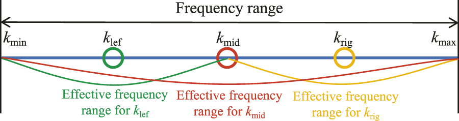
Calculate the frequency band.
Considering an incident wave traveling along the -axis, the Taylor series expansion of the term related to in Equation 4 can be expressed as followswhere denotes the -axis coordinate of the source point, with being either or .
The terms of incident wave in Equation 8 are Taylor series expanded into
The expansion expression for the integral of the kernel functions is obtained by combining Equation 7 and Equation 4.wherewhereBy combining Equation 12 and Equation 9, an expression related to the incident wave in Equation 4 is obtained.where the respective components can be expressed as Equation 14.
A new formulation of Equation 4 is given below by substituting Equation 10 and Equation 13 into Equation 4.By discretizing Equation 15 using constant elements, the following matrix expression is derived.Due to the linearization of the BEM system, the solutions and in Equation 16 with truncation term can be expressed as Equation 17 and Equation 18.andwhere the respective solutions of the following system equations are , , and .
The coefficient matrices , , , and in Equation 19 are frequency unrelated. Thus, it only needs to be solved once for wide-frequency acoustic problems, eliminating the need for repetitive calculations of coefficient matrices in BEM systems. However, there is another disadvantage of this method, which is that it is still very difficult to solve the equations directly using GMRES for large problems with multiple frequencies because the coefficient matrices are full-rank and asymmetric and the truncation terms require high storage capacity . It is evident from observation that Equation 19 is the second-order system equation concerning frequency. An efficient SOAR method is presented in [48] to accelerate the broadband solution of Equation 19.
4 Dimension reduction of BEM system for acoustic state analysis
In this section, an effective SOAR method is proposed to expedite the solution of the coefficient matrix by reducing the dimensionality of the 2D system. This projection technique is predicated on the Krylov subspace of second order. By using the method, a system with an equivalent second-order structure but with a diminished state space dimension is created. In Equation 19, the frequency-independent coefficients , , , and are utilized to construct the frequency-unrelated orthogonal basis iteratively, implementing the SOAR algorithm.
In this work, the scattering of an incident wave by a rigid structural surface is considered. The vectors in Equation 5 vanish because the particle velocity on the surface of the structure is zero. Thus, Equation 19 can be rewritten as
When , the coefficients in Equation 19 are utilized to create frequency-independent orthogonal bases, then Equation 19 is re-expressed as
It should be noted that Equation 21 is not an approximation of the original system equation; rather, it is used for the construction of the orthogonal basis. Equation 21, approximated around a chosen expansion point , can be expressed as Equation 22.where and .
Following the SOAR method procedure outlined in Ref. [48], a sequence of frequency-independent orthogonal bases was constructed in the second-order Krylov subspace using the coefficients from Equation 19, where as shown in Equation 23.where the respective quantities are shown in Equation 24.
To define a reduced system equation of the initial Equation 20, the projection subspace is constructed by spanning a sequence of nonzero columns of . Equation 20 is reformulated as Equation 25.Subsequently, the simplified system equation at the expansion point can be stated as Equation 26.where the coefficient matrix is shown in Equation 27.
The relation between the solution of FOM and ROM is expressed as
is the th order Padé-type approximation of about the fixed expansion point , as shown in Equation 29.
In the ROM, , and are matrices where . This significantly reduced storage requirements and improved computational efficiency. At the collocation points on the structural surface, the sound pressure can be obtained using Equation 28. Afterward, at any point within the acoustic domain, Equation 6 can be used to get the sound pressure value.
5 Singular integral in BEM
The boundary integral of the kernel function in Equation 11 can be expressed as the sum of singular and non-singular terms.where is the element that contains the source point . denotes the boundary that does not contain . Since the integral does not exhibit singularity on the boundary , Gauss quadrature can be employed for its solution. However, the integral over the boundary is singular and must be processed to do a numerical calculation.
The steps for handling singular integrals are as follows:
1. Suppose there is a singular function . First, perform a singular order analysis on the integrand to obtain a simple function that shares the same order of singularity.
2. Then, split the integral of the singular function into two parts: one part is the integrand minus the simple function , and the other part is the integral of the simple function . Since is non-singular, it can be directly computed using Gaussian-Legendre quadrature. Although retains its singularity, its simple form allows for accurate integral results through various methods, such as integration by parts, the Cauchy principal value, and the Hadamard finite part integral.
3. Finally, adding these two parts yields the accurate integral value of the original singular function .
In this study, singular integrals are handled using the Cauchy principal value and the Hadamard finite part integral methods. With reference to Figure 2, let represent a semicircle of radius , and represent . Equation 30 can be used to rewrite the singular integral term in Equation 31.
FIGURE 2

The constant element is connected to an infinitesimal semicircle. Normal derivatives at source points and field points are represented by the notations and , respectively.
When , then , hence , and are all zero. Therefore, the singular integrals in Equation 11 are present only in and .
To facilitate the derivation of singular integrals, the singular terms of and are denoted as and respectively.
Based on Equation 31 and Equation 32, the integrals and in can be restated aswhere and in . The non-singular terms in Equation 33 are computed using Gaussian quadrature. The singular part of is and that of is Thus, their m-th derivatives are represented as Equations 34, 35.and
By substituting Equation 34 into the first equation of Equation 33, the two singular terms and in Equation 33 can be expressed as Equation 36.where is the length of the element.
Similarly, by substituting Equation 34 into the second equation of Equation 33, the expressions for and are obtained.and
By combining Equation 37 and Equation 38, the expression for the singular integral is derived as Equation 39.
6 Numerical example
Three computational examples are presented in this section to evaluate the performance of the proposed algorithm. The research employed the Fortran 90 programming language to conduct numerical simulations. 64 GB of RAM and an Intel (R) Core (TM) i9-10900H Central Processing Unit (CPU) were installed on a desktop computer to perform calculations.
In the simulations, some common parameters are as follows: an incident wave with an amplitude of propagating in the positive -axis direction, expressed as . The medium for the acoustic wave is air, with a density of 1.21 and a speed of 343 .
6.1 Acoustic scattering by an infinitely rigid cylinder
The acoustic scattering from a cylinder can be reduced to a two-dimensional problem by assuming that a plane wave beam acts on an infinitely rigid cylinder (see Figure 3). And a plane wave follows the positive -axis of propagation. The cylinder is centered at (0 , 0 ) with a radius of 1 , and the circumference is discretized using 720 constant boundary elements. Additionally, the coordinates of the calculation point are (3 , 0 ) (see Figure 3).
FIGURE 3
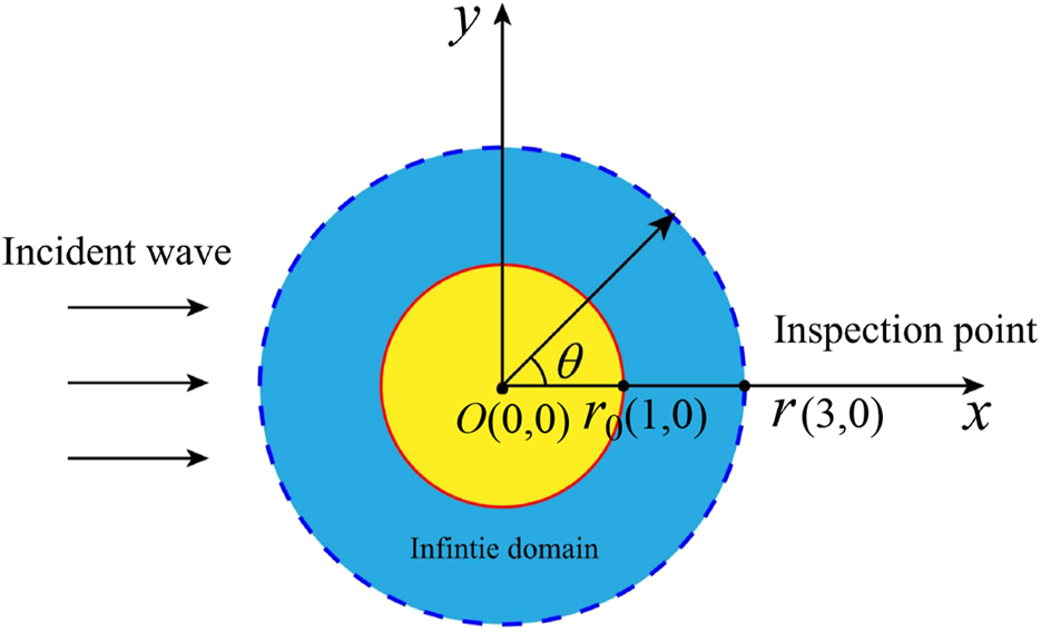
The infinite cylinder serves as the design domain for sound scattering.
The problem of acoustic scattering by an infinitely rigid cylinder has the analytical solution, which is represented as Equation 40 [49].In the above equation, = 1 for = 0, and = 2 otherwise, where represents the Neumann symbols. The expansion consists of 50 terms, and at the detection point, = 0.
The relative error between the numerical result computed and the analytical solution is evaluated, as shown in Equation 41, to ensure that the proposed approach is accurate.where denotes the computational points within the domain, the numerical solution for sound pressure is represented by , and the analytical solution for sound pressure is denoted by . The number of computed points, = 720, is evenly distributed along the perimeter of the circle shown in Figure 3, which has a radius of 3 .
Figure 4 shows the sound pressure amplitude at the computed location (3 , 0 ) obtained using the proposed algorithm. The analytical solution and this outcome are contrasted. Numerical simulations considered two distinct intervals (300, 400) Hz and (400, 500) Hz. In the frequency interval , the fixed expansion point is the midpoint frequency 2. “”, “”, and “” denote the retention of the first 3, 6, and 8 terms of the Taylor expansion, respectively. The ROM attainments by the SOAR approach have an order of 10.
FIGURE 4
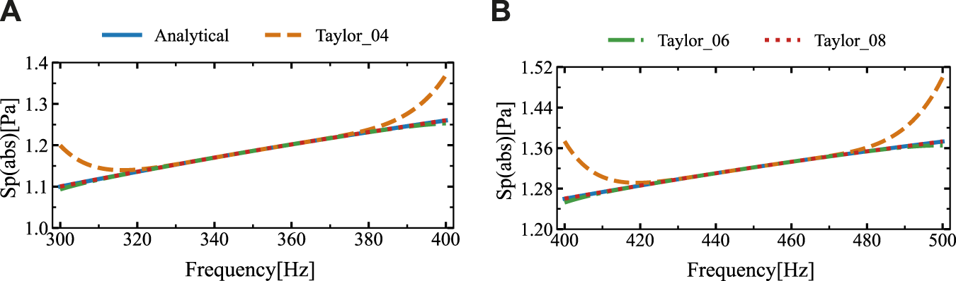
The sound pressure amplitudes at the computational point located at (3 m, 0 m) in two different frequency ranges were obtained using the analytical solution and SOAR Accelerated Taylor Extension-based BEM: (A). f = (300,400) Hz, (B). f = (400,500) Hz.
Figure 4 demonstrates that the sound pressure amplitude values derived from various Taylor series terms of the proposed algorithm are comparatively consistent with the analytical solution. Due to the fixed expansion point being the midpoint of the frequency interval, significant differences occur at the two ends of each frequency interval. In order to minimize the disparity between the analytical and numerical solutions, we subdivided the frequency intervals (300, 400) Hz and (400, 500) Hz into four sub-intervals each, and then recalculated the numerical simulations.
Figure 5 presents the results of the analytical and numerical solutions for the four sub-intervals after subdivision. It is evident that the numerical solutions match the analytical solutions very closely. Figure 6 shows the relative errors between them. Based on the observations, it can be inferred that the relative error is sufficiently minimal and exhibits little fluctuation when six or more expansion terms are used.
FIGURE 5
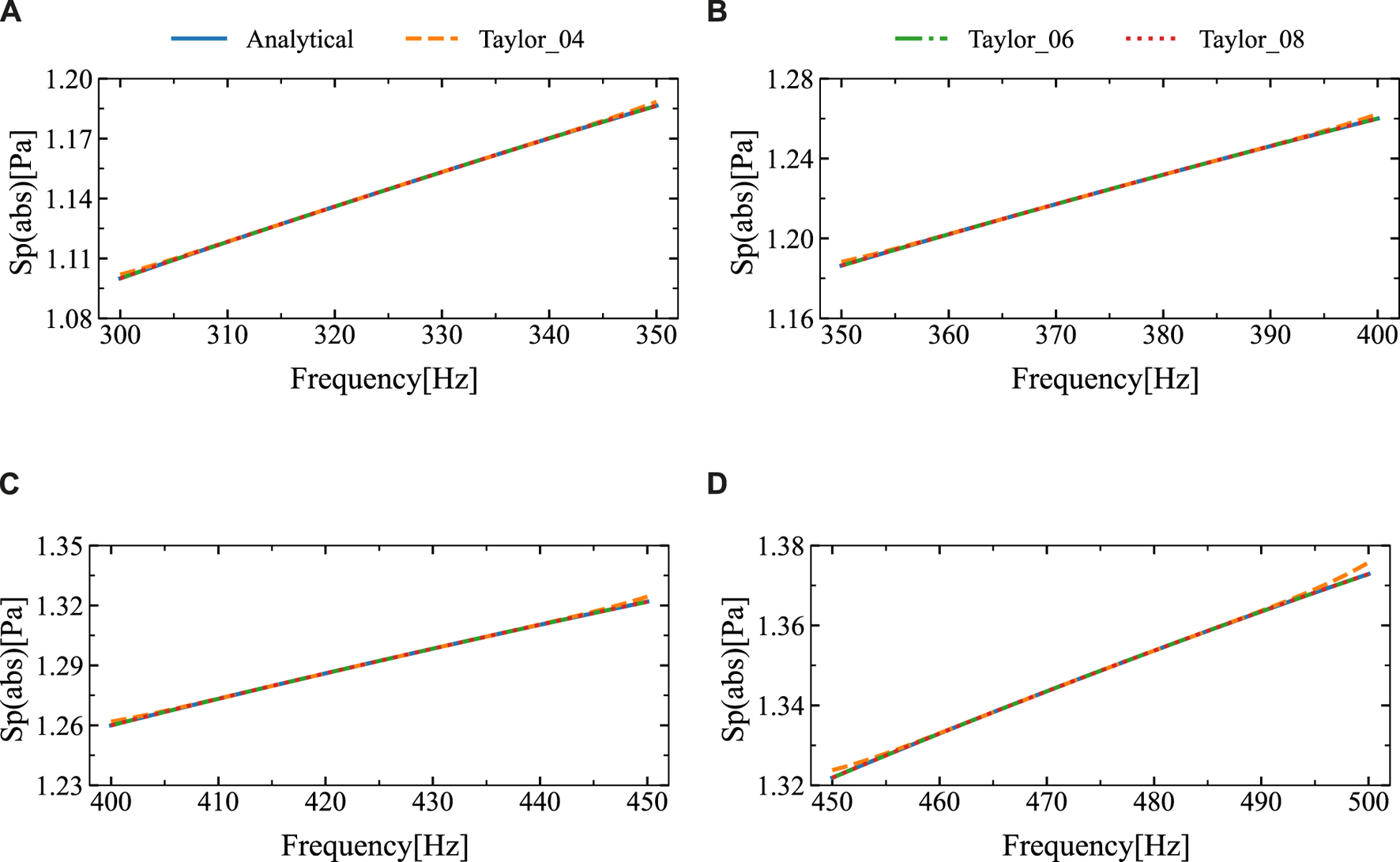
The sound pressure amplitudes at the computational point located at (3 m, 0 m) in four different frequency ranges were obtained using the analytical solution and SOAR Accelerated Taylor Extension-based BEM: (A). f = (300,350) Hz, (B). f = (350,400) Hz, (C). f = (400,450) Hz, (D). f = (450,500) Hz.
FIGURE 6
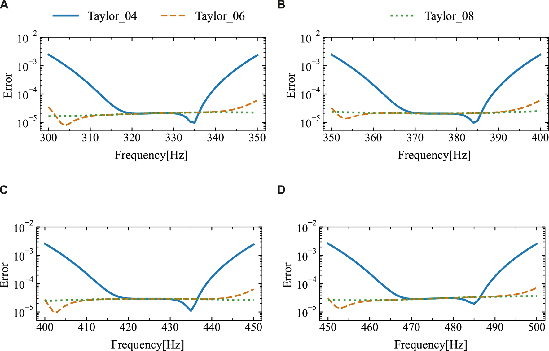
The relative error of the sound pressure at the point of calculation (3 m, 0 m) for different expansion terms was derived through the utilization of the analytical solution and SOAR Accelerated Taylor Extension-based BEM: (A). f = (300,350) Hz, (B). f = (350,400) Hz, (C). f = (400,450) Hz, (D). f = (450,500) Hz.
Figure 7 illustrates how long it takes to compute the point sound pressure amplitude using both the conventional boundary element method (DBEM) and the proposed approach. The frequency sweep range is (300, 400) Hz, with the number of frequency sweeps set to 200 and 1,000, respectively. The ROM attainments by the SOAR approach have an order of 10. It can be observed that for wide-frequency sweep calculations, when compared to the DBEM, the proposed method takes a lot shorter amounts of time. Moreover, the more frequency sweeps performed, the greater the time savings, indicating higher efficiency. Based on the above analysis, six terms for the Taylor series expansion are advised in computational simulations to minimize CPU time.
FIGURE 7
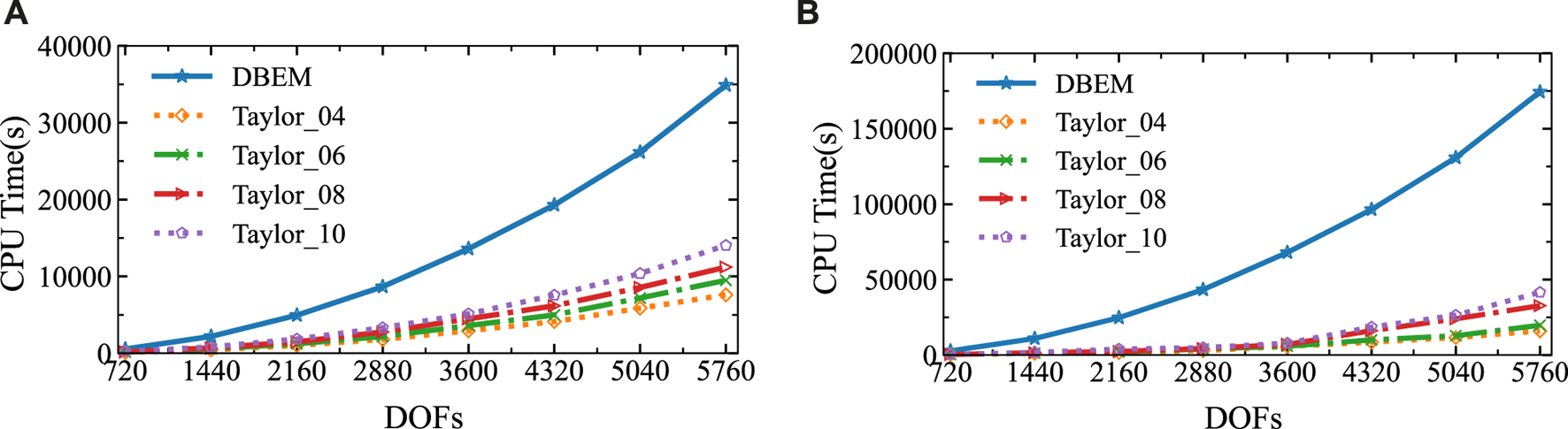
The sound pressure amplitudes at the computational point located at (3 m, 0 m) in two different frequency ranges were obtained using the analytical solution and SOAR Accelerated Taylor Extension-based BEM: (A). Frequency step length = 0.5 Hz., (B). Frequency step length = 0.1 Hz.
6.2 Acoustic scattering by tree-shaped sound barriers
Traffic noise is a major source of environmental noise in urban areas, significantly impacting health and quality of life. The use of sound barriers can mitigate the effects of traffic noise on both the environment and human health.
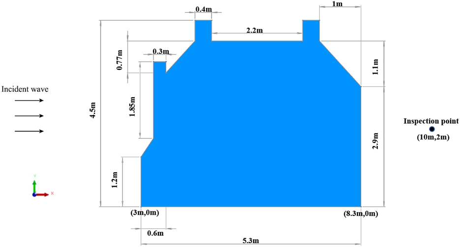
Figure 8 depicts a tree-shaped sound barrier model, where the model boundary is discretized into 868 scattered points by constant elements. The remaining parameters for the tree-shaped sound barrier model are as follows: the trunk and four branches of the tree-shaped sound barrier are each 0.5 in length and 0.3 in width. The base of the trunk measures 0.8 in length and 0.3 in width. A Tree-shaped sound barrier scatters a plane wave that is traveling along the positive -axis with an amplitude of 1. The observation point is located at (14 , 2 ).
FIGURE 8
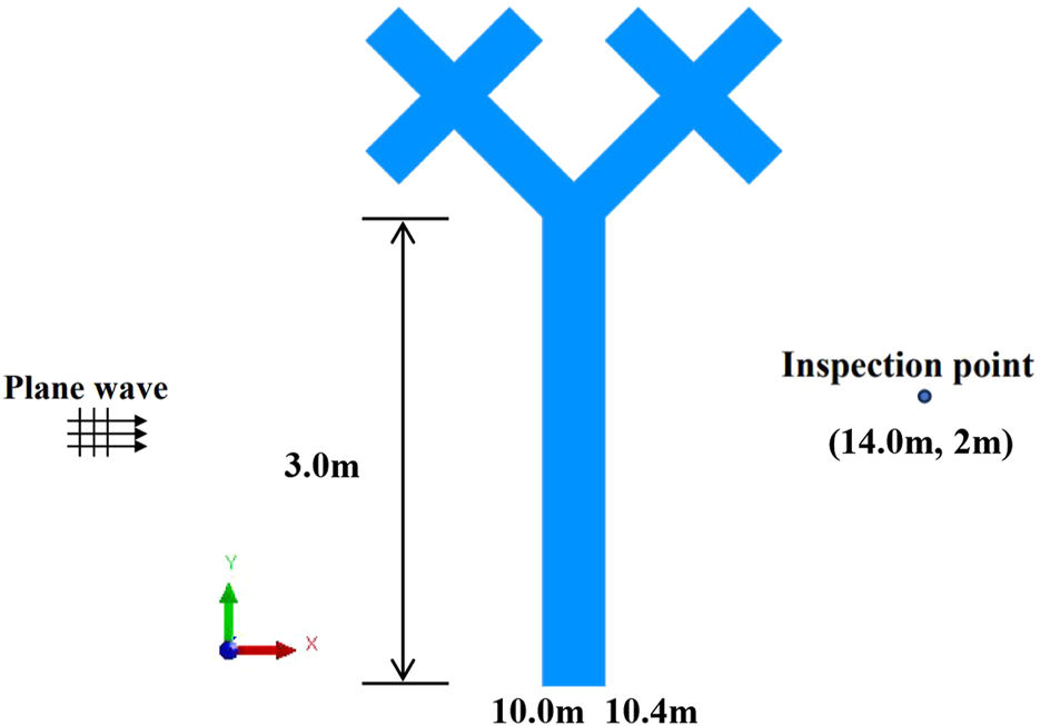
The design domain of the tree-shaped sound barrier model.
Figure 9 depicts the amplitude, imaginary part and real part of the sound pressure at the observation point, obtained using the traditional boundary element method and different Taylor series expansion terms of the proposed algorithm. The figure shows that as the number of Taylor expansion terms increases, the sound pressure results obtained by the proposed approach converge. Due to the fixed frequency expansion point being located at the midpoint of the frequency range, discrepancies appear at the ends of the interval, whereas other regions show good agreement. The frequency band of (150, 200) Hz is split into two sub-intervals, and numerical simulations are conducted separately for each sub-interval. The simulation results are shown in Figure 10. From Figure 10, it can be concluded that the results obtained with different Taylor expansion terms are in high agreement with those obtained using the DBEM.
FIGURE 9
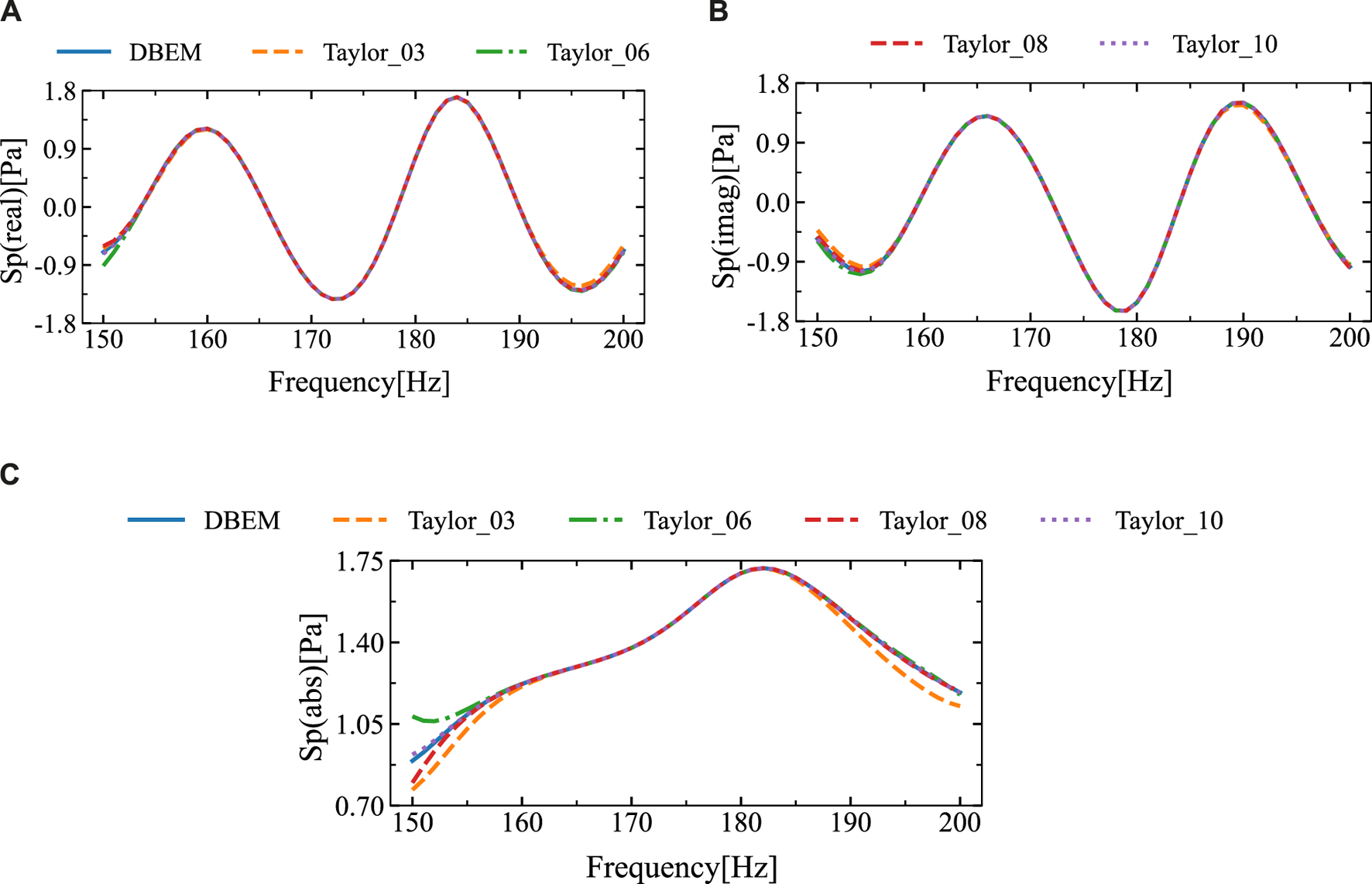
The sound pressure findings at a computing position (14 m, 2 m) that were acquired using DBEM and SOAR Accelerated Taylor Extension-based BEM: (A). Real part, (B). Imaginary part, (C). Sound pressure amplitude.
FIGURE 10
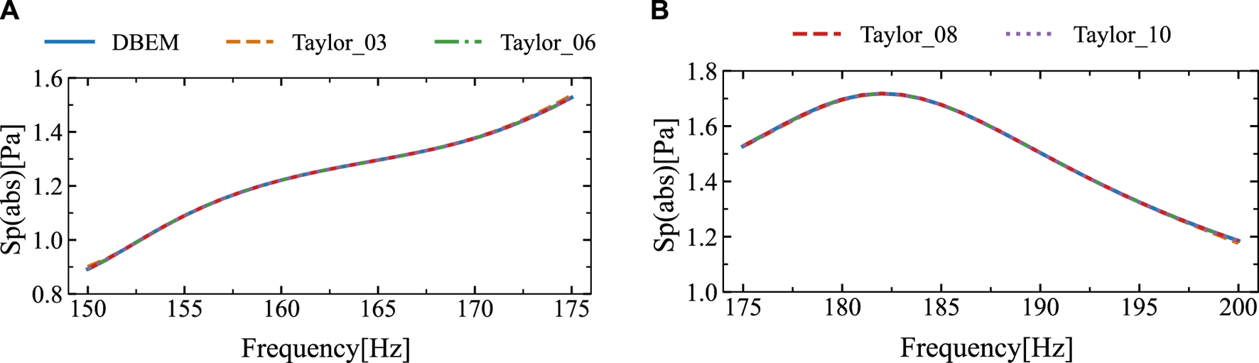
At a point of computation (14 m, 2 m), the sound pressure amplitude were acquired using DBEM and SOAR Accelerated Taylor Extension-based BEM: (A). f = (150,175) Hz, (B). f = (175,200) Hz.
Figure 11 presents the relative error between the results at the calculation points for different expansion terms and those from the traditional boundary element method. The figure indicates that if there are six or more Taylor expansion terms, the relative error remains consistently low and stable. Table 1 displays the sound pressure amplitudes at various frequency points obtained through two different algorithms, along with the relative errors between them.
FIGURE 11
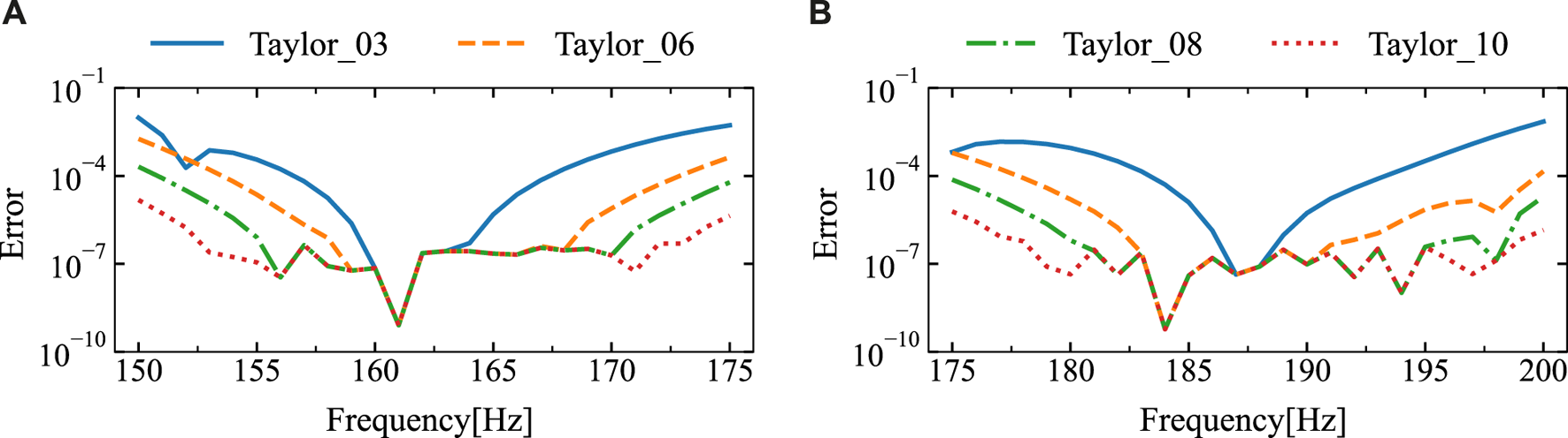
The relative error of the sound pressure at the point of calculation (14 m, 2 m) for different expansion terms was derived through the utilization of the DBEM and SOAR Accelerated Taylor Extension-based BEM: (A). f = (150,175) Hz, (B). f = (175,200) Hz.
TABLE 1
| Frequency | DBEM | Taylor_03 | Taylor_06 | Taylor_08 | Taylor_10 | ||||
|---|---|---|---|---|---|---|---|---|---|
| 150 | 0.89217 | 0.90074 | 9 | 0.89053 | 1 | 0.89235 | 2 | 0.89215 | 2 |
| 155 | 1.08997 | 1.08959 | 3 | 1.08995 | 2 | 1.08998 | 9 | 1.08998 | 9 |
| 160 | 1.22135 | 1.22131 | 3 | 1.22132 | 3 | 1.22137 | 2 | 1.22136 | 8 |
| 165 | 1.29554 | 1.29557 | 2 | 1.29556 | 2 | 1.29555 | 9 | 1.29555 | 8 |
| 170 | 1.37634 | 1.37727 | 7 | 1.37632 | 1 | 1.37633 | 7 | 1.37633 | 7 |
| 175 | 1.52724 | 1.53539 | 5 | 1.52657 | 4 | 1.52733 | 6 | 1.52723 | 7 |
| 180 | 1.69679 | 1.69526 | 9 | 1.69681 | 1 | 1.69678 | 6 | 1.69678 | 6 |
| 185 | 1.67760 | 1.67758 | 1 | 1.67759 | 6 | 1.67759 | 6 | 1.67759 | 6 |
| 190 | 1.50347 | 1.50345 | 1 | 1.50346 | 7 | 1.50346 | 7 | 1.50346 | 7 |
| 195 | 1.32502 | 1.32549 | 4 | 1.32500 | 2 | 1.32501 | 8 | 1.32501 | 8 |
| 200 | 1.18539 | 1.17692 | 7 | 1.18556 | 1 | 1.18536 | 3 | 1.18538 | 8 |
Sound pressure values and relative errors for different taylor expansion terms.
6.3 Acoustic scattering by room
This section demonstrates the calculation of sound pressure amplitudes at observation points within a two-dimensional room. Both the BEM and the Taylor series expansion-based BEM accelerated by the SOAR algorithm are employed. The results from these methods are then compared and analyzed. As depicted in Figure 12, the two-dimensional room model measures 4.5 in height and 5.3 in width. The boundary is divided into 994 discrete points using constant elements. A wave with an amplitude of 1, traveling in the positive -direction, is scattered by the room. The observation point is situated at (10 ,2 ).
FIGURE 12
Acoustic scattering design domain for two-dimensional room.
The frequency range scanned in Figure 13 spans from 200 Hz to 250 Hz and from 250 Hz to 300 Hz. Figure 13 indicates that the sound pressure amplitudes obtained by both methods exhibit good agreement within the intervals of (210, 235) Hz and (260, 290) Hz, but show significant discrepancies at the ends of these intervals. The discrepancy arises because the frequencies used for calculations within each frequency sweep interval are centered on the midpoint of the interval. Consequently, the further a frequency is from the midpoint, the greater the error in the calculated result. To enhance accuracy and diminish errors, the intervals (200, 250) Hz and (250, 300) Hz are subdivided into four sub-intervals each. Within each sub-interval, calculations are performed using the midpoint frequency. The outcomes are illustrated in Figure 14. Figure 14 indicates a high level of agreement between the results obtained by the two algorithms, this suggests that narrowing the intervals to enhance the precision of the algorithm proposed is effective.
FIGURE 13
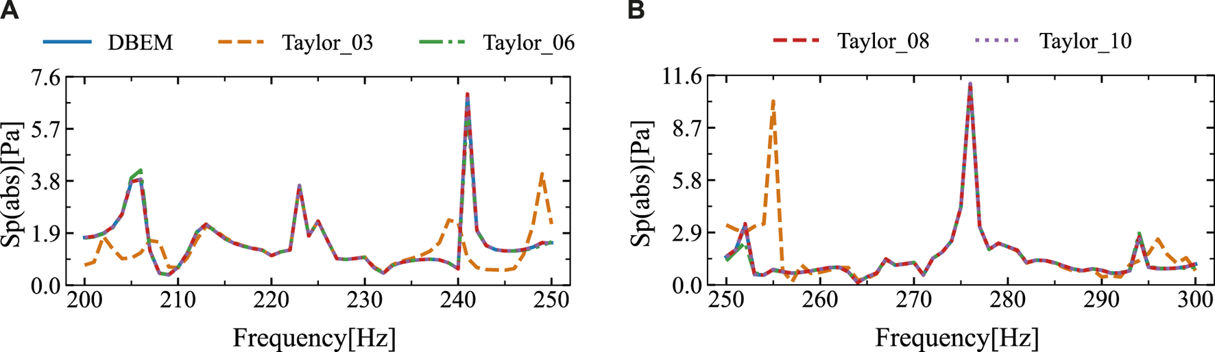
The sound pressure amplitudes at the computational point located at (10 m, 2 m) in four different frequency ranges were obtained using the DBEM and SOAR Accelerated Taylor Extension-based BEM: (A). f = (200,250) Hz, (B). f = (250,300) Hz.
FIGURE 14
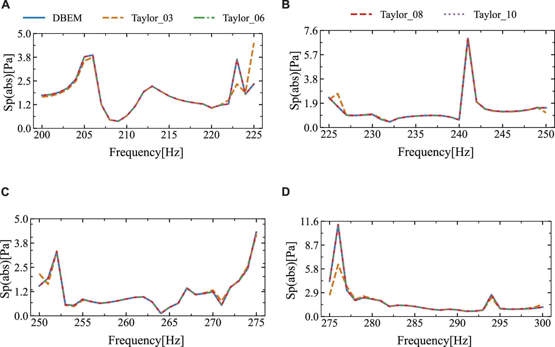
The sound pressure amplitudes at the computational point located at (10 m, 2 m) in four different frequency ranges were obtained using the DBEM and SOAR Accelerated Taylor Extension-based BEM: (A). f = (200,225) Hz, (B). f = (225,250) Hz, (C). f = (250,275) Hz, (D). f = (275,300) Hz.
Figure 15 illustrates the errors between the two algorithms. It is evident that with six or more terms in the Taylor series expansion, the error remains stable and within an acceptable range. Table 2 presents the sound pressure amplitudes and corresponding relative errors at different frequency points.
FIGURE 15
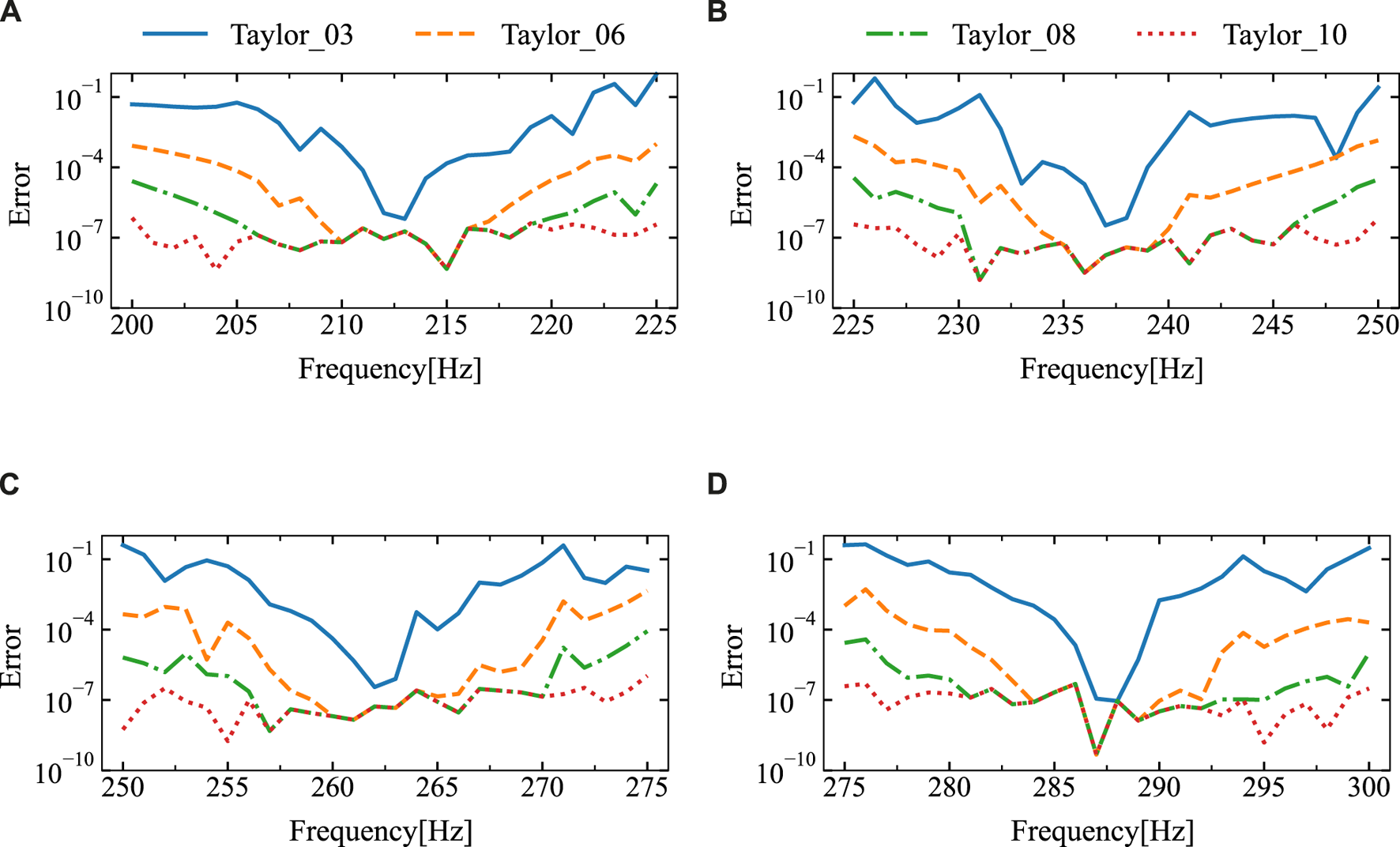
The relative error of the sound pressure at the point of calculation (10 m, 2 m) for different expansion terms was derived through the utilization of the DBEM and SOAR Accelerated Taylor Extension-based BEM: (A). f = (200,225) Hz, (B). f = (225,250) Hz, (C). f = (250,275) Hz, (D). f = (275,300) Hz.
TABLE 2
| Frequency | DBEM | Taylor_03 | Taylor_06 | Taylor_08 | Taylor_10 | ||||
|---|---|---|---|---|---|---|---|---|---|
| 200 | 1.73971 | 1.65520 | 5 | 1.73826 | 8 | 1.73975 | 3 | 1.73971 | 7 |
| 205 | 3.77269 | 3.55690 | 6 | 3.77243 | 7 | 3.77270 | 5 | 3.77269 | 7 |
| 210 | 0.65607 | 0.65559 | 7 | 0.65607 | 6 | 0.65607 | 6 | 0.65607 | 6 |
| 215 | 1.69961 | 1.69936 | 1 | 1.69961 | 5 | 1.69961 | 5 | 1.69961 | 5 |
| 220 | 1.08095 | 1.06445 | 2 | 1.08098 | 3 | 1.08095 | 7 | 1.08095 | 2 |
| 225 | 2.33577 | 2.19804 | 6 | 2.33345 | 1 | 2.33582 | 2 | 2.33577 | 4 |
| 230 | 1.01752 | 1.05120 | 3 | 1.01745 | 7 | 1.01753 | 1 | 1.01753 | 1 |
| 235 | 0.89543 | 0.89551 | 9 | 0.89543 | 5 | 0.89543 | 6 | 0.89543 | 6 |
| 240 | 0.59929 | 0.60016 | 1 | 0.59929 | 2 | 0.59929 | 1 | 0.59929 | 1 |
| 245 | 1.25059 | 1.23222 | 1 | 1.25055 | 4 | 1.25059 | 5 | 1.25059 | 5 |
| 250 | 1.54559 | 1.15591 | 2 | 1.54341 | 1 | 1.54564 | 3 | 1.54559 | 7 |
| 255 | 0.85390 | 0.81109 | 5 | 0.85373 | 2 | 0.85390 | 1 | 0.85390 | 2 |
| 260 | 0.86751 | 0.86747 | 4 | 0.86751 | 2 | 0.86751 | 2 | 0.86751 | 2 |
| 265 | 0.44207 | 0.44203 | 1 | 0.44207 | 1 | 0.44207 | 8 | 0.44207 | 8 |
| 270 | 1.23592 | 1.32387 | 7 | 1.23587 | 4 | 1.23592 | 1 | 1.23592 | 8 |
| 275 | 4.30881 | 4.16733 | 3 | 4.32828 | 5 | 4.30844 | 9 | 4.30882 | 1 |
| 280 | 2.11202 | 2.16971 | 3 | 2.11221 | 9 | 2.11202 | 8 | 2.11202 | 2 |
| 285 | 1.22514 | 1.22547 | 3 | 1.22514 | 2 | 1.22514 | 2 | 1.22514 | 2 |
| 290 | 0.80695 | 0.80552 | 2 | 0.80695 | 9 | 0.80695 | 3 | 0.80695 | 3 |
| 295 | 0.97933 | 0.94893 | 3 | 0.97935 | 2 | 0.97933 | 1 | 0.97933 | 2 |
| 300 | 1.14332 | 1.48699 | 3 | 1.14355 | 2 | 1.14333 | 1 | 1.14332 | 3 |
Sound pressure values and relative errors for different taylor expansion terms.
By comparing the three cases, it is evident that the frequency sweep range is significantly reduced in more complex models. This indicates that the complexity of the model affects the accuracy of the proposed algorithm. However, precise calculations can still be achieved by narrowing the frequency sweep range.
7 Conclusion
This paper employs the BEM to compute sound pressure for frequency scanning analysis. It introduces an efficient computational approach, which includes:
1. The Taylor expansion method decomposes the integral of boundary elements into frequency-related and frequency-unrelated terms, thus eliminating the frequency dependence in the coefficient matrix.
2. By reducing the order of the original system model through the application of the SOAR method, the computational performance for solving large-scale problems was improved.
The algorithm proposed in this paper has potential applications in various engineering fields. For example, in the design of sound barriers, it can be used to quickly assess the acoustic performance of different design options, thereby optimizing the design process. In noise control engineering, this method can be employed to simulate and analyze noise propagation in complex environments, enhancing the effectiveness of noise control measures. We believe that these applications highlight the practical significance of our research and its potential to contribute to real-world engineering challenges. Future work will involve applying the proposed algorithm to problems involving broadband sensitivity scanning and topology optimization.
Statements
Data availability statement
The original contributions presented in the study are included in the article/supplementary material, further inquiries can be directed to the corresponding authors.
Author contributions
SZ: Conceptualization, Software, Writing–original draft. XJ: Methodology, Software, Writing–review and editing. JD: Conceptualization, Data curation, Writing–review and editing. JL: Data curation, Methodology, Software, Writing–review and editing.
Funding
The author(s) declare that no financial support was received for the research, authorship, and/or publication of this article.
Conflict of interest
The authors declare that the research was conducted in the absence of any commercial or financial relationships that could be construed as a potential conflict of interest.
Publisher’s note
All claims expressed in this article are solely those of the authors and do not necessarily represent those of their affiliated organizations, or those of the publisher, the editors and the reviewers. Any product that may be evaluated in this article, or claim that may be made by its manufacturer, is not guaranteed or endorsed by the publisher.
References
1.
Marburg S . Six boundary elements per wavelength: is that enough?J Comput Acoust (2002) 10:25–51. 10.1142/s0218396x02001401
2.
Marburg S Schneider S . Influence of element types on numeric error for acoustic boundary elements. J Comput Acoust (2003) 11:363–86. 10.1142/s0218396x03001985
3.
Qu Y Zhou Z Chen L Lian H Li X Hu Z et al Uncertainty quantification of vibro-acoustic coupling problems for robotic manta ray models based on deep learning. Ocean Eng (2024) 299:117388. 10.1016/j.oceaneng.2024.117388
4.
Chen L Lian H Liu Z Gong Y Zheng C Bordas S . Bi-material topology optimization for fully coupled structural-acoustic systems with isogeometric fem–bem. Eng Anal Boundary Elem (2022) 135:182–95. 10.1016/j.enganabound.2021.11.005
5.
Chen L Lian H Liu Z Chen H Atroshchenko E Bordas SPA . Structural shape optimization of three dimensional acoustic problems with isogeometric boundary element methods. Comput Methods Appl Mech Eng (2019) 355:926–51. 10.1016/j.cma.2019.06.012
6.
Sommerfeld A . Partial differential equations in physics. Academic Press (1949).
7.
Chen L Huo R Lian H Yu B Zhang M Natarajan S et al Uncertainty quantification of 3d acoustic shape sensitivities with generalized nth-order perturbation boundary element methods. Comput Methods Appl Mech Eng (2025) 433:117464. 10.1016/j.cma.2024.117464
8.
Preuss S Gurbuz C Jelich C Baydoun SK Marburg S . Recent advances in acoustic boundary element methods. J Theor Comput Acoust (2022) 30:2240002. 10.1142/s2591728522400023
9.
Chen L Lian H Pei Q Meng Z Jiang S Dong H-W et al Fem-bem analysis of acoustic interaction with submerged thin-shell structures under seabed reflection conditions. Ocean Eng (2024) 309:118554. 10.1016/j.oceaneng.2024.118554
10.
Sobolev A . Wide-band sound-absorbing structures for aircraft engine ducts. Acoust Phys (2000) 46:466–73. 10.1134/1.29911
11.
Wang Z Zhao Z Liu Z Huang Q . A method for multi-frequency calculation of boundary integral equation in acoustics based on series expansion. Appl Acoust (2009) 70:459–68. 10.1016/j.apacoust.2008.05.005
12.
Chen L Zhao J Lian H Yu B Atroshchenko E Li P . A bem broadband topology optimization strategy based on taylor expansion and soar method—application to 2d acoustic scattering problems. Int J Numer Methods Eng (2023) 124:5151–82. 10.1002/nme.7345
13.
Wu T Li W Seybert A . An efficient boundary element algorithm for multi-frequency acoustical analysis. The J Acoust Soc America (1993) 94:447–52. 10.1121/1.407056
14.
Kirkup SM Henwood DJ . Methods for speeding up the boundary element solution of acoustic radiation problems. J Vibration Acoust (1992) 114:374–80. 10.1115/1.2930272
15.
Marburg S Schneider S . Performance of iterative solvers for acoustic problems. part i. solvers and effect of diagonal preconditioning. Eng Anal Boundary Elem (2003) 27:727–50. 10.1016/s0955-7997(03)00025-0
16.
Gao Z Li Z Liu Y . A time-domain boundary element method using a kernel-function library for 3d acoustic problems. Eng Anal Boundary Elem (2024) 161:103–12. 10.1016/j.enganabound.2024.01.001
17.
Vanhille C Lavie A . An efficient tool for multi-frequency analysis in acoustic scattering or radiation by boundary element method. Acta Acustica United Acustica (1998) 84:884–93.
18.
Li S . An efficient technique for multi-frequency acoustic analysis by boundary element method. J Sound Vibration (2005) 283:971–80. 10.1016/j.jsv.2004.05.027
19.
Zhang Q Mao Y Qi D Gu Y . An improved series expansion method to accelerate the multi-frequency acoustic radiation prediction. J Comput Acoust (2015) 23:1450015. 10.1142/s0218396x14500155
20.
Poungthong P Giacomin A Kolitawong C . Series expansion for normal stress differences in large-amplitude oscillatory shear flow from oldroyd 8-constant framework. Phys Fluids (2020) 32:023107. 10.1063/1.5143566
21.
Chen L Lian H Xu Y Li S Liu Z Atroshchenko E et al Generalized isogeometric boundary element method for uncertainty analysis of time-harmonic wave propagation in infinite domains. Appl Math Model (2023) 114:360–78. 10.1016/j.apm.2022.09.030
22.
Cao G Yu B Chen L Yao W . Isogeometric dual reciprocity bem for solving non-fourier transient heat transfer problems in fgms with uncertainty analysis. Int J Heat Mass Transfer (2023) 203:123783. 10.1016/j.ijheatmasstransfer.2022.123783
23.
Liu Z Bian P-L Qu Y Huang W Chen L Chen J A galerkin approach for analysing coupling effects in the piezoelectric semiconducting beams. Eur J Mechanics-A/Solids (2024) 103:105145. 10.1016/j.euromechsol.2023.105145
24.
Li R Liu Y Ye W . A fast direct boundary element method for 3d acoustic problems based on hierarchical matrices. Eng Anal Boundary Elem (2023) 147:171–80. 10.1016/j.enganabound.2022.11.035
25.
Chen L Liu L Zhao W Liu C . An isogeometric approach of two dimensional acoustic design sensitivity analysis and topology optimization analysis for absorbing material distribution. Comput Methods Appl Mech Eng (2018) 336:507–32. 10.1016/j.cma.2018.03.025
26.
Li Q Sigmund O Jensen JS Aage N . Reduced-order methods for dynamic problems in topology optimization: a comparative study. Comput Methods Appl Mech Eng (2021) 387:114149. 10.1016/j.cma.2021.114149
27.
Chen L Lu C Lian H Liu Z Zhao W Li S et al Acoustic topology optimization of sound absorbing materials directly from subdivision surfaces with isogeometric boundary element methods. Comput Methods Appl Mech Eng (2020) 362:112806. 10.1016/j.cma.2019.112806
28.
Chen L Wang Z Lian H Ma Y Meng Z Li P et al Reduced order isogeometric boundary element methods for cad-integrated shape optimization in electromagnetic scattering. Comput Methods Appl Mech Eng (2024) 419:116654. 10.1016/j.cma.2023.116654
29.
Chen L Lian H Dong H-W Yu P Jiang S Bordas SPA . Broadband topology optimization of three-dimensional structural-acoustic interaction with reduced order isogeometric fem/bem. J Comput Phys (2024) 509:113051. 10.1016/j.jcp.2024.113051
30.
Bai Z . Krylov subspace techniques for reduced-order modeling of large-scale dynamical systems. Appl Numer Math (2002) 43:9–44. 10.1016/s0168-9274(02)00116-2
31.
Shen X Du C Jiang S Zhang P Chen L . Multivariate uncertainty analysis of fracture problems through model order reduction accelerated sbfem. Appl Math Model (2024) 125:218–40. 10.1016/j.apm.2023.08.040
32.
Chatterjee A . An introduction to the proper orthogonal decomposition. Curr Sci (2000) 808–17.
33.
Pearson K . One lines and planes of closest fit to systems of points in space. Philosophical Mag (1901) 2:559–72. 10.1080/14786440109462720
34.
Chen L Cheng R Li S Lian H Zheng C Bordas SPA . A sample-efficient deep learning method for multivariate uncertainty qualification of acoustic–vibration interaction problems. Comput Methods Appl Mech Eng (2022) 393:114784. 10.1016/j.cma.2022.114784
35.
Chinesta F Ladevèze P . Separated representations and pgd-based model reduction. Int Centre Mech Siences, Courses Lectures (2014) 554:24.
36.
Bai Z-j. Su Y-f. Second-order krylov subspace and arnoldi procedure, 8. Springer: Journal of Shanghai University (English Edition (2004) p. 378–90. 10.1007/s11741-004-0048-9
37.
Bai Z Su Y . Soar: a second-order arnoldi method for the solution of the quadratic eigenvalue problem. SIAM J Matrix Anal Appl (2005) 26:640–59. 10.1137/s0895479803438523
38.
Yang C . Solving large-scale eigenvalue problems in scidac applications. J Phys Conf Ser (2005) 16:425–34. 10.1088/1742-6596/16/1/058
39.
Zhang Y Gong Y Gao X . Calculation of 2d nearly singular integrals over high-order geometry elements using the sinh transformation. Eng Anal Boundary Elem (2015) 60:144–53. 10.1016/j.enganabound.2014.12.006
40.
Marburg S . The burton and miller method: unlocking another mystery of its coupling parameter. J Comput Acoust (2016) 24:1550016. 10.1142/s0218396x15500162
41.
Gong Y Trevelyan J Hattori G Dong C . Hybrid nearly singular integration for isogeometric boundary element analysis of coatings and other thin 2d structures. Comput Methods Appl Mech Eng (2019) 346:642–73. 10.1016/j.cma.2018.12.019
42.
Liu H Wang F Qiu L Chi C . Acoustic simulation using singular boundary method based on loop subdivision surfaces: a seamless integration of cad and cae. Eng Anal Boundary Elem (2024) 158:97–106. 10.1016/j.enganabound.2023.10.022
43.
Schenck HA . Improved integral formulation for acoustic radiation problems. The J Acoust Soc America (1968) 44:41–58. 10.1121/1.1911085
44.
Chen J-T Chen I Chen K . Treatment of rank deficiency in acoustics using svd. J Comput Acoust (2006) 14:157–83. 10.1142/s0218396x06002998
45.
Chen L Lian H Natarajan S Zhao W Chen X Bordas S . Multi-frequency acoustic topology optimization of sound-absorption materials with isogeometric boundary element methods accelerated by frequency-decoupling and model order reduction techniques. Comput Methods Appl Mech Eng (2022) 395:114997. 10.1016/j.cma.2022.114997
46.
Burton A Miller G . The application of integral equation methods to the numerical solution of some exterior boundary-value problems. Proc R Soc Lond A. Math Phys Sci (1971) 323:201–10. 10.1098/rspa.1971.0097
47.
Zhou H Liu Y Wang J . Optimizing orthogonal-octahedron finite-difference scheme for 3d acoustic wave modeling by combination of taylor-series expansion and remez exchange method. Exploration Geophys (2021) 52:335–55. 10.1080/08123985.2020.1826890
48.
Bai Z Su Y . Dimension reduction of large-scale second-order dynamical systems via a second-order arnoldi method. SIAM J Scientific Comput (2005) 26:1692–709. 10.1137/040605552
49.
Junger MC Feit D Sound, structures, and their interaction, 225. Cambridge, MA: MIT press (1986).
Summary
Keywords
boundary element method, SOAR, Taylor expansion, sound barrier, acoustic scattering
Citation
Zhong S, Jiang X, Du J and Liu J (2024) A reduced-order boundary element method for two-dimensional acoustic scattering. Front. Phys. 12:1464716. doi: 10.3389/fphy.2024.1464716
Received
15 July 2024
Accepted
18 November 2024
Published
05 December 2024
Volume
12 - 2024
Edited by
Leilei Chen, Huanghuai University, China
Reviewed by
Xudong Li, Chinese Academy of Sciences (CAS), China
Jing Fang, Dalian Maritime University, China
Lu Meng, Taiyuan University of Science and Technology, China
Updates
Copyright
© 2024 Zhong, Jiang, Du and Liu.
This is an open-access article distributed under the terms of the Creative Commons Attribution License (CC BY). The use, distribution or reproduction in other forums is permitted, provided the original author(s) and the copyright owner(s) are credited and that the original publication in this journal is cited, in accordance with accepted academic practice. No use, distribution or reproduction is permitted which does not comply with these terms.
*Correspondence: Xinbo Jiang, jiangxinbo2002@usc.edu.cn; Jing Du, jdstarry@aliun.com
Disclaimer
All claims expressed in this article are solely those of the authors and do not necessarily represent those of their affiliated organizations, or those of the publisher, the editors and the reviewers. Any product that may be evaluated in this article or claim that may be made by its manufacturer is not guaranteed or endorsed by the publisher.