Rapid 3D reconstruction of constant-diameter straight pipelines via single-view perspective projection

Regular inspections of pipelines are of great significance to ensure their long-term safe and stable operation, and the rapid 3D reconstruction of constant-diameter straight pipelines (CDSP) based on monocular images plays a crucial role in tasks such as positioning and navigation for pipeline inspection drones, as well as defect detection on the pipeline surface. Most of the traditional 3D reconstruction methods for pipelines rely on marked poses or circular contours of end faces, which are complex and difficult to apply, while some existing 3D reconstruction methods based on contour features for pipelines have the disadvantage of slow reconstruction speed. To address the above issues, this paper proposes a rapid 3D reconstruction method for CDSP. This method solves for the spatial pose of the pipeline axis based on the geometric constraints between the projected contour lines and the axis, provided that the radius is known. These constraints are derived from the perspective projection imaging model of the single-view CDSP. Compared with traditional methods, the proposed method improves the reconstruction speed by 99.907% while maintaining similar accuracy.

1 Introduction

Pipelines serve as crucial and ubiquitous transportation infrastructures in industries such as oil, natural gas, and chemicals. Due to increased years of service, issues like corrosion, wear, and cracks often arise [1, 2]. In order to avoid accidents such as transmission medium leakage caused by pipeline problems, regular pipeline inspections and surface defect detections are mandatory to prevent accidents, reduce economic losses, and extend the service life of pipelines [3–5]. To enhance the safety and efficiency of pipeline operations, traditional manual inspection methods can no longer fully meet the demands. Therefore, scholars at home and abroad have conducted extensive research on 3D reconstruction methods based on computer vision technology. At the same time, this technology is widely used in tasks such as positioning and navigation of pipeline inspection drones [6] and surface defect detection of pipelines [7].

At present, 3D reconstruction methods are divided into contact and non-contact methods according to the data sources [8]. Contact methods generally use specific instruments to directly measure the scene to obtain 3D information, such as three coordinate measuring machines [9]. Since such methods require physical contact with the surface to be measured, they are difficult to implement in many scenes [10]. However, the non-contact 3D reconstruction methods based on visual feature extraction have received widespread attention. The currently common visual 3D reconstruction methods mainly include active vision and passive vision methods [11]. Laser scanning [12] and structured light [13] are commonly used active vision 3D reconstruction methods, but the equipment cost is high and the operation is complex. Monocular vision, as a type of passive vision method, has the advantages of simple structure, low cost, and wide range of applications. In the research of 3D reconstruction methods for constant-diameter straight pipelines (CDSP), it can be divided into two categories according to different sources of feature information: methods based on surface markers and methods based on contour edges.

(1) Methods based on surface markers

Methods based on surface markers determine the 3D pose of the object to be measured by estimating the pose of markers. Hwang et al. [14] proposed a method for estimating the 3D pose of a catheter with markers based on single-plane perspective. This method utilizes the center points of the three marker bands on the catheter surface and their spacing to solve for the catheter’s direction and position, thereby achieving catheter pose estimation. Zhang et al. [15] proposed a method using a hybrid marker to estimate the pose of a cylinder. This method estimates the cylinder’s pose by solving the pose of circle points and chessboard corner points using the PnP algorithm. Lee et al. [16] proposed a method for estimating the pose of a cylinder by constructing rectangular standard marker. This method uses the edge features of the label as input to find two pairs of points to form rectangular standard markers, and then realizes cylinder pose estimation based on the features of the two pairs of points and the geometric characteristics of the label. Since markers are not allowed in many scenes, the above methods cannot be widely used.

(2) Methods based on contour edges

Methods based on contour edges estimate the 3D pose by extracting the edge features of the object to be measured. Shiu et al. [17] proposed a method to determine the pose of a cylinder using elliptical projection and lateral projection. This method determines the pose of the cylinder by solving the center of the end face circle and the intersection points of the end face circle and line features. However, since it is impossible to extract the circular contour of the end face from the long-distance transmission pipeline, the above method is not suitable for the 3D reconstruction task of long-distance transmission pipelines. Zhang et al. [18] proposed a 3D reconstruction method for pipelines based on multi-view stereo vision. This method divides the extracted projection axis into line segments and arc segments, performs NURBS curve fitting, and then completes the 3D reconstruction of curve control points. This method regards the centerline of the contour in the image plane as the projection axis, and this approximate calculation introduces significant system errors. Doignon et al. [19] proposed a 3D pose estimation method for cylinders based on degenerate conic fitting. This method first performs degenerate conic fitting on the edge feature points of the cylinder and then calculates the pose of the cylinder axis using algebraic methods. Cheng et al. [20] proposed a 3D reconstruction method for pipeline perspective projection models based on coupled point pairs. This method completes the 3D reconstruction of the pipeline axis based on the geometric constraints between the coupled point pairs on the cross-sectional circle and the center of the cross-section. Since edge features require iteration, the 3D reconstruction process is relatively slow.

To address the above issues, this paper proposes a method for rapid 3D reconstruction of CDSP under perspective projection. This method does not require adding markers to the outer surface of the pipeline or extracting circular contours of the end faces. It only needs to extract the contour lines of the pipeline, making the operation simpler. While ensuring the accuracy of reconstruction, this method has a faster reconstruction speed, effectively solving the problem of low efficiency in the reconstruction process. This article first analyzes the imaging process of CDSP perspective projection, and then derives a fast solution for axial position under the premise of known radius. Finally, the experimental results show that compared with traditional methods, this method achieves faster reconstruction speed.

The organization of this paper is as follows: Section 2 introduces the single-view perspective projection imaging model of CDSP. Section 3 details the steps of our proposed rapid 3D reconstruction method of CDSP. In Section 4, we conduct experiments using both simulated and real data to validate the effectiveness of our method and compare with traditional methods. Finally, Section 5 presents the conclusion of this paper.

2 The single-view perspective projection imaging model of CDSP

To address the 3D reconstruction problem of CDSP, this paper first establishes the perspective projection imaging model of single-view CDSP, as shown in Figure 1. Figure 1A illustrates the perspective projection imaging process of single-view CDSP. A world coordinate system $O_W-X_W{Y}_W{Z}_W$ is established with the camera’s optical center $\mathit{O}$ as the origin $O_W$, where the $X_W$ axis points to the right of the camera, the $Y_W$ axis points downwards, and the $Z_W$ axis points forwards.

Figure 1

Figure 1. The perspective projection imaging model of single-view CDSP. (A) The perspective projection imaging process of CDSP, (B) The support plane of cross section circle $\mathit{C}$.

For any CDSP in space, it can be considered as being composed of a stack of constant-diameter cross section circles that are perpendicular to the axis ${\mathit{L}}_{\mathit{C}}$, with the center of each cross section circle lying on a line ${\mathit{L}}_{\mathit{C}}$. Let the center of the cross section circle $\mathit{C}$, which the support plane passing through point $O_W$, is denoted as ${\mathit{P}}_{\mathit{C}}$, and the radius is $r$, ${\mathit{l}}_i$ represents the contour edges (i.e., apparent contours) formed in the image of the CDSP, ${\mathit{\pi }}_i$ denotes the back-projection planes formed by the camera’s optical center $\mathit{O}$ and the contour lines ${\mathit{l}}_i$, and ${\mathit{L}}_i$ represents the contour generators corresponding to ${\mathit{l}}_i$, where $i=1,2$. In addition, let $\mathit{L}$ denotes the intersection line of ${\mathit{\pi }}_1$ and ${\mathit{\pi }}_2$, and ${\mathit{n}}_i$ denotes the normal vectors of planes ${\mathit{\pi }}_i$. Considering that both ${\mathit{L}}_1$ and ${\mathit{L}}_2$ are cylindrical generatrix, there exist ${\mathit{L}}_i$//$\mathit{L}$, ${\mathit{L}}_i$//${\mathit{L}}_{\mathit{C}}$, and ${\mathit{n}}_i\perp {\mathit{L}}_i$, from which ${\mathit{n}}_i\perp \mathit{L}$ can be obtained, and the direction vector ${\mathit{v}}_{\mathit{L}}$ of $\mathit{L}$ can be expressed as,

${\mathit{v}}_{\mathit{L}}=\frac{{\mathit{n}}_1\times {\mathit{n}}_2}{‖{\mathit{n}}_1\times {\mathit{n}}_2‖}(1)$

where $\times$ denotes the cross product. Let ${\mathit{\pi }}_m$ denotes the bisector plane of ${\mathit{\pi }}_1$ and ${\mathit{\pi }}_2$, then the normal vector ${\mathit{n}}_m$ of the bisector plane ${\mathit{\pi }}_m$ is,

${\mathit{n}}_m=\frac{{\mathit{n}}_1}{‖{\mathit{n}}_1‖}+\frac{{\mathit{n}}_2}{‖{\mathit{n}}_2‖}(2)$

Let ${\mathit{\pi }}_S$ denotes the support plane of the cross section circle C, then there exist $\overrightarrow{\mathit{O}{\mathit{P}}_{\mathit{C}}}\perp {\mathit{L}}_{\mathit{C}}$, $\overrightarrow{\mathit{O}{\mathit{P}}_{\mathit{C}}}\perp \mathit{L}$, and the support plane ${\mathit{\pi }}_S$ is shown in Figure 1B. $\overrightarrow{\mathit{O}{\mathit{P}}_{\mathit{C}}}$ lies on the bisector plane ${\mathit{\pi }}_m$, therefore there exists ${\mathit{n}}_m\perp \overrightarrow{\mathit{O}{\mathit{P}}_{\mathit{C}}}$. Since ${\mathit{n}}_m$ is the normal vector of ${\mathit{\pi }}_m$, we can derive ${\mathit{n}}_m\perp \mathit{L}$, and the direction vector ${\mathit{v}}_{\mathit{O}{\mathit{P}}_{\mathit{C}}}$ of $\overrightarrow{\mathit{O}{\mathit{P}}_{\mathit{C}}}$ is,

${\mathit{v}}_{\mathit{O}{\mathit{P}}_{\mathit{C}}}={\mathit{v}}_{\mathit{L}}\times {\mathit{n}}_m(3)$

Let $\alpha$ denotes the angle formed between ${\mathit{\pi }}_1$ and ${\mathit{\pi }}_2$, which is also the angle between the normal vectors ${\mathit{n}}_1$ and ${\mathit{n}}_2$. Then, the angle $\alpha$ can be expressed as,

$\cos \alpha =\frac{{\mathit{n}}_1·{\mathit{n}}_2}{‖{\mathit{n}}_1·{\mathit{n}}_2‖}(4)$

Considering that radius $r$ is known and ${\mathit{\pi }}_i$ is the tangent plane of CDSP. Combining $\alpha$, the distance $d_{\mathit{O}{\mathit{P}}_{\mathit{C}}}$ between point $\mathit{O}$ and point ${\mathit{P}}_{\mathit{C}}$ can be expressed as,

$d_{\mathit{O}{\mathit{P}}_{\mathit{C}}}=\frac{r}{\sin \left(\alpha /2\right)}(5)$

We assume that the camera coordinate system coincides with the world coordinate system. At this point, the rotation matrix is a $3\times 3$ identity matrix, and the translation vector is a $3\times 1$ zero vector. Combining the direction vector ${\mathit{v}}_{\mathit{O}{\mathit{P}}_{\mathit{C}}}$ obtained from Equation 3 with the distance $d_{\mathit{O}{\mathit{P}}_{\mathit{C}}}$ obtained from Equation 5, the three-dimensional coordinate of point ${\mathit{P}}_{\mathit{C}}$ in the world coordinate system is,

${\mathit{P}}_{\mathit{C}}=d_{\mathit{O}{\mathit{P}}_{\mathit{C}}}·\frac{{\mathit{v}}_{\mathit{O}{\mathit{P}}_{\mathit{C}}}}{‖{\mathit{v}}_{\mathit{O}{\mathit{P}}_{\mathit{C}}}‖}(6)$

Based on the geometric constraints derived from any CDSP perspective projection imaging model in the above, and with a known radius of r, the 3D pose of the CDSP axis can be determined by point ${\mathit{P}}_{\mathit{C}}$ and direction vector ${\mathit{v}}_{\mathit{L}}$.

3 The rapid 3D reconstruction method of CDSP

Based on the above single-view perspective projection imaging model of CDSP, the rapid 3D reconstruction method process of CDSP designed in this paper is shown in Figure 2.

Figure 2

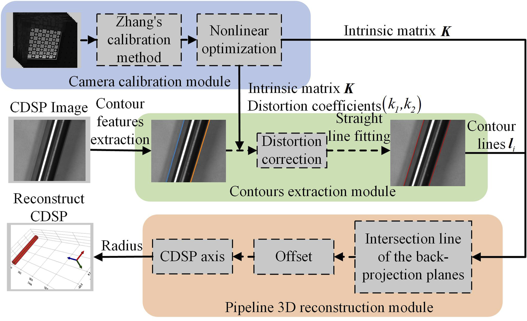
Figure 2. The rapid 3D reconstruction method process of CDSP.

The above process includes camera calibration module, contours extraction module, and pipeline 3D reconstruction module. In the camera calibration module, we use $H$ checkerboard targets for calibration, and use the Zhang’s calibration method [21] to obtain the initial estimates of the camera intrinsic matrix $\mathit{K}$, the distortion coefficients $\left(k_1,k_2\right)$, and the extrinsic parameters $\left({\mathit{R}}_h^{CT},{\mathit{t}}_h^{CT}\right)$, where $\left(k_1,k_2\right)$ represents the first-order and second-order radial distortion coefficients, and $\left({\mathit{R}}_h^{CT},{\mathit{t}}_h^{CT}\right)$ represents the rotation and translation between the camera coordinate system and the target coordinate system in the $h^{th}$ calibration image. Since the radial distortion usually displayed by the camera is more obvious, and the influence of tangential distortion is relatively small. Therefore, this paper only considers the first two terms of radial distortion coefficients $\left(k_1,k_2\right)$. Then, the Levenberg Marquardt (LM) algorithm [22] is used to optimize the initial estimates to obtain more accurate $\mathit{K}$, $\left(k_1,k_2\right)$, and $\left({\mathit{R}}_h^{CT},{\mathit{t}}_h^{CT}\right)$. In the contours extraction module, we first detect the contour edges of the image and extract contour features, then correct the distortion of contour feature points using the $\mathit{K}$ and $\left(k_1,k_2\right)$ obtained from the camera calibration module, and finally fit the contour feature points with straight lines based on the least square method to obtain the contour lines ${\mathit{l}}_i$ in the CDSP image. The pipeline 3D reconstruction module calculates the pose of the CDSP axis. Firstly, we use the ${\mathit{l}}_i$ obtained from the contours extraction module as input, and combine the $\mathit{K}$ obtained from the camera calibration module to calculate the back-projection planes ${\mathit{\pi }}_i$. By the normal vectors ${\mathit{n}}_i$ of ${\mathit{\pi }}_i$, we obtain the direction vector ${\mathit{v}}_{\mathit{L}}$ of the intersection line $\mathit{L}$ between ${\mathit{\pi }}_1$ and ${\mathit{\pi }}_2$. Then, after calculating the offset direction ${\mathit{v}}_{\mathit{O}{\mathit{P}}_{\mathit{C}}}$ and offset distance $d_{\mathit{O}{\mathit{P}}_{\mathit{C}}}$, we can obtain the three-dimensional coordinate of point ${\mathit{P}}_{\mathit{C}}$ in the world coordinate system. Finally, the 3D pose of the CDSP axis can be determined by point ${\mathit{P}}_{\mathit{C}}$ and direction vector ${\mathit{v}}_{\mathit{L}}$.

3.1 Camera calibration module

Camera calibration is a fundamental issue in visual technology, a key step in linking 2D image information with 3D spatial information, and a necessary condition for 3D reconstruction. The checkerboard target is not only easy to make, but also provides rich and easily detectable feature points in the image. Therefore, this article uses a checkerboard target with clear corner features for calibration. The parameters that need to be calibrated include the camera intrinsic matrix $\mathit{K}$, the distortion coefficients $\left(k_1,k_2\right)$, and the extrinsic parameters $\left({\mathit{R}}_h^{CT},{\mathit{t}}_h^{CT}\right)$. Firstly, randomly place a flat checkerboard target in the public field of view, and ensure that the size and position of the target can cover most of the camera’s field of view, in order to collect sufficient calibration data. Capture calibration images at different positions from the same perspective by moving the target. Afterwards, we use the camera calibration method proposed by Zhang [21] to obtain the initial estimates of $\mathit{K}$, $\left(k_1,k_2\right)$ and $\left({\mathit{R}}_h^{CT},{\mathit{t}}_h^{CT}\right)$. The LM algorithm [22] was used to perform nonlinear optimization on $\mathit{K}$, $\left(k_1,k_2\right)$ and $\left({\mathit{R}}_h^{CT},{\mathit{t}}_h^{CT}\right)$ through Equation 7, minimizing the reprojection error of all feature points.

$\mathcal{L}={\displaystyle \sum _{h=1}^H}{\displaystyle \sum _{j=1}^J}{‖e_{hj}-\widehat{e}\left(\mathit{K},k_1,k_2,{\mathit{R}}_h^{CT},{\mathit{t}}_h^{CT},E_j\right)‖}^2(7)$

where $E_j$ denotes the three-dimensional coordinate of the $j^{th}$ feature point in the calibration image, $\widehat{e}\left(\mathit{K},k_1,k_2,{\mathit{R}}_h^{CT},{\mathit{t}}_h^{CT},E_j\right)$ denotes the projection of $E_j$ in the $h^{th}$ calibration image, and $e_{hj}$ denotes the pixel coordinate of the $j^{th}$ feature point in the $h^{th}$ calibration image.

3.2 Contours extraction module

The edge contour of CDSP comprises circular contours of end faces and straight contours. The method presented in this paper completes 3D reconstruction based on the constraint relationship between the contour lines and the axis of CDSP. Therefore, this method does not require detecting the circular contours of end faces of CDSP and can achieve 3D reconstruction for CDSP of any length. In this paper, we use the subpixel edge detection method proposed by Trujillo-Pino [23] to obtain the pixel coordinates $\left(\breve{u},\breve{v}\right)$ of contour feature points in CDSP image. This method estimates the subpixel position of the edge by considering the partial area effects around the edge. Due to the distortion of the camera lens, the distortion coefficients $\left(k_1,k_2\right)$ obtained from the camera calibration module, and the coordinate $\left(u_0,v_0\right)$ of the principal point in the intrinsic matrix $\mathit{K}$, are used to correct the distortion of the obtained contour feature points by Equation 8.

$\left\{\begin{array}{c}\breve{u}=u+\left(u-u_0\right)\left[k_1\left(x^2+y^2\right)+k_2{\left(x^2+y^2\right)}^2\right]\\ \breve{v}=v+\left(v-v_0\right)\left[k_1\left(x^2+y^2\right)+k_2{\left(x^2+y^2\right)}^2\right]\end{array}\right.(8)$

where $\left(x,y\right)$ denotes the undistorted normalized image coordinates, and $\left(u,v\right)$ denotes the undistorted pixel coordinates.

Due to the apparent contours of CDSP in the image are two straight lines, we use the RANSAC algorithm [24] to estimate one of the straight line models by randomly selecting sample points from the contour feature points. Then, the distance from other points to this model is calculated to determine whether they belong to the model’s feature points. After selecting the points that comply, we obtain the feature points set $\left\{\left(u_g^{\prime },v_g^{\prime }\right)\left|g\in 1,\dots ,G\right.\right\}$ of the straight line model, where $\left(u_g^{\prime },v_g^{\prime }\right)$ denotes the pixel coordinates of the feature points in this model. Among the remaining feature points, the RANSAC algorithm [24] is used again to sift the feature points of another straight line model and obtain a feature points set $\left\{\left(u_m^{″},v_m^{″}\right)\left|m\in 1,\dots ,M\right.\right\}$, where $\left(u_m^{″},v_m^{″}\right)$ denotes the pixel coordinates of the feature points in the other straight line model. For CDSP images with complex backgrounds, we can also obtain the contour feature point sets of CDSP through manual filtering methods. Finally, based on the least squares method, the feature point sets in the two straight line models are fitted separately. The equations for fitting lines ${\mathit{l}}_1$ and ${\mathit{l}}_2$ are expressed in Equation 9.

$\left\{\begin{array}{l}{\mathit{l}}_1:a^{\prime }{u}_g^{\prime }+b^{\prime }{v}_g^{\prime }+c^{\prime }=0\\ {\mathit{l}}_2:a^{″}{u}_m^{″}+b^{\prime }{v}_m^{″}+c^{″}=0\end{array}\right.(9)$

where $a^{\prime },b^{\prime },c^{\prime }$ denote the coefficients of the equation of the fitting straight line ${\mathit{l}}_1$, and $a^{″},b^{″},c^{″}$ denote the coefficients of the equation of the fitting straight line ${\mathit{l}}_2$. The system of equations, which is constructed using the homogeneous coordinates of the feature points of the ${\mathit{l}}_1$ model as the coefficient matrix, is expressed as,

$\left[\begin{array}{ccc}{u}_1^{\prime }& v_1^{\prime }& 1\\ ⋮& ⋮& ⋮\\ u_G^{\prime }& v_G^{\prime }& 1\end{array}\right]\left[\begin{array}{c}{a}^{\prime }\\ b^{\prime }\\ c^{\prime }\end{array}\right]=0(10)$

Similarly, the system of equations, which is constructed using the homogeneous coordinates of the feature points of the ${\mathit{l}}_2$ model as the coefficient matrix, is expressed as,

$\left[\begin{array}{ccc}{u}_1^{″}& v_1^{″}& 1\\ ⋮& ⋮& ⋮\\ u_M^{″}& v_M^{″}& 1\end{array}\right]\left[\begin{array}{c}{a}^{″}\\ b^{″}\\ c^{″}\end{array}\right]=0(11)$

For the above two systems of equations, the eigenvector corresponding to the smallest eigenvalue of the coefficient matrix represents the least squares solution of the equations. Alternatively, we can perform SVD decomposition on the coefficient matrix and then take the vector in the right singular matrix that corresponds to the smallest singular value as the optimal solution. After solving from Equation 10 and Equation 11, we can obtain two contour lines ${\mathit{l}}_i$ in the CDSP image.

3.3 Pipeline 3D reconstruction module

In this section, based on the geometric constraints provided by the perspective projection imaging model of CDSP, the process of solving the axis 3D pose using the contour lines of CDSP in the image as input is derived. According to the contour lines ${\mathit{l}}_i$ obtained from the contours extraction module, the back-projection planes ${\mathit{\pi }}_i$ can be expressed in Equation 12.

${\mathit{\pi }}_i={\mathit{K}}^T{\mathit{l}}_i(12)$

where $T$ denotes vector transpose. Due to ${\mathit{n}}_i\perp \mathit{L}$, the direction vector ${\mathit{v}}_{\mathit{L}}$ of $\mathit{L}$ can be obtained through Equation 1. In addition, since ${\mathit{n}}_m\perp \overrightarrow{\mathit{O}{\mathit{P}}_{\mathit{C}}}$, ${\mathit{n}}_m\perp \mathit{L}$, and $\overrightarrow{\mathit{O}{\mathit{P}}_{\mathit{C}}}\perp \mathit{L}$, the direction vector ${\mathit{v}}_{\mathit{O}{\mathit{P}}_{\mathit{C}}}$ of $\overrightarrow{\mathit{O}{\mathit{P}}_{\mathit{C}}}$ can be obtained by Equation 3. Based on the ${\mathit{v}}_{\mathit{L}}$ obtained from Equation 1 and the ${\mathit{n}}_m$ obtained from Equation 2, ${\mathit{v}}_{\mathit{O}{\mathit{P}}_{\mathit{C}}}$ obtained from Equation 3 can be expressed as,

${\mathit{v}}_{\mathit{O}{\mathit{P}}_{\mathit{C}}}=\frac{{\mathit{n}}_1\times {\mathit{n}}_2}{‖{\mathit{n}}_1\times {\mathit{n}}_2‖}\times \left(\frac{{\mathit{n}}_1}{‖{\mathit{n}}_1‖}+\frac{{\mathit{n}}_2}{‖{\mathit{n}}_2‖}\right)(13)$

Since $\alpha$ is the angle between the planes ${\mathit{\pi }}_1$ and ${\mathit{\pi }}_2$, and also the angle between the normal vectors ${\mathit{n}}_1$ and ${\mathit{n}}_2$, the angle $\alpha$ obtained by Equation 4 is,

$\alpha ={\cos }^{-1}\left(\frac{{\mathit{n}}_1·{\mathit{n}}_2}{‖{\mathit{n}}_1·{\mathit{n}}_2‖}\right)(14)$

Besides, since the radius $r$ of the cross section circle $\mathit{C}$ is known and the angle $\alpha$ is obtained from Equation 14, the distance $d_{\mathit{O}{\mathit{P}}_{\mathit{C}}}$ between point $\mathit{O}$ and point ${\mathit{P}}_{\mathit{C}}$ can be obtained through Equation 5. can be expressed as,

$d_{\mathit{O}{\mathit{P}}_{\mathit{C}}}=\frac{r}{\sin \left(\left[{\cos }^{-1}\left(\frac{{\mathit{n}}_1·{\mathit{n}}_2}{‖{\mathit{n}}_1·{\mathit{n}}_2‖}\right)\right]/2\right)}(15)$

According to the distance $d_{\mathit{O}{\mathit{P}}_{\mathit{C}}}$ obtained from Equation 15 and the ${\mathit{v}}_{\mathit{O}{\mathit{P}}_{\mathit{C}}}$ obtained from Equation 13, the three-dimensional coordinate of point ${\mathit{P}}_{\mathit{C}}$ in the world coordinate system obtained from Equation 6 can be expressed as,

${\mathit{P}}_{\mathit{C}}=\frac{r}{\sin \left(\left[{\cos }^{-1}\left(\frac{{\mathit{n}}_1·{\mathit{n}}_2}{‖{\mathit{n}}_1·{\mathit{n}}_2‖}\right)\right]/2\right)}·\frac{\frac{{\mathit{n}}_1\times {\mathit{n}}_2}{‖{\mathit{n}}_1\times {\mathit{n}}_2‖}\times \left(\frac{{\mathit{n}}_1}{‖{\mathit{n}}_1‖}+\frac{{\mathit{n}}_2}{‖{\mathit{n}}_2‖}\right)}{‖\frac{{\mathit{n}}_1\times {\mathit{n}}_2}{‖{\mathit{n}}_1\times {\mathit{n}}_2‖}\times \left(\frac{{\mathit{n}}_1}{‖{\mathit{n}}_1‖}+\frac{{\mathit{n}}_2}{‖{\mathit{n}}_2‖}\right)‖}(16)$

where ${\mathit{n}}_1={\mathit{K}}^T{\mathit{l}}_1$, ${\mathit{n}}_2={\mathit{K}}^T{\mathit{l}}_2$.

Based on the above derivation, under the premise that the radius $r$ is known, taking the contour lines in the CDSP image as input, the 3D pose of the CDSP axis can be determined by the direction vector ${\mathit{v}}_{\mathit{L}}$ obtained from Equation 1 and the 3D coordinate of point ${\mathit{P}}_{\mathit{C}}$ obtained from Equation 16.

4 Experiments

To verify the effectiveness of the rapid 3D reconstruction method of CDSP, this section will conduct simulation experiment and real experiment. Specifically, the simulation experiment is designed to validate the correctness of the method, while the real experiment is aimed at verifying the feasibility of the method. This article uses a computer equipped with Intel Core i5-8250U CPU and 8 GB RAM for experiments, and uses time-consuming for 3D reconstruction as the speed evaluation metric. In the simulation experiment, we reconstruct a pipe and calculate the root mean square error (RMSE) between the distance from each point in the reconstructed pipe axis to the ideal axis and the true distance $d=0\text{mm}$. In the real experiment, we reconstruct two parallel pipes with a known true distance $d$, and calculate the RMSE between the distance from each point in the axis of one reconstructed pipe to the axis of the other reconstructed pipe and the true distance $d$. Using RMSE as the evaluation metric of accuracy, the calculation formula is expressed as,

$\text{RMSE}=\sqrt{\frac{1}{N}{\displaystyle \sum _{n=1}^N}{\left(d-d_n\right)}^2}(17)$

where $N$ denotes the number of points in the reconstructed pipe axis. In the simulation experiment, $d_n$ denotes the distance from a point in the reconstructed pipe axis to the ideal axis. In the real experiment $d_n$ denotes the distance from a point in the reconstructed pipe axis to another reconstructed pipe axis.

Assuming ${\mathit{P}}_n$ is a point in the reconstructed pipe axis. In the simulation experiment, $\mathit{Q}$ is any point in the ideal axis, and $\mathit{v}$ is the direction vector of the ideal axis. In the real experiment, $\mathit{Q}$ is any point in the axis of another reconstructed pipe, and $\mathit{v}$ is the direction vector of the axis of another reconstructed pipe. The direction vector expression from point ${\mathit{P}}_n$ to point $\mathit{Q}$ is,

$\overrightarrow{{\mathit{P}}_n\mathit{Q}}={\mathit{P}}_n-\mathit{Q}(18)$

A parallelogram is formed with $\overrightarrow{{\mathit{P}}_n\mathit{Q}}$ and the direction vector $\mathit{v}$ as adjacent sides, and the area $S$ of the parallelogram can be expressed as,

$S=‖\overrightarrow{{\mathit{P}}_n\mathit{Q}}\times \mathit{v}‖(19)$

Meanwhile, according to the parallelogram area formula, the area $S$ can also be expressed as,

$S=‖\mathit{v}‖·d_n(20)$

Combining Equation 18, Equation 19 and Equation 20, the distance $d_n$ can be expressed in Equation 21.

$d_n=\frac{‖\overrightarrow{{\mathit{P}}_n\mathit{Q}}\times \mathit{v}‖}{‖\mathit{v}‖}=\frac{‖\left({\mathit{P}}_n-\mathit{Q}\right)\times \mathit{v}‖}{‖\mathit{v}‖}(21)$

4.1 Simulation experiment

In this part, the proposed method is tested on simulated data. The cell size is set as $\left({∆}_u,{∆}_v\right)=\left(0.00345,0.00345\right)\text{mm}$, the focal length is set as $f=12\text{mm}$, the image size is set as $\left(N_u,N_v\right)=\left(2448,2048\right)$ pixel, and the coordinate of principal point is set as $\left(u_0,v_0\right)=\left(N_u/2,N_v/2\right)$, then the camera intrinsic matrix can be expressed in Equation 22.

$\mathit{K}=\left[\begin{array}{ccc}f/{∆}_u& 0& N_u/2\\ 0& f/{∆}_v& N_v/2\\ 0& 0& 1\end{array}\right](22)$

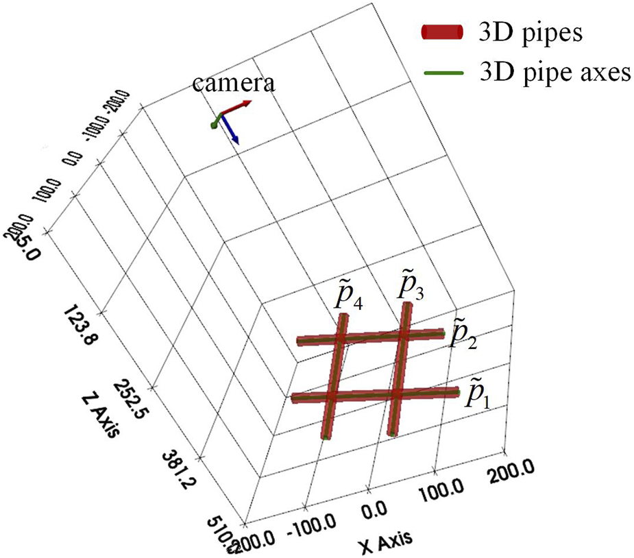
In addition, the radius and length of CDSP are set as $8\text{mm}$ and $500\text{mm}$ respectively. The experimental scene is shown in Figure 3. We establish the world coordinate system $O_W-X_W{Y}_W{Z}_W$ in the scene, and place a CDSP in the plane $Z_W=0\text{mm}$. We denote the CDSP with its center located at the origin $O_W$ and its axis parallel to the $X_W$ axis as $p_1$, and the CDSP obtained by translating $p_1$ along the positive direction of $Y_W$ as $p_2$, as shown in Figure 3A. Similarly, we denote the CDSP with its center located at the origin $O_W$ and its axis parallel to the $Y_W$ axis as $p_3$, and the CDSP obtained by translating $p_3$ along the positive direction of $X_W$ as $p_4$, as illustrated in Figure 3B. The optical center $O_C$ is located at the world coordinate system $\left(-150,-200,-300\right)\text{mm}$ and points to $O_W$.

Figure 3

Figure 3. The scene of simulation experiment. (A) The experimental scene of $p_1$ and $p_2$, (B) The experimental scene of $p_3$ and $p_4$.

Based on the scene of the above simulation experiment, The images of $p_1$, $p_2$, $p_3$ and $p_4$ generated from simulated data are shown in Figure 4.

Figure 4

Figure 4. The images generated from simulation data.

In order to verify the correctness of the proposed method, the projected contour lines of CDSP are obtained from the simulated data through the cylindrical target perspective projection model [25]. Then, we use the proposed method to achieve 3D reconstruction of four pipes $p_1$, $p_2$, $p_3$ and $p_4$. The final experimental results are shown in Figure 5. Figure 5 displays the 3D pipes reconstructed using the proposed method, as well as the true 3D pipes generated using simulated data. It can be seen that the reconstructed 3D pipes completely overlap with the true 3D pipes.

Figure 5

Figure 5. 3D reconstruction effects of simulation experiment.

In order to consider the impact of radius measurement errors on reconstruction, we set the radius measurement errors to $\pm 0.02\text{mm}$, $\pm 0.05\text{mm}$, and $\pm 0.10\text{mm}$ respectively, and then conducted experiments with radius measurement values containing errors. After completing the reconstruction, we calculated the RMSE using Equation 17, and the calculation results are shown in Table 1. It can be seen from the table that when the radius measurement errors are ±0.02mm, ±0.05mm, and ±0.10mm, the average RMSEs are 0.944mm, 2.361mm, and 4.721mm, respectively. As the radius measurement error increases, the accuracy of reconstruction gradually decreases.

Table 1

Table 1. Comparison of the impact of radius measurement errors.

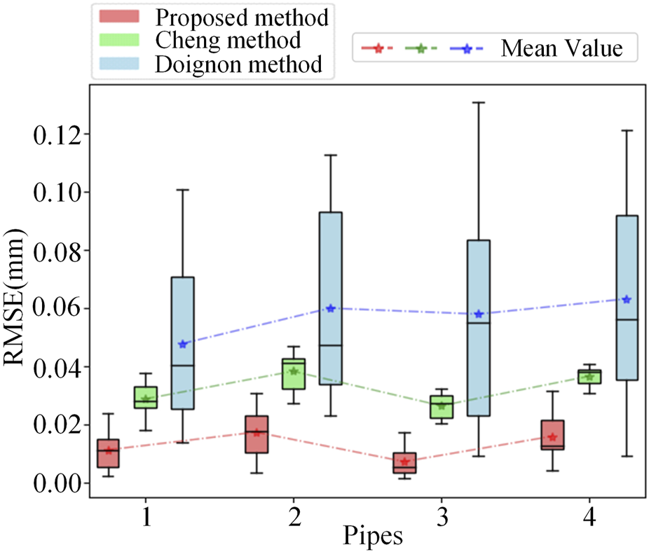
In addition, in order to approach the actual experimental conditions more closely, we add gaussian random noise with a mean of 0 and a noise level of 0.1 to the contour feature points, and then conduct a comparison experiment in terms of accuracy and speed using the Doignon [19] method, the Cheng [20] method, and the proposed method respectively. In the accuracy comparison experiment, each method was tested 10 times and the RMSE was calculated using Equation 17. The calculation results are shown in Figure 6. Figure 6 displays the RMSE for 10 reconstructions of each pipe using three different methods, as well as the average RMSE over the 10 times. The average RMSE for reconstructing the four pipes using the proposed method is 0.013mm, while the average RMSE for the Doignon [19] method is 0.057mm, and the average RMSE for the Cheng [20] method is 0.033 mm. Compared with the other two methods, the RMSE of the proposed method is the lowest, which also indicates that the proposed method is less sensitive to noise. This is because the proposed method adopts simple straight line fitting model, which has low sensitivity to noise. The Cheng [20] method affects the matching accuracy of the coupled point pairs due to noise, which in turn affects the accuracy of the reconstruction results. The Doignon [19] method uses curve model for fitting, and its parameter estimation is easily affected by noise, which in turn affects the accuracy of pose parameters. Compared with the other two methods, the proposed method is faster and less sensitive to noise. In terms of applicability, Cheng [20] method can achieve 3D reconstruction of constant-diameter pipelines, while the proposed method and Doignon [19] method are only applicable to 3D reconstruction of constant-diameter straight pipelines. This is a potential drawback of the method proposed in this article and also an area for improvement in our future work.

Figure 6

Figure 6. Comparison of experimental reconstruction accuracy.

Afterwards, we calculate the time taken by the three methods to complete the reconstruction of pipes $p_1$, $p_2$, $p_3$ and $p_4$ respectively, and the results are shown in Table 2. Table 2 displays the time taken to complete the reconstruction of each pipe with three methods separately, and take the average of the time taken to reconstruct four pipes as the time-consuming of each method. The time-consuming of the proposed method is $9.984\times {10}^{-4}\mathrm{s}$, while the Doignon [19] method and Cheng [20] method are $2.451\mathrm{s}$ and $2.367\mathrm{s}$ respectively. The time-consuming for reconstructing each pipe by the proposed method is less than that of the other two methods, and there is a significant increase in reconstruction speed. This is because the straight line fitting used in the proposed method is mainly based on solving linear equations, and the computational complexity is relatively small. The Doignon [19] method uses curve fitting with equations containing multiple coefficients, and the solving process involves nonlinear operations. The Cheng [20] method requires finding the coupled point pairs for each cross section circle, making the reconstruction process cumbersome. Through the comparison of accuracy and speed experiments, we have verified the correctness of the proposed method and can achieve rapid 3D reconstruction of CDSP.

Table 2

Table 2. Comparison of experimental reconstruction time-consuming.

To test the noise resistance of the proposed method in this article, we added Gaussian noise with an average value of 0 and a standard deviation range of 0 to 3 pixel (step size of 0.2 pixel) to the feature point coordinates of the synthesized image, and conducted 10 independent experiments for each noise level. Calculate the RMSE for different noise levels after completing the reconstruction. The RMSE for each noise level is shown in Figure 7. As can be seen from Figure 7, the accuracy gradually decreases with the increase of noise level, and it has a linear relationship with the noise level. When the accuracy requirement reaches 0.2mm, 1.5 pixel of noise can be tolerated. When the accuracy requirement reaches 0.4mm, 3 pixel of noise can be tolerated.

Figure 7

Figure 7. The influence of different noise levels on reconstruction accuracy.

4.2 Real experiment

The above simulation experiment has verified the correctness of the proposed method. In order to further verify the feasibility of the proposed method, this section will conduct real experiment based on real data. The camera used in the experiment is Daheng MER-503-23 GM-P camera with resolution of $2448\times 2048$ pixels, equipped with HN-P-1628-6M-C2/3 lens with focal length of $16\text{mm}$. We set up a real experimental scene that is consistent with the scene of simulation experiment as shown in Figure 8A. When the CDSP is placed at two different positions in the scene, they are denoted as ${\stackrel{\sim }{p}}_1$ and ${\stackrel{\sim }{p}}_3$ respectively. By translating ${\stackrel{\sim }{p}}_1$ and ${\stackrel{\sim }{p}}_3$ separately, we obtain ${\stackrel{\sim }{p}}_2$ and ${\stackrel{\sim }{p}}_4$. Since there is no true value in the real experiment, we use the distance of pipe translation as the true distance $d$ in Equation 17. Measured by a vernier caliper with an accuracy of $0.02\text{mm}$, the diameter and length of CDSP are $16\text{mm}$ and $300\text{mm}$ respectively, the distance between the two support columns of ${\stackrel{\sim }{p}}_1$ and ${\stackrel{\sim }{p}}_2$ is $112.67\text{mm}$, the distance between the two support columns of ${\stackrel{\sim }{p}}_3$ and ${\stackrel{\sim }{p}}_4$ is $112.68\text{mm}$, and the diameter of the support column is $12.68\text{mm}$. Based on this, we can calculate that the translation distances for pipes ${\stackrel{\sim }{p}}_1$ and ${\stackrel{\sim }{p}}_3$ are $99.99\text{mm}$ and $100.00\text{mm}$ respectively.

Figure 8

Figure 8. (A) The scene of real experiment, (B) The images collected in the experiment, (C) The images with contour lines and projected axis.

Based on the scene of the above real experiment, we first calibrate the camera used in the experiment. The calibration parameters obtained using the method in the camera calibration module are shown in Table 3.

Table 3

Table 3. Camera calibration results.

Then, we collect images of ${\stackrel{\sim }{p}}_1$, ${\stackrel{\sim }{p}}_2$, ${\stackrel{\sim }{p}}_3$ and ${\stackrel{\sim }{p}}_4$ respectively, and the collected images are shown in Figure 8B. After feature extraction from the collected images using the method in the contours extraction module, the contour lines of ${\stackrel{\sim }{p}}_1$, ${\stackrel{\sim }{p}}_2$, ${\stackrel{\sim }{p}}_3$ and ${\stackrel{\sim }{p}}_4$ in the image are obtained. Subsequently, taking the obtained contour lines as input, the pose of each pipe axis is calculated using the method in the pipeline 3D reconstruction module. The contour lines and projected axes are shown in Figure 8C. Finally, the reconstructed 3D effects of ${\stackrel{\sim }{p}}_1$, ${\stackrel{\sim }{p}}_2$, ${\stackrel{\sim }{p}}_3$ and ${\stackrel{\sim }{p}}_4$ based on the collected images are shown in Figure 9. Figure 9 displays the reconstructed 3D pipes and their axes from the above images.

Figure 9

Figure 9. 3D reconstruction effects of real experiment.

In addition, based on the scene of the above real experiment, we collect five groups of images for ${\stackrel{\sim }{p}}_1$ and ${\stackrel{\sim }{p}}_2$, and another five groups of images for ${\stackrel{\sim }{p}}_3$ and ${\stackrel{\sim }{p}}_4$. Afterwards, we use the proposed method, the Doignon [19] method, and Cheng [20] method to perform 3D reconstruction on these 10 groups of images. The reconstruction error results of one group of ${\stackrel{\sim }{p}}_1$, ${\stackrel{\sim }{p}}_2$ and one group of ${\stackrel{\sim }{p}}_3$, ${\stackrel{\sim }{p}}_4$ are shown in Figure 10. In Figure 10, the x-axis represents the point number, and the y-axis represents the error of each point. Figure 10A displays the distance deviation of each point on the reconstructed axis of ${\stackrel{\sim }{p}}_1$ to the reconstructed axis of ${\stackrel{\sim }{p}}_2$, and Figure 10B displays the distance deviation of each point on the reconstructed axis of ${\stackrel{\sim }{p}}_3$ to the reconstructed axis of ${\stackrel{\sim }{p}}_4$. Meanwhile, the reconstruction time-consuming for the set of ${\stackrel{\sim }{p}}_1$, ${\stackrel{\sim }{p}}_2$ and the set of ${\stackrel{\sim }{p}}_3$, ${\stackrel{\sim }{p}}_4$ are shown in Table 4.

Figure 10

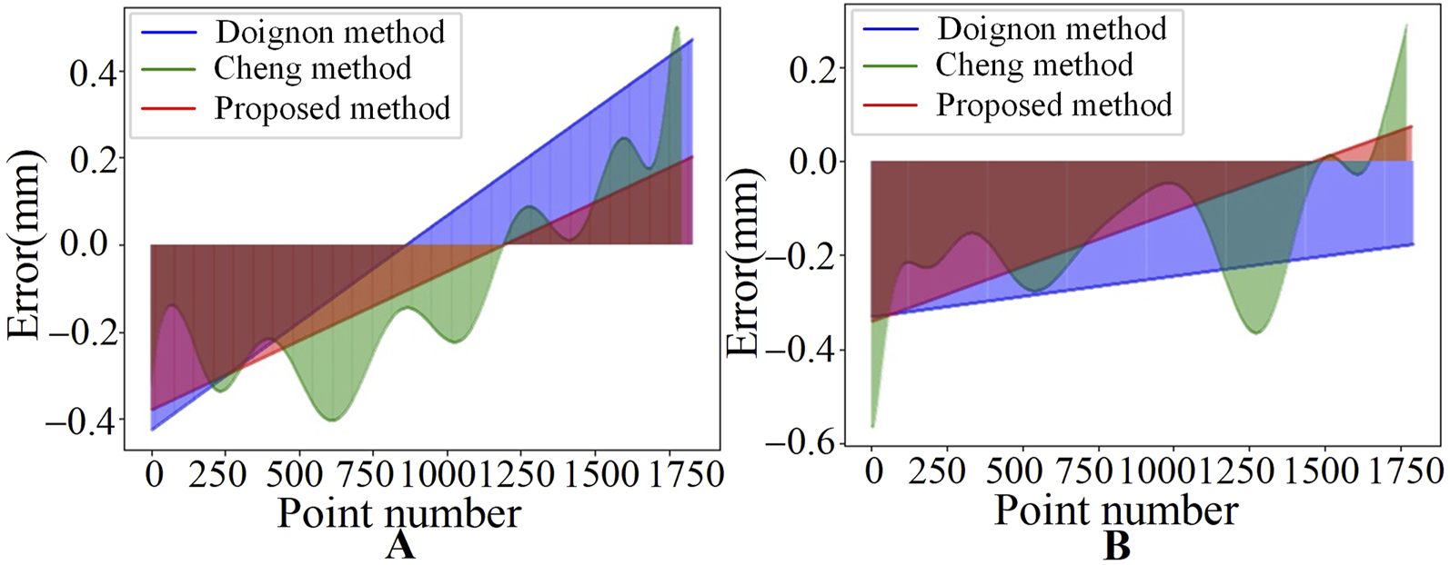
Figure 10. Comparison of reconstruction error results for one group of experiments. (A) The reconstruction error results for ${\stackrel{\sim }{p}}_1$ and ${\stackrel{\sim }{p}}_2$, (B) The reconstruction error results for ${\stackrel{\sim }{p}}_3$ and ${\stackrel{\sim }{p}}_4$.

Table 4

Table 4. Comparison of reconstruction time-consuming for one group of experiments.

After completing the 3D reconstruction of 10 groups of images using three different methods, we calculate the RMSE of each group using Equation 17. Meanwhile, we calculate the time taken to complete the reconstruction for each pipe and used the average of the time taken to complete the reconstruction for the two pipes as the time-consuming for each group of experiments. In the experimental results shown in Figure 11, the x-axis represents the group number, and the y-axis shows the RMSE of the reconstructed pipe for each group and the average time-consuming to complete the pipe reconstruction for each group. The average RMSE for the 10 groups using the proposed method is $0.165\text{mm}$, and the average time-consuming is $1.917\times {10}^{-3}\mathrm{s}$. The average RMSE of the Doignon [19] method is $0.314\text{mm}$, with the average time-consuming of $2.034\mathrm{s}$. The average RMSE of the Cheng [20] method is $0.180\text{mm}$, with the average time-consuming of $2.071\mathrm{s}$. The accuracy of the proposed method is similar to Cheng [20] method and slightly higher than Doignon [19] method, and the time-consuming of the proposed method is the least. In the real experiment, the three-dimensional reconstruction accuracy of the pipe axis is affected by many factors such as camera calibration accuracy, lens distortion, edge contour extraction accuracy, image noise, etc., resulting in the improvement of accuracy is not as obvious as that of the simulation experiment. The obvious advantage of the proposed method compared to the three methods is the improvement in speed. The comparison results of accuracy and speed are consistent with the simulation experiment, proving that proposed method can effectively achieve rapid 3D reconstruction of CDSP.

Figure 11

Figure 11. Comparison of experimental results among all groups.

To discuss the robustness of the proposed method under different lighting conditions and backgrounds, we collected CDSP images under different lighting conditions and backgrounds for experiments. For more complex scenes, we use manual filtering to extract contour features, and then use the proposed method for reconstruction. The collected images and their reconstructed effects are shown in Figure 12. Figure 12A shows the collected CDSP images, and Figure 12B shows the 3D reconstruction effect of CDSP. From the experimental results, it can be seen that the method proposed in this paper can effectively achieve 3D reconstruction of CDSP under different lighting conditions and backgrounds, provided that the contour features can be accurately extracted.

Figure 12

Figure 12. Collected CDSP images and their reconstruction effects. (A) the collected CDSP images, (B) the 3D reconstruction effect of CDSP.

5 Conclusion

This paper proposes a rapid 3D reconstruction method of CDSP based on the single-view perspective projection imaging model to address the inefficiency of 3D pipeline reconstruction in tasks such as positioning and navigation for pipeline inspection drones and pipeline surface defect detection. This method first establishes a single-view perspective projection imaging model of CDSP, and under the premise of known radius, the geometric constraints of this model provide a direct method to solve the 3D pose of the CDSP axis. Subsequently, the results of the simulation experiment indicate that the reconstructed pipeline overlaps with the simulated pipeline, and under low noise conditions in the simulated images, the proposed method achieves an average reconstruction accuracy of $0.013\text{mm}$, with an average time-consuming of $9.984\times {10}^{-4}\mathrm{s}$. The results of the real experiment show that the average reconstruction accuracy of the proposed method is $0.165\text{mm}$, with an average time-consuming of $1.917\times {10}^{-3}\mathrm{s}$. While the accuracy is similar to traditional methods, the speed is improved by $99.907\%$, demonstrating that this method can effectively achieve rapid 3D reconstruction of CDSP, and has application value in tasks such as positioning and navigation for pipeline inspection drones and pipeline surface defect detection.

Data availability statement

The raw data supporting the conclusions of this article will be made available by the authors, without undue reservation.

Author contributions

JY: Conceptualization, Formal Analysis, Methodology, Visualization, Writing–original draft. XC: Conceptualization, Funding acquisition, Methodology, Project administration, Writing–review and editing. HT: Methodology, Supervision, Writing–review and editing. XL: Supervision, Writing–review and editing. HZ: Methodology, Writing–review and editing.

Funding

The author(s) declare that financial support was received for the research, authorship, and/or publication of this article. This research was supported by the National Natural Science Foundation of China (62201151, 62271148).

Conflict of interest

The authors declare that the research was conducted in the absence of any commercial or financial relationships that could be construed as a potential conflict of interest.

Publisher’s note

All claims expressed in this article are solely those of the authors and do not necessarily represent those of their affiliated organizations, or those of the publisher, the editors and the reviewers. Any product that may be evaluated in this article, or claim that may be made by its manufacturer, is not guaranteed or endorsed by the publisher.

References

1. Wu Y, Gao L, Chai J, Li Z, Ma C, Qiu F, et al. Overview of health-monitoring technology for long-distance transportation pipeline and progress in DAS technology application. Sensors (2024) 24(2):413. doi:10.3390/s24020413

PubMed Abstract | CrossRef Full Text | Google Scholar

2. Nguyen HH, Park JH, Jeong HY. A simultaneous pipe-attribute and PIG-Pose estimation (SPPE) using 3-D point cloud in compressible gas pipelines. Sensors (2023) 23(3):1196. doi:10.3390/s23031196

PubMed Abstract | CrossRef Full Text | Google Scholar

3. Lyu F, Zhou X, Ding Z, Qiao X, Song D. Application research of ultrasonic-guided wave technology in pipeline corrosion defect detection: a review. Coatings (2024) 14(3):358. doi:10.3390/coatings14030358

CrossRef Full Text | Google Scholar

4. Cirtautas D, Samaitis V, Mažeika L, Raišutis R, Žukauskas E. Selection of higher order lamb wave mode for assessment of pipeline corrosion. Metals (2022) 12(3):503. doi:10.3390/met12030503

CrossRef Full Text | Google Scholar

5. Hussain M, Zhang T, Chaudhry M, Jamil I, Kausar S, Hussain I. Review of prediction of stress corrosion cracking in gas pipelines using machine learning. Machines (2024) 12(1):42. doi:10.3390/machines12010042

CrossRef Full Text | Google Scholar

6. Chen X, Zhu X, Liu C. Real-time 3D reconstruction of UAV acquisition system for the urban pipe based on RTAB-Map. Appl Sci (2023) 13(24):13182. doi:10.3390/app132413182

CrossRef Full Text | Google Scholar

7. Cheng X, Zhong B, Tan H, Qiao J, Yang J, Li X. Correction for geometric distortion in the flattened representation of pipeline external surface. Eng Res Express (2024) 6(2):025218. doi:10.1088/2631-8695/ad4cb1

CrossRef Full Text | Google Scholar

8. Varady T, Martin RR, Cox J. Reverse engineering of geometric models—an introduction. Computer-aided Des (1997) 29(4):255–68. doi:10.1016/s0010-4485(96)00054-1

CrossRef Full Text | Google Scholar

9. He WM, Sato H, Umeda K, Sone T, Tani Y, Sagara M, et al. A new methodology to evaluate error space in CMM by sequential two points method. In: Mechatronics for safety, security and dependability in a new era. Elsevier (2007). p. 371–6. doi:10.1016/B978-008044963-0/50075-8

CrossRef Full Text | Google Scholar

10. Zhou L, Wu G, Zuo Y, Chen X, Hu H. A comprehensive review of vision-based 3D reconstruction methods. Sensors (2024) 24(7):2314. doi:10.3390/s24072314

PubMed Abstract | CrossRef Full Text | Google Scholar

11. Isgro F, Odone F, Verri A. An open system for 3D data acquisition from multiple sensor. In: Seventh international workshop on computer architecture for machine perception (CAMP'05). IEEE (2005) p. 52–7. doi:10.1109/camp.2005.13

CrossRef Full Text | Google Scholar

12. Huang Z, Li D. A 3D reconstruction method based on one-dimensional galvanometer laser scanning system. Opt Lasers Eng (2023) 170:107787. doi:10.1016/j.optlaseng.2023.107787

CrossRef Full Text | Google Scholar

13. Al-Temeemy AA, Al-Saqal SA. Laser-based structured light technique for 3D reconstruction using extreme laser stripes extraction method with global information extraction. Opt And Laser Technology (2021) 138:106897. doi:10.1016/j.optlastec.2020.106897

CrossRef Full Text | Google Scholar

14. Hwang S, Lee D. 3d pose estimation of catheter band markers based on single-plane fluoroscopy. In: 2018 15th international conference on ubiquitous robots (UR). IEEE (2018) p. 723–8. doi:10.1109/urai.2018.8441789

CrossRef Full Text | Google Scholar

15. Zhang L, Ye M, Chan PL, Yang GZ. Real-time surgical tool tracking and pose estimation using a hybrid cylindrical marker. Int J Comput Assist Radiol Surg (2017) 12:921–30. doi:10.1007/s11548-017-1558-9

PubMed Abstract | CrossRef Full Text | Google Scholar

16. Lee JD, Lee JY, You YC, Chen CH. Determining location and orientation of a labelled cylinder using point-pair estimation algorithm. Int J Pattern Recognition Artif Intelligence (1994) 8(01):351–71. doi:10.1142/s0218001494000176

CrossRef Full Text | Google Scholar

17. Shiu H. Pose determination of circular cylinders using elliptical and side projections. In: IEEE 1991 international conference on systems engineering. IEEE (1991) p. 265–8. doi:10.1109/icsyse.1991.161129

CrossRef Full Text | Google Scholar

18. Zhang T, Liu J, Liu S, Tang C, Jin P. A 3D reconstruction method for pipeline inspection based on multi-vision. Measurement (2017) 98:35–48. doi:10.1016/j.measurement.2016.11.004

CrossRef Full Text | Google Scholar

19. Doignon C, Mathelin MD. A degenerate conic-based method for a direct fitting and 3-d pose of cylinders with a single perspective view. In: Proceedings 2007 IEEE international conference on robotics and automation. IEEE (2007) p. 4220–5. doi:10.1109/robot.2007.364128

CrossRef Full Text | Google Scholar

20. Cheng X, Sun J, Zhou F, Xie Y. Shape from apparent contours for bent pipes with constant diameter under perspective projection. Measurement (2021) 182:109787. doi:10.1016/j.measurement.2021.109787

CrossRef Full Text | Google Scholar

21. Zhang Z. A flexible new technique for camera calibration. IEEE Trans pattern Anal machine intelligence (2000) 22(11):1330–4. doi:10.1109/34.888718

CrossRef Full Text | Google Scholar

22. Levenberg K. A method for the solution of certain non-linear problems in least squares. Q Appl Mathematics (1944) 2(2):164–8. doi:10.1090/qam/10666

CrossRef Full Text | Google Scholar

23. Trujillo-Pino A, Krissian K, Alemán-Flores M, Santana-Cedrés D. Accurate subpixel edge location based on partial area effect. Image Vis Comput (2013) 31(1):72–90. doi:10.1016/j.imavis.2012.10.005

CrossRef Full Text | Google Scholar

24. Fischler MA, Bolles RC. Random sample consensus: a paradigm for model fitting with applications to image analysis and automated cartography. Commun ACM (1981) 24(6):381–95. doi:10.1145/358669.358692

CrossRef Full Text | Google Scholar

25. Sun J, Cheng X, Fan Q. Camera calibration based on two-cylinder target. Opt Express (2019) 27(20):29319–31. doi:10.1364/OE.27.029319

PubMed Abstract | CrossRef Full Text | Google Scholar