Abstract
This paper focuses on obtaining the exact solutions to the variable-coefficient forced Korteweg-de Vries (KdV) equation for modeling spatial inhomogeneity in fluids. By combining the direct similarity reduction-based CK method with the (G'/G) expansion method, three new similarity solutions are obtained for this variable-coefficient forced KdV equation.
1 Introduction
The forced KdV equation with variable coefficients plays a crucial role in researching the waves motion and nonlinear phenonmeno [1], and it attracts more and more research attentions [2]. In this paper, we examine the forced KdV equation with variable coefficients:where is the wave function and and are scaled spatial and temporal coordinates, respectively. is a nonlinearity coefficient, is a dispersive coefficient, is a line-damping coefficient, is a dissipative coefficient, and represents the external force effect function. Under suitable selections of the coefficient functions, Equation 1.1 reduces to a sequence of integrable systems or describe the nonlinear waves in a fluid-filled tube [3], weakly nonlinear waves in the water of variable depth [4], and it models the spatial inhomogeneity in fluids [5]. The classical KdV equation was first derived from shallow water wave theory to describe the propagation of water waves in the long wave limit (surface gravity waves) [6]. The coefficients of variation in Equation 1.1 are due to geometric and physical inhomogeneities [3, 7].
In this context, we suppose that the external force effect function has the following form according to [5]:In particular, when , , , , and , H.L. Demiray [8] obtained the solitary wave solution via coordinate transformation. When , , , , and , H.L. Demiray [9] obtained a progressive wave-type solution through the reductive perturbation method. When , Zhang et al. [10] utilized the Wronskian technique and Hirota method to obtain a bilinear form and an analytic N-soliton-like solution. On the basis of symbolic computation, Tian et al. [11] obtained solutions for the Airy, Hermit and Jacobian elliptic functions [12]. Utilizing the Hirota bilinear method, Yu et al. [13] obtained an N-soliton solution and a type of analytic solution.
Various methods have been applied to search for exact solutions to nonlinear evolution equations (see [14–23]), including the expansion method [22, 24], the Hirota bilinear method [18], the inverse scattering transform method [16], the CK direct method [15], and the nonclassic Lie group method [14], among others.
In general, solving ordinary differential equations is easier than directly constructing partial differential equations. However, owing to variable coefficients, it remains difficult to solve an ordinary differential equation with variable coefficients. In the present work, first, by applying the direct similarity reduction-based CK method, we transform the partial differential equation shown in (1.1) into an ordinary differential equation. Then, solutions are obtained for the above ordinary differential equation via the expansion method. Finally, we can obtain three new similarity solutions to the variable-coefficient forced KdV equation in (1.1) and express the graphics of these similarity solutions. This equation may represent the main profile of these solutions for Equation 1.1.
2 Direct similarity reduction-based CK method
We hypothesize that the solution to Equation 1.1 takes the following form:Indeed, Equation 2.1 may represent the general form of the similarity solutions for Equation 1.1 (see [25]), and it is sufficient to consider the solutions for Equation 1.1 in the form of Equation 2.1. By substituting Equations 1.2, 2.1 into (1.1), we obtainwhere , , and . To reduce Equation 2.2 to an ordinary differential equation with respect to , the derivatives of should be only functions of and . Moreover, when conducting normalization with a coefficient of , namely, , the coefficients of must satisfywhere is a function and can be determined as follows. From Equation 2.3, we have
After an integration step, we obtainwhere is the integral function. Letting , we have
After an integration process, we obtainwhere is the function generated via integration. Let ; from Equation 2.4, we have thatLetting , , and , we have
Next, we compute , , and . By substituting Equation 2.5 into Equation 2.2, we deduce that
For the above equation to reduce to a solvable equation with respect to , the ratios of the coefficients and the derivatives of the equation must be dependent on alone. This condition provides the relationships for , , and , ensuring that any solution is a similarity reduction solution. Then, we introduce the following three footnotes (see [15]).
Remark 1We adopt the coefficient of (i.e., ) as the normalizing factor and thus impose the condition that the other coefficients must take the form , where is a function of that needs to be determined.
Remark 2Uppercase Greek letters are reserved for undetermined functions of , ensuring that after performing operations (such as differentiation, integration, exponentiation, and rescaling), the result can still be denoted by the same letter. For example, the derivative of is denoted as .
Remark 3
Three degrees of freedoms exist in the determination of
,
,
and
and can be exploited (without loss of generality) to keep the proposed method manageable:
(i) if is expressed as , we can simplify it by setting , which is equivalent to performing the substitution ;
(ii) if is expressed as , we can simplify it by setting , which is equivalent to performing the substitution ];
(iii) if is determined by an equation with the form , where is any invertible function, then we can take [by substituting ].
The following exact solution forms exist for
Equation 2.22, and they can be acquired by substituting
Equation 2.26into
Equation 2.24.
Case 1.If , then
Case 2.If , then
Case 3. If , then
3 Conclusion
Substitute
Equation 2.27–
2.29into
Equation 2.23and the following forms of similarity solutions exist for
Equation 1.1.
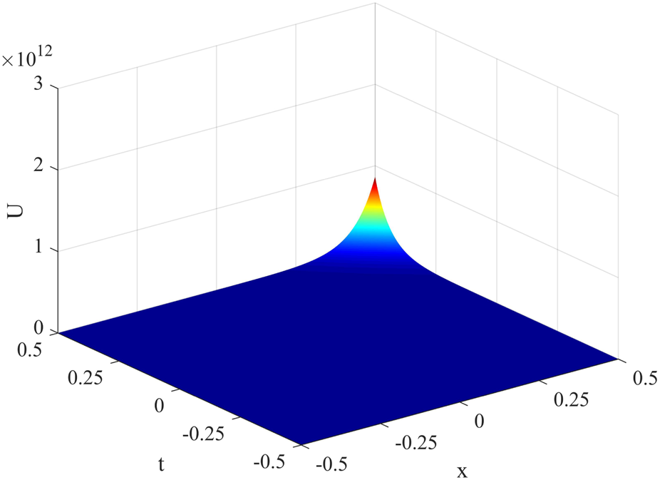
Case 1. If , then
The similar solution corresponding to Case 1 is expressed in Figure 1.
FIGURE 1

The values determined for u1(x, t) when λ = 1, μ = −1, A1 = 100, A2 = A = B = A0 = B0 = a(t) = b(t) = d(t) = 1.
The values determined for when .
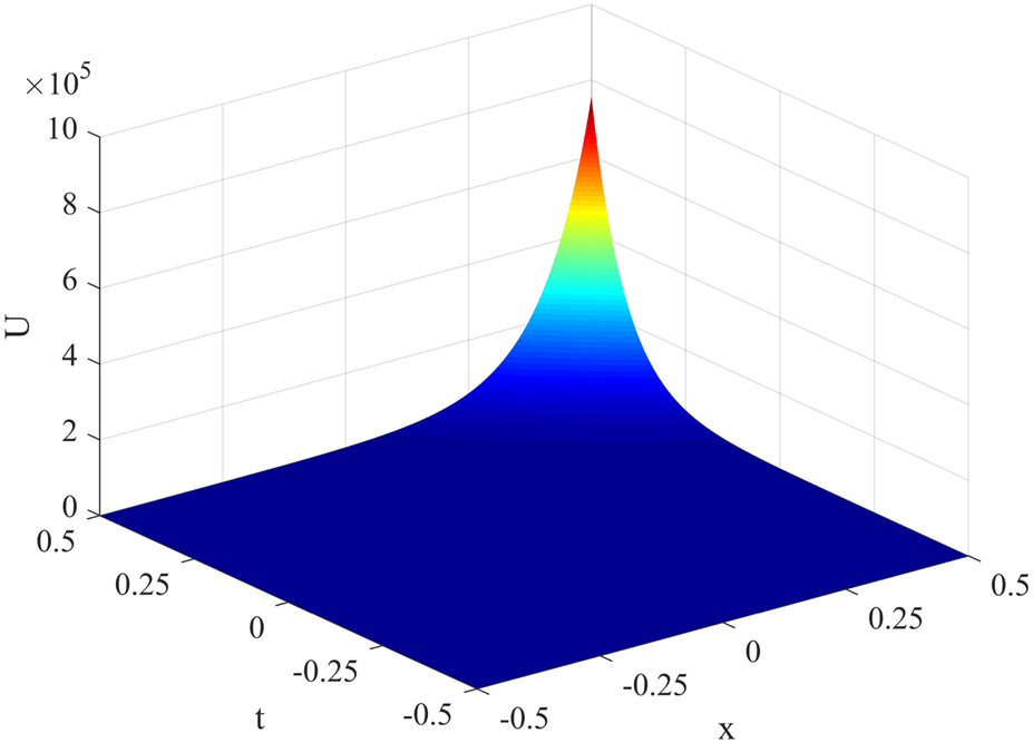
Case 2. If , then
The similar solution corresponding to Case 2 is expressed in Figure 2.
FIGURE 2
The values determined for u2(x, t) when λ = 1, μ = 1, A1 = 100, A2 = A = B = A0 = B0 = a(t) = b(t) = d(t) = 1.
The values determined for
when
.
Case 3. If , then
The similar solution corresponding to Case 3 is expressed in Figure 3.
FIGURE 3
The values determined for u3(x, t) when λ = 2, A1 = 100, μ = A2 = A = B = A0 = B0 = a(t) = b(t) = d(t) = 1.
The values determined for when .
According to the above discussion, the shape of the graphic is sensitive to the values of and . Indeed, we can clearly see the change trends exhibited by these three graphs, which are in exponential form. The constraints on the solution of the variable coefficient equation obtained by Method 1 are simple and less categorical than those of the previous article [26].
In the present work, we investigate the variable-coefficient forced KdV equation. As a result, this paper not only reduces the equation to an ordinary differential equation via the direct similarity reduction-based CK method but also obtains similarity solutions from the solutions of the above ordinary differential equation. This provides a simpler method for studying the variable-coefficient forced KdV equation. It simplifies the mathematical solution process and facilitates fluctuation control and application design in engineering practice. Many other variable-coefficient nonlinear partial differential equations can also be investigated via this method.
Statements
Data availability statement
The original contributions presented in the study are included in the article/supplementary material, further inquiries can be directed to the corresponding author.
Author contributions
JW: Conceptualization, Writing – original draft, Writing – review and editing. JF: Writing – review and editing, Visualization. JD: Visualization, Writing – original draft, Writing – review and editing.
Funding
The author(s) declare that no financial support was received for the research and/or publication of this article.
Conflict of interest
The authors declare that the research was conducted in the absence of any commercial or financial relationships that could be construed as a potential conflict of interest.
Generative AI statement
The author(s) declare that no Generative AI was used in the creation of this manuscript.
Publisher’s note
All claims expressed in this article are solely those of the authors and do not necessarily represent those of their affiliated organizations, or those of the publisher, the editors and the reviewers. Any product that may be evaluated in this article, or claim that may be made by its manufacturer, is not guaranteed or endorsed by the publisher.
References
1.
TianSFZhangHQ. On the integrability of a generalized variable-coefficient forced Korteweg-de Vries equation in fluids. Stud Appl Math (2014) 132(3):212–46. 10.1111/sapm.12026
2.
MohammedWWAl-AskarFM. New stochastic solitary solutions for the modified Korteweg-de Vries equation with stochastic term/random variable coefficients. AIMS Math (2024) 9(8):20467–81. 10.3934/math.2024995
3.
DemirayH. The effect of a bump on wave propagation in a fluid-filled elastic tube. Int J Eng Sci (2004) 42(2):203–15. 10.1016/s0020-7225(03)00284-2
4.
HollowayPEPelinovskyETalipovaT. A generalized Korteweg-de Vries model of internal tide transformation in the coastal zone. J Geophys Res C (1999) 104:18333–50. 10.1029/1999jc900144
5.
YuXSunZYZhouKWShenYJ. Spacial inhomogeneity and nonlinear tunneling for the forced KdV equation. Appl Math Lett (2018) 75:30–6. 10.1016/j.aml.2017.05.015
6.
KortewegDJde VriesG. On the change of form of long waves advancing in a rectangular canal and on a new tipe of long stationary waves. Phil Mag39(1895):422–43. 10.1080/14786449508620739
7.
XuF. Application of exp-function method to symmetric regularized long wave (SRLW) equation. Phys Lett A (2008) 372:252–7. 10.1016/j.physleta.2007.07.035
8.
DemirayHL. Forced KdV equation in a fluid-filled elastic tube with variable initial stretches. Chaos Solitons Fractals (2009) 42(3):1388–95. 10.1016/j.chaos.2009.03.067
9.
DemirayHL. Weakly nonlinear waves in water of variable depth: variable-coefficient Korteweg-de Vries equation. Comput Math Appl (2010) 60(6):1747–55. 10.1016/j.camwa.2010.07.005
10.
ZhangCYYaoZZZhuHWXuTLiJMengXHet alExact AnalyticN-soliton-like solution in wronskian form for a generalized variable-coefficient Korteweg-de Vries model from plasmas and fluid dynamics. Chin Phys Lett (2007) 24:1173–6. 10.1088/0256-307x/24/5/013
11.
TianBWeiGMZhangCYShanWRGaoYT. Transformations for a generalized variable-coefficient Korteweg-de Vries model from blood vessels, Bose-Einstein condensates, rods and positons with symbolic computation. Phys Lett A (2006) 356(1):8–16. 10.1016/j.physleta.2006.03.080
12.
KhaliqueCMAdeyemoODMonashaneMS. Exact solutions, wave dynamics and conservation laws of a generalized geophysical Korteweg de Vries equation in ocean physics using Lie symmetry analysis. Adv Math Models Appl (2024) 9:147–72. 10.62476/amma9147
13.
YuXGaoYTSunZYLiuY. Solitonic propagation and interaction for a generalized variable-coefficient forced Korteweg-de Vries equation in fluids. Phys Rev E (2011) 83:056601. 10.1103/physreve.83.056601
14.
BlumanGWColeJD. The general similarity solution of the heat equation. J Math Fluid Mech (1969) 18:1025–42. 10.1512/iumj.1969.18.18074
15.
ClarksonPAKruskalMD. New similarity reductions of the Boussinesq equation. J Math Phys (1989) 30(10):2201–13. 10.1063/1.528613
16.
GardnerCSGreeneJMKruskalMDMartinDKRobertMM. Method for solving the Korteweg-de Vries equation. Phys Rev Lett (1967) 19(19):1095–7. 10.1103/physrevlett.19.1095
17.
GuoQLiuJ. New exact solutions to the nonlinear Schrödinger equation with variable coefficients. Results Phys (2020) 16:102857. 10.1016/j.rinp.2019.102857
18.
HirotaR. Exact solution of the kortewegde Vries equation for multiple collisions of solitons. Phys Rev Lett (1971) 27(18):1192–4. 10.1103/physrevlett.27.1192
19.
WuGCXiaTC. A new method for constructing soliton solutions and periodic solutions of nonlinear evolution equations. Phys Lett A (2008) 372(5):604–9. 10.1016/j.physleta.2007.07.064
20.
WuGCXiaTC. Uniformly constructing exact discrete soliton solutions and periodic solutions to differential-difference equations. Comput Math Appl (2009) 58:2351–4. 10.1016/j.camwa.2009.03.022
21.
WuGC. Uniformly constructing soliton solutions and periodic solutions to Burgers-Fisher equation. Comput Math Appl (2009) 58:2355–7. 10.1016/j.camwa.2009.03.023
22.
WangMLLiXZZhangJL. The (G/G)-expansion method and travelling wave solutions of nonlinear evolution equations in mathematical physics. Phys Lett A (2008) 372(4):417–23. 10.1016/j.physleta.2007.07.051
23.
AdeyemoODKhaliqueCMGasimovYSVilleccoF. Variational and non-variational approaches with Lie algebra of a generalized (3+ 1)-dimensional nonlinear potential Yu-Toda-Sasa-Fukuyama equation in Engineering and Physics. Alexandria Eng J (2023) 63:17–43. 10.1016/j.aej.2022.07.024
24.
KoçDAGasimovYSBulutH. A study on the investigation of the traveling wave solutions of the mathematical models in physics via (m + (1/G))-expansion method. Adv Math Models Appl (2024) 9(1):5–13. 10.62476/amma9105
25.
BlumanGWColeJD. Similarity methods for differential equations. Berlin: Springer (1974).
26.
LuDCHongBJTianLX. Explicit and exact solutions to the variable coefficient combined KdV equation with forced term (2006). p. 5617–22.
Summary
Keywords
forced KdV equation, direct similarity reduction-based CK method, variable coefficient, similarity solution, exact solution
Citation
Wang J, Fu J and Dai J (2025) Analytical solutions for the forced KdV equation with variable coefficients. Front. Phys. 13:1569964. doi: 10.3389/fphy.2025.1569964
Received
02 February 2025
Accepted
25 March 2025
Published
09 May 2025
Volume
13 - 2025
Edited by
Jisheng Kou, Shaoxing University, China
Reviewed by
Yusif Gasimov, Azerbaijan University, Azerbaijan
Segun Oke, Alabama A and M University, United States
Updates
Copyright
© 2025 Wang, Fu and Dai.
This is an open-access article distributed under the terms of the Creative Commons Attribution License (CC BY). The use, distribution or reproduction in other forums is permitted, provided the original author(s) and the copyright owner(s) are credited and that the original publication in this journal is cited, in accordance with accepted academic practice. No use, distribution or reproduction is permitted which does not comply with these terms.
*Correspondence: Ji Wang, 13980579449@163.com
Disclaimer
All claims expressed in this article are solely those of the authors and do not necessarily represent those of their affiliated organizations, or those of the publisher, the editors and the reviewers. Any product that may be evaluated in this article or claim that may be made by its manufacturer is not guaranteed or endorsed by the publisher.