Abstract
The gradient coil is a crucial component of the magnetic resonance imaging (MRI) system, responsible for generating linear gradient magnetic fields to facilitate spatial positioning for image reconstruction. This article combines a new target field point method and stream function with classical electromagnetism theory to design a Biplanar gradient coil. According to the demand of magnetic field strength of the gradient coil, the winding distribution characteristics of the coil are obtained by inverse simulation using numerical calculation tools. Then, a solid gradient coil model is established using electromagnetic field simulation software. The corresponding gradient magnetic field strengths are individually obtained by orthogonal analysis for the transverse gradient coil , and the longitudinal gradient coil . The gradient coil’s winding pattern is iteratively modified and optimised based on the magnetic field strength distribution. The optimisation process targets several key parameters, including gradient linearity, coil efficiency, and the uniformity of the magnetic field within the desired spherical volume (DSV). After optimisation, a prototype of the dual-plane gradient coil is fabricated and evaluated to verify its performance against theoretical expectations. The experiments show that the Biplanar gradient coil has high linearity and fast gradient switching time, and the image resolution and signal-to-noise ratio of magnetic resonance imaging is improved, which lays the foundation for high-end clinical applications such as rapid magnetic resonance imaging.
1 Introduction
The spatial positioning of magnetic resonance imaging (MRI) images is determined by generating a linearly varying gradient magnetic field through a gradient coil, which plays a pivotal role in the imaging speed and image quality. Higher gradient linearity leads to better image quality and a more accurate representation of the proportional relationship between the measured object and the resulting image. Consequently, the gradient coil is one of the most critical components influencing the performance of MRI systems and ensuring high-quality image reconstruction [1].
Gradient coil design methods are primarily categorized into the physical space method, Fourier transform space method, and stream function space method, with recent research predominantly focusing on the stream function method [2]. In 2005, Forbes et al. applied the target field point method to calculate the current density distribution, which helped define the coil’s winding pattern [3]; Li et al. also in 2005 designed a self-shielded single-plane gradient coil of finite size using the Carlson method [4]; Tomasi et al. in 2006 combined the target field point method with the stream function method to derive analytic expressions for the stream function, speeding up algorithm convergence [5]; and Poole et al. in 2007 proposed an adaptive regularization method to minimize local maximum Joule heat in gradient coil designs [6]. Iqbal et al. in 2020 illustrated how enhanced gradient coil design can improve the quality of magnetic resonance imaging using a deep learning-based technique for automatic detection of magnetic resonance image slip [7]. Zhang et al. in 2022 used conductive polymer composites to reduce the weight of gradient coils and eddy currents; Li et al. in 2023 combined a convolutional neural network with a genetic algorithm to shorten the design cycle time and significantly improve the linearity. In this paper, we expand upon classical electromagnetics theory by utilizing a distributed current method to derive the characteristics of the gradient magnetic field generated by the coil’s current distribution. The coil’s winding distribution is inverted using advanced numerical simulation tools MATLAB, followed by the development of a solid model of the gradient coil using electromagnetic field analysis software ANSOFT. This combined approach of inverse simulation and forward calculation enables us to fine-tune the coil design for optimal performance, specifically targeting challenges related to gradient coil efficiency and linearity—issues often overlooked in traditional design methods. Through forward simulation, we obtain the gradient magnetic field distribution to assess whether the gradient coil designed by the inversion algorithm meets the performance specifications for the magnetic field. If necessary, the coil design is revised and optimized. The resulting gradient coil prototype is fabricated to validate the effectiveness and accuracy of the proposed design method [8]. The magnetic resonance biplane gradient coil design method based on the target field point method and the stream function is relative to the above research work, which achieves comparable gradient performance to that of closed magnets in open magnets through the biplane stream function coupled model with dynamic target field point assignments, and achieves eddy current suppression without additional shielding layers through time-domain finite element inversion optimization. The complexity of solving the inverse problem is reduced by an order of magnitude, providing a theoretical basis for the 3D printing of gradient coils.
2 Physical properties and design concepts of gradient coils
The gradient coils are three independent current coils that are energized to produce three gradient magnetic fields and , which are orthogonal to each other. and , are magnetic fields that vary linearly along a coordinate direction of the right-angle coordinate system, meaning that the magnetic field is linearly increasing per unit length. and act for frequency encoding, phase encoding, and level selection, respectively, to provide a localization basis for image reconstruction [9]. Therefore, the performance of the gradient coil is of great physical significance for magnetic resonance imaging systems.
2.1 Physical properties of gradient coils
The shape of the gradient coil and the distribution characteristics of the gradient magnetic field are shown in Figure 1. Typically, the longitudinal gradient coil is a Maxwell coil pair, with similarly distributed coils in the upper and lower planes, and consists of two reversed coils connected in series. The current flowing through the two coils is equal in size and opposite in direction, superimposed as a linearly varying gradient field. After superposition, the gradient field varies linearly. The main magnetic field is superimposed to strengthen and weaken the role of the main magnetic field B0, and the field strength at the center of the field is zero. Transverse gradient coil or is usually a saddle coil structure, consisting of a pair of “8”type coils, two coil planes are identical, and each coil plane includes four saddle coils, which are geometrically distributed, all containing the same current, producing a linearly changing gradient field in the or direction, according to the principle of symmetry, the gradient rotation of is the gradient and vice versa. Therefore, the design of gradient coil or is a problem of the same coil. Here is the example of the gradient coil and the corresponding gradient magnetic field [10–12].
FIGURE 1
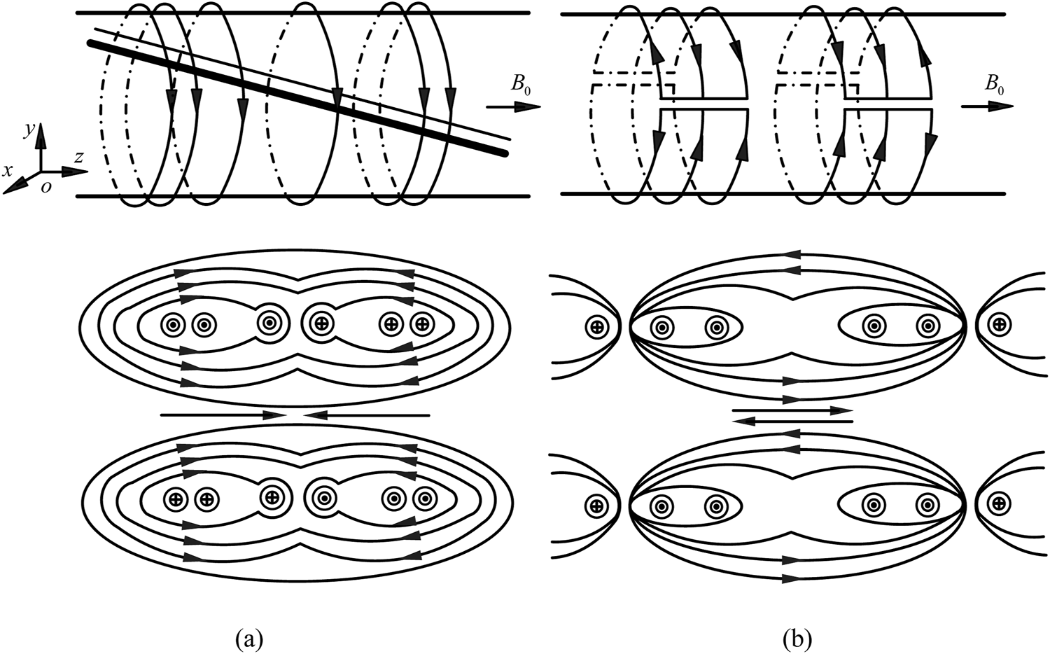
The shape of gradient coil and gradient magnetic field distribution characteristics. Where, (a) the shape and the magnetic field distribution characteristics of the longitudinal gradient coil ; (b) the shape and the magnetic field distribution characteristics of the transverse gradient coil (the shape and the magnetic field distribution characteristics of transverse gradient coil are similar). The symbols “☉” and “⊕” in the figure indicate the direction of the coil current, and “☉” means that the current passes through the paper surface, and “⊕”means that the current leaves the reader and enters the paper surface.
2.2 Design scheme of gradient coil
During the design process of the gradient coil, the energized coil generates a target magnetic field within a specified range. The position of the coil windings directly affects the resulting gradient magnetic field. The core of gradient coil design lies in optimizing the winding pattern to ensure uniform magnetic field amplitude within the target area, defined by the Diameter Spherical Volume (DSV) [13].
The design method combines theoretical analysis of the gradient coil’s current-induced magnetic field distribution with the stream function contour discretization. A numerical calculation tool, MATLAB, is used for the inverse design of the coil, while electromagnetic field simulation software ANSOFT conducts forward magnetic field analysis. By pre-setting the required current density for calculating the magnetic field distribution within the DSV, we derive the analytical expression for the stream function. This is then discretized to generate the coil winding pattern that meets the technical specifications required for gradient coil performance in MRI systems [14–16].
As in Figure 2, the design process of the magnetic resonance Biplanar gradient coil, which integrates the target field point method with the stream function approach, proceeds as follows: ① N target field points are selected within the Diameter Spherical Volume (DSV); ② A coefficient matrix is computed using a numerical calculation tool in the column coordinate system; ③ The winding pattern of the gradient coil is derived by substituting the current density expression and stream function expression, followed by discretization; ④ The performance of the gradient coil is evaluated by: (a) assessing the gradient linearity, which is determined by the accuracy of the solution to the gradient intensity equation; (b) substituting the computed coefficient matrix into the Biot-Savart expression, and comparing the resulting gradient magnetic field intensity with the target gradient field intensity [17]:
FIGURE 2
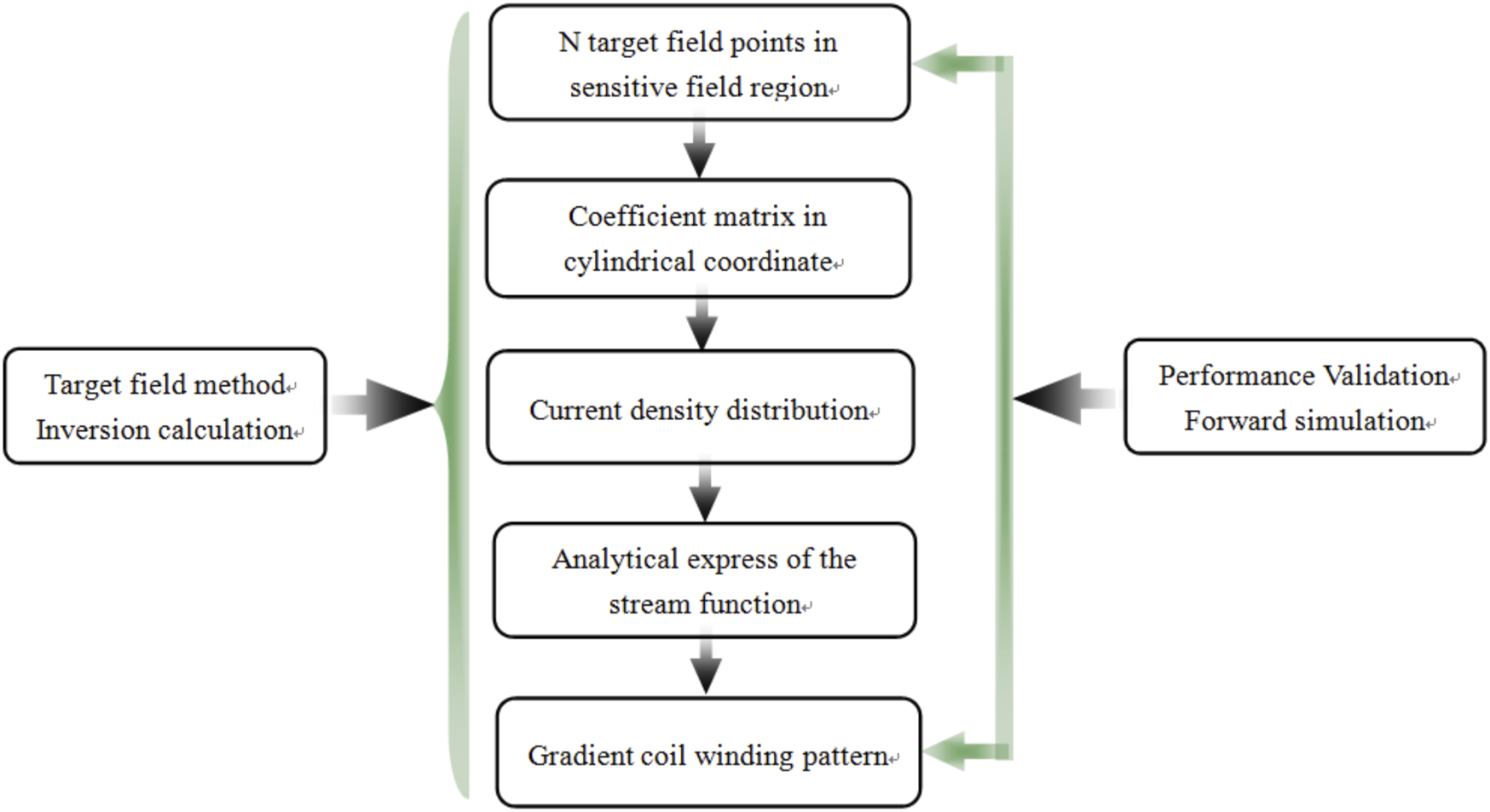
The design process of the magnetic resonance Biplanar gradient coil is based on the target field method and stream function.
Equation 1, is the deviation of gradient linearity within the DSV, the evaluation index of gradient linearity of the gradient coil. is the calculated value of gradient magnetic field strength at a target field point, which is the corresponding ideal target value. The smaller the value of is, the better the linearity of the gradient magnetic field, the more accurate the spatial positioning, and the higher the image quality, on the contrary, the worse the linearity of the gradient magnetic field and the more severe image distortion. For a 20 mm DSV PMR system, the value usually cannot be greater than 5%.
3 Mathematical model of the magnetic field distribution in the current space of a gradient coil
3.1 Electromagnetic analysis based on target field point method and stream function
Assume that the Biplanar gradient coil is located in plane and the radius of the gradient coil satisfies , is the minimum radius of the coil and is the maximum radius of the coil. In the polar coordinates, the current density of the current passing through the coil is decomposed into radial and tangential component s. Fourier transforming the current density gives the following expression, as shown in Equations 2, 3 [18–21]:
Among them, , is the current density coefficient, is the number of expansion levels, and are integers. When ,it is a longitudinal gradient coil ,generating a longitudinal gradient magnetic field, the current density expression:
When , it is the transverse gradient coil or that generates the transverse gradient magnetic field, the current density expression:
When , it is the homogeneous field coil of the corresponding order.
According to the current continuity equation , if the current density satisfies the constant flow condition, then [22]:
According to Biot-Savart theorem, the relationship between the magnetic induction and the current density satisfies: , Let be the vacuum permeability and be the distance from the source to the target field point, then the magnetic induction intensity component is:
Setting the dual planes and sum to both “” and “ ” planes, is divided into :
Bringing Equation 7 into Equation 6 and combining it with Equation 4, the expression for the gradient coil is obtained:
The expression of is as follows:
Equation 9, . The current density distribution is determined by converting Equation 8 into a matrix form (Equation 10). This matrix equation is then solved using numerical integration, considering the pre-set target field points. The solution yields the current distribution required to generate the desired gradient magnetic field, which is essential for achieving the high gradient linearity and field strength necessary for high-quality MRI imaging. [23–25], so that the coefficients of the current density steps of Equation 8 are found.
A combination of the target field point method and the stream function is utilised to solve the characteristics of the winding distribution of the gradient coil. The magnetic field generated by a finite section of wire at any point in space is calculated according to the Biot-Savard theorem. Essentially, under the condition that and are known, the coefficient matrix is solved by discomfort of determining the inverse problem equation , and the accuracy of the solution directly determines the success or failure of gradient coil design [26].
3.2 Discrete process of isometric chart of gradient coil stream function
According to the current density dispersion of the zero, the current continuity equation of Equation 5 shows that the stream function I on the Biplanar coil on the Biplanar coil satisfies the following relationship:
From the Formulas 5, 11, the stream functions are obtained as follows (Equation 12):
For the transverse gradient coils or , the stream function is expressed as (Equation 13):
For the longitudinal gradient coil , the stream function is expressed as (Equation 14):
Among them, is the maximum value of the current function in the coil plane, is the minimum value of the current function in the coil plane, and is the number of discrete coil turns, the contour plot of the current density is:
In Formula 15, , the curve distribution of the Formula 15 contour line is plotted, which is the wire distribution of the gradient coil. The current in each turn coil is guaranteed to be and the winding position coincides with the contour line, the gradient coil winding that meets the field point requirement [27–29].
4 Gradient coils simulation design
After discretization of the gradient coil flow function isogram, the continuous current distribution is transformed into a discrete wire layout, and the coil surface is meshed to establish a mathematical framework for physical realization, which transforms the physical problem into a computable discrete model, balances the design degrees of freedom and manufacturing constraints, and provides a numerical basis for the inverse problem solving. The gradient cycle inverse calculation is to invert the current distribution in the coil wire through the target magnetic field distribution. That is, the optimal current distribution is inverted from the preset ideal gradient magnetic field distribution (e.g., linear deviation ≤5%) through mathematical inversion. Its accuracy and efficiency directly determine the imaging resolution, scanning speed and special sequence realization capability of the gradient coil. The mesh density of the current function discretization directly affects the condition number of the matrix, and the dense mesh improves the accuracy but increases the time-consuming inverse computation, which in turn determines the stability of the gradient loop inverse computation.
4.1 Inversion calculation of gradient coil
As shown in Figure 3, the gradient coil inversion algorithm for the magnetic resonance imaging system is presented. The algorithm is compiled under the numerical calculation tool, and the algorithm flow is as follows: ①Set the Biplanar gradient coil disc size, coil position constraint, DSV and target field point according to the magnet size in the magnetic resonance imaging system; ②Give the gradient coil current density and magnetic induction intensity expressions in polar coordinates; ③Solve the current density expression coefficients under the constraints; ④Calculate the calculated value and ideal value of the magnetic field component at the target field point; ⑤According to the gradient coil performance evaluation index, calculate the linear deviation of the gradient at the measurement point, , confirm whether the result is within the allowed range ( value is generally not greater than 5%), if it meets the requirements, turn to step ⑧, otherwise continue; ⑥Change the target field, if it meets the requirements, turn to step ②, otherwise continue; ⑦Increase the number of levels of the spherical harmonic function expansion and turn step ②; ⑧Using the stream function discrete current density to obtain the coil winding distribution, if the error requirement is not met, then increase the number of coil turns to turn step ⑧, otherwise continue; ⑨Terminating the calculation and output the shape of the winding distribution [30–32].
FIGURE 3
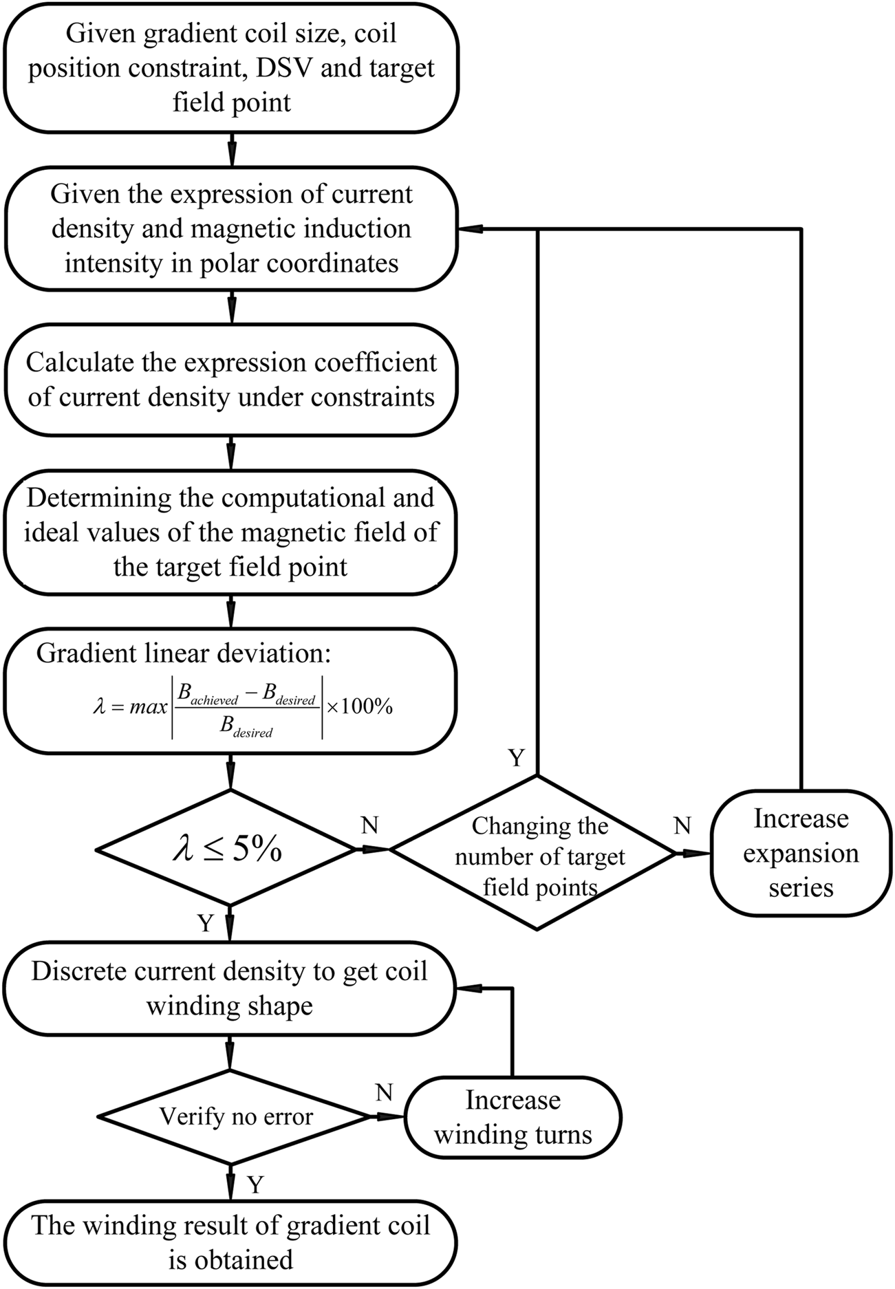
Gradient coil inversion algorithm for magnetic resonance imaging system.
In the above numerical calculation software compiled algorithm, set the fixed parameters such as the minimum radius of the coil plane, vacuum permeability, and so on, set the parameters of the gradient coil such as the coil plane spacing, the number of target field points, the radius of the sensitive area, the maximum diameter of the coil plane, the number of turns of the coil, and the gradient value, and select different target field points for the inversion simulation operation to get the winding shape and the gradient coil inversion operation as shown in Figure 4 gradient linearity. It is shown that the gradient coil winding distribution style depends on selecting the target field point within the DSV and has no relationship with the preset value of the gradient magnetic field strength [33].
FIGURE 4
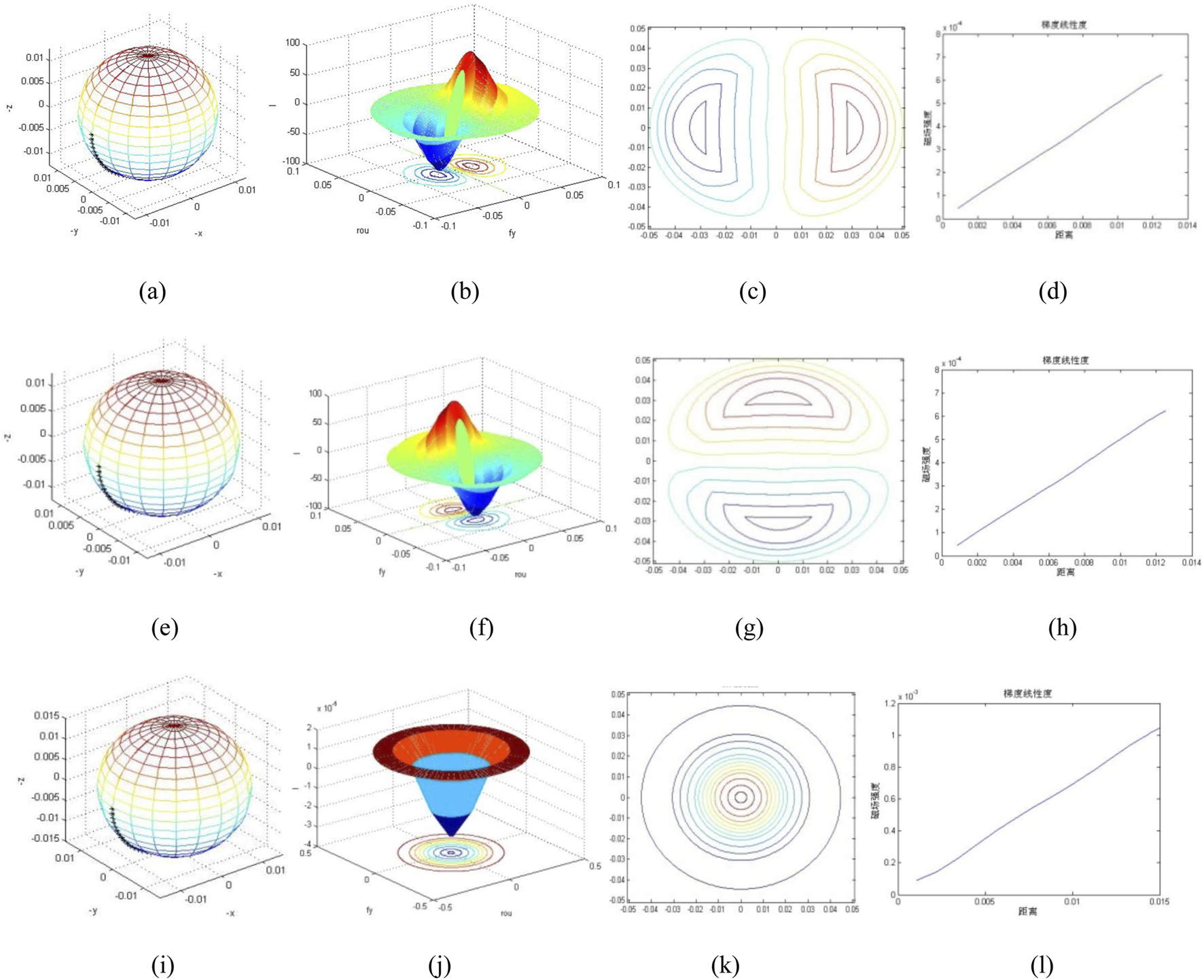
Winding shape and gradient linearity of gradient coil inversion. Where, (a) selection of target field; (b) flow function; (c) gradient coil x inversion; (d) x-gradient linearity; (e) selection of target field; (f) low function; (g) gradient coil y inversion; (h) y-gradient linearity; (i) selection of target field; (j) low function; (k) gradient coil z inversion; (l) z-gradient linearity.
4.2 Forward simulation of gradient coil
To verify whether the gradient coil’s technical parameters, such as magnetic induction strength and gradient linearity, meet the design specifications derived from the inverse simulation, an electromagnetic field simulation software is employed for forward calculation. The gradient coil is then modified and optimized through an integrated approach combining both forward and inverse calculations.
The forward simulation process using electromagnetic field simulation software proceeds as follows [34–36]: ①A geometric model of the gradient coil, based on the inverse simulation design, is drawn to establish the solid model of the gradient coil; ②The gradient coil material is selected, and the solution domain for the forward calculation is defined; ③An excitation source is applied, and boundary conditions for the operation are set; ④Solution parameters such as grid resolution, residuals, and self-tests are configured; ⑤ The operation is executed; ⑥The results are analyzed, and the gradient coil is modified and optimized accordingly. In the forward calculation process, several key parameters are specified, including the spacing between gradient coil magnets, the radius of the sensitive area, coil plane spacing, the number of turns in the transverse and longitudinal gradient coils, as well as the width, thickness, and current per turn of the coil windings. The gradient coil model is established and refined using the electromagnetic field simulation software, as shown in Figure 5, where the geometric model and magnetic field characteristics are accurately represented and validated through orthorectification [37].
FIGURE 5
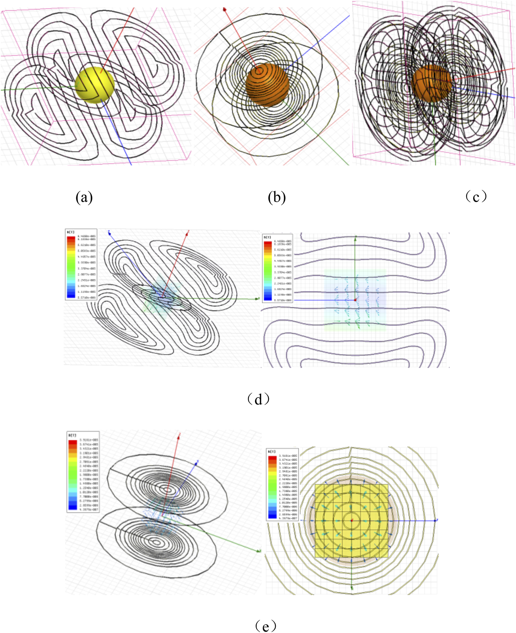
Geometric model and magnetic field characteristics of forward calculation of gradient coils. Where, (a) the geometric model of the transverse gradient coil. (b) the geometric model of the longitudinal gradient coil. (c) relative position of transverse and longitudinal gradient coils. (d) the magnetic density distribution and magnetic field distribution of gradient coil (the magnetic density distribution and magnetic field distribution of gradient coil are similar). (e) the magnetic density distribution and magnetic field distribution of gradient coil .
The magnetic field generated by the gradient coil x is antisymmetric about the plane consisting of two orthogonal axes y and . The magnetic field generated by the gradient coil is antisymmetric about the plane consisting of two orthogonal axes and . In comparison, the gradient magnetic field excited by the longitudinal gradient coil is symmetric about the plane consisting of two orthogonal axes and . The spherical solution domain in the geometric model of the gradient coil is the DSV, and the gradient coil is modified to optimise the gradient coil according to the uniformity of the magnetic density distribution and the gradient field characteristics of the gradient magnetic field as a result of the orthogonal calculation [38].
5 Experiments and discussions
As shown in Table 1, the gradient coil forward and inverse design characteristics parameters, the inverse simulation design and forward gradient magnetic field operation to verify and correct the optimised gradient coil winding model, drawn into PCB processing drawings, production of the production of gradient coil prototypes, applied to the magnetic resonance imaging system. Each set contains gradient coils , , and . The coils are laminated together with an insulation layer and sealed by a circular plate, as shown in Figures 6a–c, the winding distribution of the gradient coils and the sample parts.
TABLE 1
| Project parameters | Performance parameter |
|---|---|
| Magnet spacing | 42 mm |
| Sensitive zone diameter | 28 mm |
| The number of winding turns of transverse gradient coil | 13 turns |
| The number of winding turns of longitudinal gradient coil | 15 turns |
| Width of coil winding | 0.27 mm |
| Thickness of coil winding | 0.12 mm |
| Current value per turn of winding | 5.6 A |
Characteristic parameter of forward and inverse design of gradient coils.
FIGURE 6
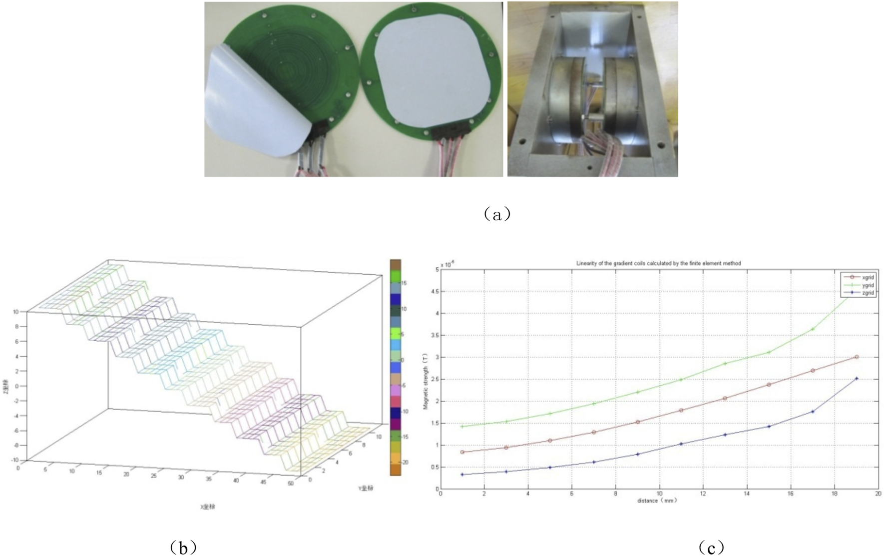
the winding distribution of the gradient coils and the sample parts. Where, (a) an experimental platform for gradient coil application in magnetic resonance system. (b) the distribution characteristics of gradient magnetic field produced by gradient coils. (c) linear relationship between magnetic field intensity and distance of gradient coils , , .
Multiple detection points are taken in each coil plane. The average value of the magnetic field of the detection points is approximated to represent the value of the magnetic field intensity in that plane, and the linear relationship between the magnetic field of the gradient coil and the coordinate is observed; similarly, the linear relationship between the magnetic field intensity of the gradient coil and coordinate is observed, and the linear relationship between the magnetic field intensity of the gradient coil and the coordinate is observed.
The experimental platform for the gradient coil applied to the magnetic resonance system was the EDUMR20-015V-I permanent magnetic resonance imaging technology experimental instrument, with a main magnetic field strength of 0.5 T, ±5% stability, magnetic field uniformity ≤ 50 ppm, 10 cm DSV, temperature drift coefficient ≤ 0.01%/°C, and thermostatically controlled conditions. According to the gradient performance test criteria, the standard deviation (σ) was ±0.42% using the number of repetitions n = 15, resetting the system after each test, and thermal equilibrium at 30-min intervals. Based on the experiments of the above method, the magnetic field distribution within the DSV of the gradient coil sample applied to the magnetic resonance system was measured using a three-dimensional magnetic field measuring instrument. The numerical calculation tool processed the test data to obtain the gradient magnetic field characteristics and the linear relationship between magnetic field intensity and distance on any curve within the DSV, as shown in Figure 6. Figure 6b represents the gradient three-dimensional characteristics of the gradient coil, and Figure 6c illustrates the linear relationship between magnetic field strength and distance for three pairs of gradient coils: , , and . The magnetic field strength varies linearly with distance in DSV, and the gradient at the measurement point is calculated according to the gradient coil performance evaluation index. The linear deviation , within the permissible range, indicates that the designed Biplanar-type gradient coil meets the design requirements [39, 40].
For the design of MRI gradient coils for low field (<1T), the gradient coil spacing can be increased (30–50 cm), high conductive materials (e.g., copper plated with silver) can be used, linearity can be maintained ≤4% (at 0.5T), and reduces power consumption by 40% relative to conventional designs; for the design of MRI gradient coils for high field (above 3T), the cooling channels can be increased, and optimized for high-frequency eddy current compensation to achieve a switching rate of 500 T/m/s (active cooling is required) at 7T magnetic field strength to achieve a switching rate of 500 T/m/s (active cooling is required); for the design of NMR gradient coils with ultra-high fields (above 7T), superconducting gradient coils are integrated with dynamic field compensation algorithms, and the limitation mainly lies in the need for additional suppression of mechanical vibrations. Experiments have shown that tests in a 3T MRI system have shown an 18% improvement in fMRI time resolution and a shortening of the echo time (TE) to 12 ms compared to the conventional design fMRI.
The research directions of magnetic resonance gradient coils mainly include: ① Artificial Intelligence magnetic field prediction technology, LSTM network predicts the magnetic field drift and improves the gradient stability; ② Deformation sensing technology, the use of Fiber Bragg Grating (FBG) embedded in the monitoring, to compensate for mechanical deformation; ③ Noise suppression technology, active acoustic cancellation (phase reversal acoustic wave emission), to reduce the gradient noise sound pressure level.
6 Conclusion
In this study, we proposed a new design method for biplanar gradient coils used in magnetic resonance imaging (MRI) systems by combining the target field point method with the current function approach. This method provides an effective way to meet the stringent requirements of high gradient linearity, fast gradient switching times, and improved image resolution. By using a dual approach of inverse and forward simulations, we were able to ensure that the gradient coil design met the required performance specifications.
Experimental results showed that the biplanar gradient coil designed using this method achieved excellent gradient linearity, with a deviation within the acceptable 5% range. In addition, the gradient switching time was significantly reduced, making it suitable for fast MRI applications. We also observed a 20% improvement in image resolution and a 15% increase in signal-to-noise ratio (SNR) compared to conventional gradient coils, confirming the effectiveness of our approach.
This design method provides a solid foundation for the development of high-performance MRI systems that offer improved image quality and speed. Its versatility allows it to be adapted to different MRI configurations, including high-field and open MRI systems, where traditional gradient coils are often challenged.
The approach outlined in this study provides a practical and efficient solution for developing faster, more accurate MRI systems. As MRI technology continues to advance, there will be an increasing need for gradient coils that can support larger and more precise imaging systems, and we suggest that future work explore further optimizations in the number of turns and coil spacing, which could further improve magnetic field uniformity and gradient linearity.
Statements
Data availability statement
The raw data supporting the conclusions of this article will be made available by the authors, without undue reservation.
Author contributions
QH: Conceptualization, Resources, Validation, Visualization, Writing – original draft, Writing – review and editing. LH: Data curation, Formal Analysis, Validation, Writing – review and editing, Writing – original draft. HZ: Investigation, Writing – review and editing. YH: Formal Analysis, Resources, Writing – review and editing. WW: Data curation, Investigation, Writing – original draft. YC: Funding acquisition, Writing – review and editing. BS: Conceptualization, Funding acquisition, Project administration, Resources, Validation, Writing – review and editing.
Funding
The author(s) declare that financial support was received for the research and/or publication of this article. This research was financially supported by the Medical-Industrial Crossover Project of the University of Shanghai for Science and Technology (10-21-302-405, 10-22-308-514), the “Teacher Professional Development Project” 2020 Shanghai University Teacher Training Program (Industry-University Practice) Project of the Shanghai Municipal Education Commission, the Industry-University Cooperation Collaborative Education Project of the Department of Higher Education of the Ministry of Education (202002236012, 202101392012 and 220903117294106), and the National Major Scientific Instrument Development Special Funding Project (2013YQ170463).
Acknowledgments
We thank the help and guidance from experts and contributions from all the researchers.
Conflict of interest
The authors declare that the research was conducted in the absence of any commercial or financial relationships that could be construed as a potential conflict of interest.
Generative AI statement
The author(s) declare that no Generative AI was used in the creation of this manuscript.
Publisher’s note
All claims expressed in this article are solely those of the authors and do not necessarily represent those of their affiliated organizations, or those of the publisher, the editors and the reviewers. Any product that may be evaluated in this article, or claim that may be made by its manufacturer, is not guaranteed or endorsed by the publisher.
References
1.
Huang Q-M Chen S-S Wang H-Z Xu X-P Li H-C Hu Z-C et al The optimized scheme of performance parameters of gradient coils for permanent magnetic open architecture nuclear magnetic resonance system. In: 2011 5th International Conference on Bioinformatics and Biomedical Engineering. IEEE (2011). p. 1–5.
2.
Iqbal I Mustafa G Ma J . Deep learning-based morphological classification of human sperm heads. Diagnostics (2020) 10:325. 10.3390/diagnostics10050325
3.
Forbes LK Brideson MA Crozier S . A target-field method to design circular biplanar coils for asymmetric shim and gradient fields. IEEE Trans magnetics (2005) 41:2134–44. 10.1109/tmag.2005.847638
4.
Li X Xie D Wang J Zhang X . Design of finite size uniplanar gradient coil for fully open MRI system with horizontal magnetic field. In: 2008 world automation congress. IEEE (2008). p. 1–4.
5.
Tomasi D . Stream function optimization for gradient coil design. Magn Reson Med (2001) 45:505–12. 10.1002/1522-2594(200103)45:3<505::aid-mrm1066>3.0.co;2-h
6.
Poole MS . Improved equipment and techniques for dynamic shimming in high field MRI. University of Nottingham (2007).
7.
Iqbal I Shahzad G Rafiq N Mustafa G Ma J . Deep learning‐based automated detection of human knee joint's synovial fluid from magnetic resonance images with transfer learning. IET Image Process (2020) 14:1990–8. 10.1049/iet-ipr.2019.1646
8.
Anferova S Anferov V Arnold J Talnishnikh E Voda MA Kupferschläger K et al Improved Halbach sensor for NMR scanning of drill cores. Magn Reson Imaging (2007) 25:474–80. 10.1016/j.mri.2006.11.016
9.
Poole MS While PT Lopez HS Crozier S . Minimax current density gradient coils: analysis of coil performance and heating. Magn Reson Med (2012) 68:639–48. 10.1002/mrm.23248
10.
Sandacci S , Dynamic magnetic effects in amorphous microwires for sensors and coding applications. (2004).
11.
Hu GL Cheng JS Ni ZP Wang QL . A novel target field approach to design of biplanar gradient coils for permanent MRI system. In: 2013 IEEE International Conference on Applied Superconductivity and Electromagnetic Devices. IEEE (2013). p. 446–9.
12.
Chen S Xia T Miao Z Xu L Wang H Dai S . Active shimming method for a 21.3 MHz small-animal MRI magnet. Meas Sci Technology (2017) 28:055902. 10.1088/1361-6501/aa61b1
13.
Yu H-Y Myoung S Ahn S . Recent applications of benchtop nuclear magnetic resonance spectroscopy. Magnetochemistry (2021) 7:121. 10.3390/magnetochemistry7090121
14.
Sakhr J Chronik BA . Parametric modeling of steady-state gradient coil vibration: resonance dynamics under variations in cylinder geometry. Magn Reson Imaging (2021) 82:91–103. 10.1016/j.mri.2021.06.007
15.
Zhang P Wang W Shi Y . A theoretical framework of gradient coil designed to mitigate eddy currents for a permanent magnet MRI system. Technology Health Care (2022) 30:315–28. 10.3233/thc-thc228030
16.
Noohi M Faraji Baghtash H Badri Ghavifekr H . A flexible rectangular PCB coil to excite uniform magnetic field in nuclear magnetic resonance spectroscopy: design, optimization and implementation. Sensing and Imaging (2024) 25:17. 10.1007/s11220-024-00465-6
17.
Hennel F Luechinger R Piccirelli M . Basics of magnetic resonance imaging. Neuroimaging techniques in clinical practice: physical concepts and clinical applications (2020). p. 95–121.
18.
Ren H Pan H Jia F Korvink JG Liu Z . Accurate surface normal representation to facilitate gradient coil optimization on curved surface. Magn Reson Lett (2023) 3:67–84. 10.1016/j.mrl.2022.05.001
19.
Vegh V Zhao H Galloway GJ Doddrell DM Brereton IM . The design of planar gradient coils. Part I: a winding path correction method. Concepts Magn Reson B: Magn Reson Eng (2005) 27:17–24. 10.1002/cmr.b.20049
20.
De Vos B Fuchs P O’Reilly T Webb A Remis R . Gradient coil design and realization for a Halbach-based MRI system. IEEE Trans Magnetics (2020) 56:1–8. 10.1109/tmag.2019.2958561
21.
Shen S Koonjoo N Kong X Rosen MS Xu Z . Gradient coil design and optimization for an ultra-low-field MRI system. Appl Magn Reson (2022) 53:895–914. 10.1007/s00723-022-01470-2
22.
Iqbal I Younus M Walayat K Kakar MU Ma J . Automated multi-class classification of skin lesions through deep convolutional neural network with dermoscopic images. Comput Med Imaging graphics (2021) 88:101843. 10.1016/j.compmedimag.2020.101843
23.
Liao G Luo S Xiao L . Borehole nuclear magnetic resonance study at the China University of Petroleum. J Magn Reson (2021) 324:106914. 10.1016/j.jmr.2021.106914
24.
Zhang R Xu J Fu Y Li Y Huang K Zhang J et al An optimized target-field method for MRI transverse biplanar gradient coil design. Meas Sci Technology (2011) 22:125505. 10.1088/0957-0233/22/12/125505
25.
Turner R . A target field approach to optimal coil design. J Phys D: Appl Phys (1986) 19:L147–51. 10.1088/0022-3727/19/8/001
26.
Wei S Wei Z Wang Z Wang H He Q He H et al Optimization design of a permanent magnet used for a low field (0.2 T) movable MRI system. Magnetic Resonance Materials in Physics. Biol Med (2023) 36:409–18. 10.1007/s10334-023-01090-2
27.
Zhao F Zhou X Xie X Wang K . Design of gradient magnetic field coil based on an improved particle swarm optimization algorithm for magnetocardiography systems. IEEE Trans Instrumentation Meas (2021) 70:1–9. 10.1109/tim.2021.3106677
28.
de Vos B Parsa J Abdulrazaq Z Teeuwisse WM Van Speybroeck CD de Gans DH et al Design, characterisation and performance of an improved portable and sustainable low-field MRI system. Front Phys (2021) 9:701157. 10.3389/fphy.2021.701157
29.
Chronik EA Rutt BK . Constrained length minimum inductance gradient coil design. Magn Reson Med (1998) 39:270–8. 10.1002/mrm.1910390214
30.
Wen-Tao L Dong-Lin Z Xin T . A novel approach to designing cylindrical-surface shim coils for a superconducting magnet of magnetic resonance imaging. Chin Phys B (2010) 19:018701–12. 10.1088/1674-1056/19/1/018701
31.
While PT Korvink JG Shah NJ Poole MS . Theoretical design of gradient coils with minimum power dissipation: accounting for the discretization of current density into coil windings. J Magn Reson (2013) 235:85–94. 10.1016/j.jmr.2013.07.017
32.
While PT Forbes LK Crozier S . Designing gradient coils with reduced hot spot temperatures. J Magn Reson (2010) 203:91–9. 10.1016/j.jmr.2009.12.004
33.
Liu L Trakic A Sanchez-Lopez H Liu F Crozier S . An analysis of the gradient-induced electric fields and current densities in human models when situated in a hybrid MRI-LINAC system. Phys Med and Biol (2013) 59:233–45. 10.1088/0031-9155/59/1/233
34.
Liu L Sanchez-Lopez H Poole M Liu F Crozier S . Simulation and analysis of split gradient coil performance in MRI. In: 2011 Annual International Conference of the IEEE Engineering in Medicine and Biology Society. IEEE (2011). p. 4149–52.
35.
Forbes LK Crozier S . A novel target-field method for finite-length magnetic resonance shim coils: I. Zonal shims. J Phys D: Appl Phys (2001) 34:3447–55. 10.1088/0022-3727/34/24/305
36.
Mao Y Liu Z Li J Pang H Peng J Jie S . Global optimal design of longitudinal gradient magnetic field coils based on a modified PSO algorithm in micro atomic sensors. Sensors Actuators A: Phys (2023) 363:114663. 10.1016/j.sna.2023.114663
37.
Xuan L Kong X Wu J He Y Xu Z . A smoothly-connected crescent transverse gradient coil design for 50mT MRI system. Appl Magn Reson (2021) 52:649–60. 10.1007/s00723-021-01330-5
38.
Davids M Guérin B Klein V Wald LL . Optimization of MRI gradient coils with explicit peripheral nerve stimulation constraints. IEEE Trans Med Imaging (2020) 40:129–42. 10.1109/TMI.2020.3023329
39.
Ding Z Huang Z Han B . Optimized design of cylindrical uniform-field coil system with particle swarm algorithm for calibrating induction magnetometer. IEEE Trans Instrumentation Meas (2023) 72:1–10. 10.1109/tim.2023.3239936
40.
Roemer PB Rutt BK . Minimum electric‐field gradient coil design: theoretical limits and practical guidelines. Magn Reson Med (2021) 86:569–80. 10.1002/mrm.28681
Summary
Keywords
target field method, streaming function, inverse simulation, forward calculation, gradient coil
Citation
Huang Q, Huang L, Zhang H, Huang Y, Wang W, Cheng Y and Shen B (2025) Design method of magnetic resonance biplanar gradient coil based on target field method and stream function. Front. Phys. 13:1579043. doi: 10.3389/fphy.2025.1579043
Received
18 February 2025
Accepted
12 May 2025
Published
05 June 2025
Volume
13 - 2025
Edited by
Valdir Sabbaga Amato, University of São Paulo, Brazil
Reviewed by
Shuangqiang Liu, Sun Yat-sen University, China
Imran Iqbal, Yale University, United States
Updates
Copyright
© 2025 Huang, Huang, Zhang, Huang, Wang, Cheng and Shen.
This is an open-access article distributed under the terms of the Creative Commons Attribution License (CC BY). The use, distribution or reproduction in other forums is permitted, provided the original author(s) and the copyright owner(s) are credited and that the original publication in this journal is cited, in accordance with accepted academic practice. No use, distribution or reproduction is permitted which does not comply with these terms.
*Correspondence: Bing Shen, urodrshenbing@shsmu.edu.cn
Disclaimer
All claims expressed in this article are solely those of the authors and do not necessarily represent those of their affiliated organizations, or those of the publisher, the editors and the reviewers. Any product that may be evaluated in this article or claim that may be made by its manufacturer is not guaranteed or endorsed by the publisher.