

 Casimir J. H. Ludwig and Iain D. Gilchrist
- School of Experimental Psychology, University of Bristol, Bristol, UK
A growing number of studies in vision research employ analyses of how perturbations in visual stimuli influence behavior on single trials. Recently, we have developed a method along such lines to assess the time course over which object velocity information is extracted on a trial-by-trial basis in order to produce an accurate intercepting saccade to a moving target. Here, we present a simplified version of this methodology, and use it to investigate how changes in stimulus contrast affect the temporal velocity integration window used when generating saccades to moving targets. Observers generated saccades to one of two moving targets which were presented at high (80%) or low (7.5%) contrast. In 50% of trials, target velocity stepped up or down after a variable interval after the saccadic go signal. The extent to which the saccade endpoint can be accounted for as a weighted combination of the pre- or post-step velocities allows for identification of the temporal velocity integration window. Our results show that the temporal integration window takes longer to peak in the low when compared to high contrast condition. By enabling the assessment of how information such as changes in velocity can be used in the programming of a saccadic eye movement on single trials, this study describes and tests a novel methodology with which to look at the internal processing mechanisms that transform sensory visual inputs into oculomotor outputs.
Introduction
Saccadic eye movements serve to orient the fovea onto an object or region of interest within the visual environment. These movements are the result of a decision process that is typically based on the analysis of sensory information, and so offer an ideal route through which to assess how decision-making mechanisms may be implemented by sensorimotor circuits in the brain (Gold and Shadlen, 2001, 2007; Glimcher, 2001; Schall, 2003). In recent years, there has been growing interest in the development of methods with which to assess how perceptual signals inform eye movement decisions (Beutter et al., 2003; de Brouwer et al., 2002; Caspi et al., 2004; Ludwig et al., 2005, 2007; Bennett et al., 2007; Eckstein et al., 2007; Spering et al., 2007; Nummela et al., 2008; Tavassoli and Ringach, 2009; Etchells et al., 2010).
Although the questions under investigation in these various studies differed, as did the precise methods used, there is a common theme. In general, a visual stimulus is perturbed in some way or another (e.g., adding random luminance noise over time in Caspi et al., 2004 and Ludwig et al., 2005). Careful analysis of how this perturbation influences behavior on single trials then enables estimation of the spatial and/or temporal portions of the stimulus that preferentially drive decisions, through a variety of techniques (e.g., reverse correlation or logistic regression approaches). Important new insights have been obtained with these methodologies. For instance, Caspi et al. (2004) were able to show that the uptake of visual information in a single fixation drove not only the immediately following eye movement decision, but also the one after that. Ludwig et al. (2005) showed that decisions were driven by visual information time-locked to display onset, rather than saccade onset. Indeed, these authors showed that only a remarkably short portion of the overall latency period was used to integrate the sensory evidence (see also Ludwig, 2009).
Recently, we have developed a related method to assess over what time interval object velocity information is extracted in order to accurately intercept a moving object with a saccade (Etchells et al., 2010). Targeting a moving object poses a challenging decision problem: sensory input and motor output delays, as well as the eye movement duration itself, will result in a delay between the decision being made to generate an eye movement and the actual completion of that movement (Kerzel and Gegenfurtner, 2003). Consequently, some decision has to be made regarding how far ahead of the “currently seen” object position a saccade is to land, given the continued object motion during movement programming and execution. Clearly, having an estimate of the object velocity is desirable for this purpose.
Our method to identify the epoch over which this information is extracted, follows the same logic as presented above (and is closely related to the double-step method used to infer over what epoch position information is extracted; Becker and Jürgens, 1979). Observers are presented with two targets moving at a particular velocity. A “go” signal indicates which object observers have to saccade to. At some point after the go signal, target velocity is perturbed: the objects abruptly speed up or slow down. The random variation from trial-to-trial in the timing of the speed step, coupled with the natural variability in saccade latency, can be used to build up a picture of how much time the saccadic system needs to be able to incorporate information about the second speed into the saccade program.
The landing position on each trial may be used to estimate the relative weights attributed to the pre- and post-step velocities, by comparing the observed endpoint with the predicted endpoints based on the two velocities. We then assess how these weights change as a function of time from saccade onset. For instance, if the velocity step occurs long before movement onset the observer will have had more time to base their decision on the post-step, veridical velocity. As will be explained in detail below, fitting these weights over time with a model provides an estimate of the time interval over which object velocity was extracted.
Our previous work suggests that the system used a temporal window with a duration of ∼100 ms to estimate target velocity (Etchells, et al., 2010). The end of the window is positioned ∼80 ms before the onset of the saccade. The latter period may be considered the saccadic dead-time, which is functionally defined as the period during which new visual information can no longer affect the saccade endpoint (Becker and Jürgens, 1979; Findlay and Harris, 1984; Aslin and Shea, 1987; Ludwig et al., 2007). The observed endpoint from each trial is converted into a relative weight associated with the post-step velocity. These weights are then fitted with some functional form.
Our model is not a process model that specifies the visual mechanisms involved in velocity estimation. However, there is a process interpretation of the model, which is illustrated in Figure 1. We assume that during the latency period object velocity is estimated by convolving the input velocities with some temporal filter (Benton and Curran, 2009) such as that seen in Figure 1. This operation is analogous to computing a running, weighted average of the input. The temporal integration performed by the filter necessarily results in a certain amount of blurring of the velocity information when the velocity is variable. As a result, the observed endpoints may not simply reflect either the pre-step velocity or the post-step velocity, but may be driven by intermediate velocity estimates. The prediction period shown in the figure is assumed to consist of the dead-time and the saccade duration itself.
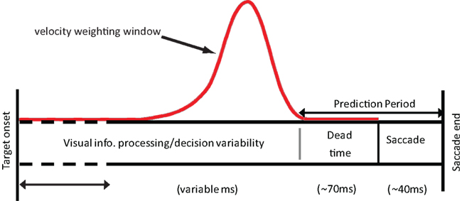
Figure 1. The time course of a saccade from target detection to the end of the saccade. During this time, average velocity is estimated using a weighting window similar in nature to the one shown here (red solid line). The target is assumed to move at this averaged velocity during the prediction period. This information can then be used to determine where the target is likely to be located at the end of the saccade.
In the present study, our aims were twofold. First, we sought to validate this process interpretation of the model using a straightforward manipulation of the input which is known to profoundly affect the visual system: a variation in contrast. Second, we aimed to simplify the method of fitting the model to make it more user-friendly. The model presented by Etchells et al. (2010) included specification and estimation of a multitude of noise sources that, together, produced variability in the velocity weights (e.g., variability in saccade duration, which is correlated with variability in saccade amplitude). In this article we describe and test a significant simplification, which essentially combines all noise sources together and eases the estimation of the critical parameters of interest: those that describe the velocity weighting function.
In the model presented in Etchells et al. (2010), observers were presented with targets that did not differ in contrast from trial-to-trial. In the current study, in order to test and demonstrate our simplified model, we examine the effects of changing stimulus contrast on velocity integration. The work in the current paper therefore presents (1) a methodological advance in the form of a simple technique for characterizing the incorporation of velocity information into saccadic planning, and (2) an empirical advance in the form of a quantification of the effects of changing contrast on velocity integration during saccade planning. A wealth of research over the past 50 years has given us detailed knowledge of how contrast affects the visual system (e.g., Mansfield, 1973; Breitmeyer, 1975; Harwerth and Levy, 1978; Plainis and Murray, 2000; Weiss et al., 2002; Murray and Plainis, 2003; Carpenter, 2004; Ludwig et al., 2004; Taylor et al., 2006; White et al., 2006) and its underlying neurophysiology (e.g., Enroth-Cugell and Robson, 1966; Pack et al., 2005; Krekelberg et al., 2006; Livingstone and Conway, 2006). Consequently, we can make some informed predictions about the effect that contrast will have on the generation of saccades to moving targets.
Weiss et al. (2002) suggest that at low-contrast, there is less precise information about the actual speed of a given stimulus. The greater level of uncertainty is represented by an increase in the spread of the likelihood function of target velocity estimates. In other words, reducing stimulus contrast corresponds to a decrease in the signal-to-noise ratio (SNR) of the velocity measurement. If the velocity weighting function we measure with our method maps onto the underlying temporal filter used to estimate velocity, we might reasonably expect the width of the filter to increase when the target contrast is low. By extending the amount of time during which the velocity signal is sampled and averaged, SNR is increased to obtain a more precise estimate of target velocity.
Alternatively, a reduction in contrast may result in an increase in the time it takes for the incoming velocity information to reach the integration mechanism, as a result of increasing neuronal conduction latencies (e.g., Kaplan and Shapley, 1982). For example, Maunsell et al. (1999) showed that, depending on the number of inputs summed, latency differences in the magnocellular pathway through the lateral geniculate nucleus (LGN) are likely to be on the order of 5–15 ms between high and low intensity stimuli, with high intensity stimuli producing faster responses. A change in the velocity of the lower contrast stimulus will therefore take a longer time to register, which would result in a delay in the velocity signal reaching the integration mechanism. In our methodology, the time-to-peak of the velocity weighting function reflects the time at which emphasis is shifted onto more recent velocity inputs. Therefore, when contrast is reduced, we might expect to see a delay in the point at which a velocity change is detected and incorporated into the final velocity estimate.
Experimental Overview
Observers were required to fixate a central diamond-shaped fixation stimulus on a computer screen whilst two Gaussian patches (SD = 0.32°) traversed horizontally across the screen, 6° above and below the midline. During the trial, the fixation point would change into either an upwards- or downwards-pointing arrow, indicating which patch the observers had to make a saccade to (see Figure 2A). On some trials, after a variable delay the speed of the patches would change. By looking at the relationship between saccade landing positions and the time of the speed changes, we can determine how the saccadic system weighs the two velocities over time. We examine the nature of this velocity integration function in two conditions: high and low-contrast.
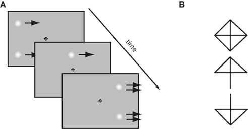
Figure 2. (A) Outline of the time course for a rightwards, step up trial. Gaussian patches start moving rightward. After some interval of time the fixation stimulus changes to an arrow, signaling that a saccade to the top patch should be made. After this, the patches step up in speed (illustrated by the double arrows). Note that patches and fixation point are not to scale, for illustration purposes. (B) The fixation stimulus. Removal of either the bottom two or top two diagonal line segments results in an arrow indicating which patch to saccade to.
Observers
Six observers were recruited from the students of the University of Bristol, UK (3 females, age range 24–30, mean age 26.0). All had self-reported normal or corrected-to-normal vision. Data were collected over the course of four sessions, performed on different days. The study was approved by the local ethics committee.
Eye Movement Recording
Stimuli were displayed on a 21-inch, gamma-corrected CRT monitor (LaCie Electron Blue) running at 75 Hz. The monitor resolution was 1152 × 864 pixels, and the screen subtended 36° × 24° of visual angle. An Eyelink 1000 system (SR Research, Mississauga, ON, Canada) was used to record and monitor eye movements. This is an infrared tracking system that uses the pupil center in conjunction with corneal reflection to sample eye position at 1000 Hz. For each data sample, a dedicated parser algorithm (SR Research, Mississauga, ON, Canada) computes the instantaneous velocity and acceleration of the eye. These are then compared to threshold criteria for velocity (30°/s) and acceleration (8000°/s2). If either is above threshold, the eye movement is classified as a saccade. Visual inspection of a random selection of saccades confirmed that the automatic algorithm placed the on and offsets of the saccades appropriately, without including any apparent contributions from the potential pursuit component that may have followed the saccade. Head position was stabilized at a viewing distance of 57 cm via the use of the Eyelink 1000 built-in chin rest. Observers viewed the display monocularly using their dominant eye, and eye dominance was measured using the hole-in-the-card technique (Seijas et al., 2007). The experimental software was programmed in MATLAB using the Psychophysics Toolbox (Brainard, 1997) and Eyelink Toolbox extensions (Cornelissen et al., 2002).
Design and Procedure
Observers performed 28 experimental blocks, each containing 128 trials. Prior to each block, a nine-point calibration procedure was performed in which observers were asked to fixate a black cross that appeared randomly on a 3 × 3 grid. The fixation stimulus measured 0.3° × 0.3°, and the calibration grid subtended 31° × 19° of visual angle. On a given trial, observers were instructed to fixate a central stimulus which took the form of a black diamond containing a cross (see Walker et al., 2000, Experiment 2). Observers were instructed which patch to make a saccade to by the removal of either the top two or bottom two diagonal segments, respectively forming either a downwards or upwards arrow (see Figure 2B).
In 50% of the trials within each block, the Gaussian patches would start moving at a constant speed of 18°/s and remain at this speed for the duration of the trial. In 25% of the trials, the patches would step up from 18 to 30°/s at a variable time after the change in fixation stimulus. In the remaining 25% of the trials, the patches would step down to 6°/s. The patches were shown for at least 445 ms before the change in fixation stimulus would occur. After this time, an exponential, i.e., “non-aging,” foreperiod (Nickerson and Burnham, 1969; Oswal et al., 2007) was used to determine the time of the fixation change. A non-aging foreperiod can be described as one in which the probability of a target appearing in the next time interval decreases exponentially over time. This results in an observer’s expectation remaining constant over the course of a trial, which avoids portions of the observer’s response being attributable to something other than the visual information in the stimulus. The mean of this exponential distribution was 128 ms. A second non-aging foreperiod, with a mean of 100 ms, was used to determine the time of the speed step. In both cases, a maximum cumulative probability of 95% was used to truncate the distribution, in order to prevent the generation of extremely long foreperiods that would take the patterns off the screen.
Within each block the contrast of the patches remained the same, with contrasts being randomized between blocks. Half of the blocks were presented at a high contrast and half at low-contrast. Contrast was defined as Lmax − Lo/Lo where Lo indicates background luminance. This gives contrast values of 80% in the high condition (Lmax = 65.4 cd/m2, Lo = 36.4 cd/m2) and 7.5% in the low condition (Lmax = 39.1 cd/m2, Lo = 36.4 cd/m2).
Data Analysis
Only data describing the first saccade in each trial were considered. As the minimum distance between the fixation point and target was 6° (when the target was located directly above or below fixation), trials in which the amplitude of the first saccade was less than 4° were rejected, as were trials in which no saccade was generated. Saccade endpoints were recorded, along with the target location at saccade termination and saccade amplitude. The primary analysis concerned the horizontal component of each saccade.
Results
For each contrast condition, we first want to determine the extent to which the first orienting saccade is influenced by the pre- and post-step velocities. We do this by measuring, for each trial, the horizontal error between where the saccade landed, and where the target was at the end of the saccade. This saccade endpoint error is then plotted as a function of the time between the velocity step and saccade onset, which we term D. This is aligned on saccade onset, such that D = 0 ms corresponds to the start of the saccade, and D = 500 ms corresponds to the velocity step occurring 500 ms before saccade onset.
Figure 3 shows, for a single observer, this landing position error as a function of D for both high and low-contrast conditions.
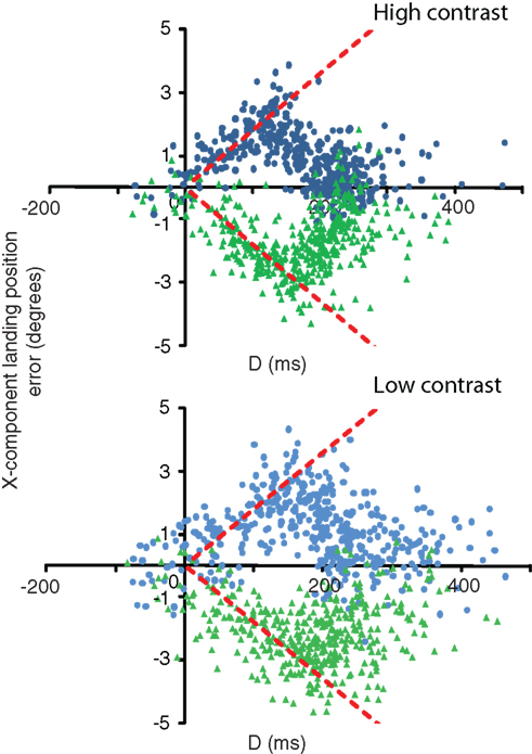
Figure 3. D (time between velocity change and saccade onset) versus the x-component error in saccade landing positions for a single observer (observer 1). Data are separated out by contrast condition. Green triangles denote speed step up trials; blue circles denote speed step down trials. Predicted behavior based solely on the post-step speed corresponds to zero-error (i.e., the x-axis). Predicted behavior based solely on the pre-step speed is shown by the red dashed lines.
As values of D increase from zero (saccade onset), the general pattern of data in the high contrast condition indicates a gradual increase in the amount of error between the saccade endpoint and the target location at saccade end, up until a time of around 160–170 ms prior to saccade onset. After this time, landing position error decreases back to zero at D = 200–300 ms in the majority of trials. The initial increase in error reflects an over-reliance on the pre-step speed. As D increases, the observers will have seen the target traveling for a longer time at the post-step speed, and therefore will begin to rely more heavily on the veridical velocity. This pattern, whilst similar in the low-contrast condition, shows relatively fewer trials in which the landing position error returns to zero. In those cases where it does, there is an increase in the time it takes for the error to do so, coupled with much greater variability. We now turn to a description of how we estimate the relative weighting of the two velocities, and how these weights can be used to identify the period over which velocity is integrated.
For a given observer, we first calculate two errors for each saccade n. is the difference between saccade landing position and the actual position of the target at the end of the saccade. This error is simply the distance from the zero-error abscissa in Figure 3.
  is the difference between the saccade landing position and the point where the target would have been had it not changed speed. The error that would result from completely following the pre-step velocity is shown by the dashed lines in Figure 3. Note that these predictions depend on the saccade duration and will therefore vary slightly from trial-to-trial. The dashed lines are drawn on the basis of the average saccade duration, just for the purpose of illustration.
With these two error terms in place, we determine a relative weighting that the saccadic system places on the post-step velocity, ρn, given by:

Values of ρn range between 0 and 1, with ρn = 0 equivalent to the saccadic system solely basing its response on the pre-step speed, and ρn = 1 equivalent to the system solely utilizing the post-step speed. Figure 4 illustrates (in 15 roughly equal bins) how these weights vary as a function of D. As expected, just before saccade onset, the system has not had time to include the new velocity in its movement program, corresponding to a post-step velocity weight of 0. As time to saccade onset increases, more emphasis is placed on the post-step velocity, eventually reaching values close to 1. It is clear that the transition is gradual, which may be attributed to the varying portions of the pre- and post-step velocities falling under the temporal filter.
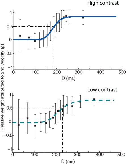
Figure 4. ρn (the relative weight attributed to the post-step velocity) as a function of D (time between velocity change and saccade onset) for a single observer. Dark blue solid line in the top panel denotes the fit of a cumulative Gamma function to the high contrast condition data. Light blue dashed line in the lower panel denotes a Gamma function fit to the low-contrast data. Error bars denote the SD. The dash–dot line in both plots denotes the time at which σn = 0.5, i.e., when both velocities are being weighted equally. Note that while the data are presented here in approximately 15 equal bins, the actual Gamma fit was conducted on the full data set.
More formally, if we think of the velocity change as a step function falling within some temporal filter f(t), then ρn corresponds to the area under f(t) that falls after the velocity change. Therefore, the plot of ρn at a range of values of D gives us the integral of the temporal filter. In order to obtain an estimate of the filter, we fit a reasonable function to these data, and then take its derivative. Note that our actual model fits are based on the data from individual trials, not the binned data which are shown in Figure 4 for illustration purposes only.
We opted for maximum likelihood parameter estimation, because this allows us to perform likelihood-based hypothesis testing of the effects of our experimental manipulation on the various properties of the estimated filter (see below; Burnham and Anderson, 2002; Wagenmakers, 2007). Maximum likelihood requires specification of the probability distribution from which the data points are drawn. This is not straightforward, because it is difficult to know (a) what sources of noise contribute to the variability in the post-step velocity weights and (b) how these noise sources are distributed at any given value for D.
In our previous work (Etchells et al., 2010) we assumed that the two types of endpoint error, εold and εnew, were both Gaussian distributed variables. With the weights defined as a ratio, their probability distribution was described as a ratio of Gaussian densities (Marsaglia, 2006). The parameters of the individual Gaussian components depended on a number of variables that were of minor theoretical interest, such as the mean saccade duration, variability in saccade duration, and variability in saccade landing position. An added complication was that these three quantities could, and to some extent did, vary as a function of D. To limit the number of free parameters we used a kernel estimator for the values of these quantities across the entire range of D and incorporated these estimates in the full expression of the probability distribution of ρ.
We appreciate that this procedure is rather cumbersome, for what appears to be a relatively straightforward and lawful pattern of data. We were therefore keen to develop a simplified method and assess to what extent the estimated velocity weights would be affected by the simplification. In the simplified model, we assume that ρn is Gaussian distributed, with a mean that varies as a function of D according to some functional form (see below). This is the variation that is of primary theoretical interest.
In standard maximum likelihood regression, the SD describes the residuals around the (predicted) mean. It is generally assumed to remain constant and left a free parameter. However, in our case the variability around the (mean) weights clearly varies as a function of D, which can be seen in the size of the error bars in Figure 4. It is important to include this variation: the fit should be most heavily constrained by those data points that were estimated with greater accuracy (i.e., for larger values of D). To make the dependence on D explicit, we write:

We were reluctant to introduce additional free parameters to describe the relation between the SD and time from saccade onset. After all, it is not immediately obvious what function best describes this relation and, more importantly, this relation is not of primary theoretical interest. For this reason, we estimated the SD from the observed values of ρn using a Gaussian kernel, for values of D ranging from 1 to 500 ms. The bandwidth of this smoothing window was set for each observer separately, to whatever bandwidth best captured the distribution of D sampled for that observer. We reasoned that as the variable of interest is sampled as a function of D, a bandwidth for the optimal sampling of D would provide a reasonable window for smoothing the variability in the weights. Specifically, we computed a weighted SD, for every value of D in 1-ms increments:
Here the vector of weights, ω, is the Gaussian smoothing function sampled at 1-ms intervals and μ is the Gaussian-weighted mean.
To capture  we initially chose a scaled cumulative Gamma function. The Gamma function was chosen to accommodate both symmetric and asymmetrical filters, and has frequently been used to describe temporal filters (Watson, 1986; Smith, 1995). The smooth curves in Figure 4 show the fits of the simplified model. These curves are characterized by three free parameters, namely a (the upper asymptote – the lower bound was set to zero), k (shape), and θ (scale). The Nelder–Mead Simplex method (Nelder and Mead, 1965) was used in order to find the set of best-fitting parameters.
It is clear that these functions describe the data well. For each of the 12 data sets reported in the paper (six observers and two contrast levels), we computed the correlation between the predicted weights estimated using the original and simplified fitting methods, for the observed values of D. In all cases the correlation was greater than 0.99. As such, the drastically simplified model results in very similar velocity weighting functions as the more complete (and complex) model developed in our previous work.
Having established the viability of the simplified model, we now turn to the empirical question of interest: what is the effect of contrast on the velocity weighting function? For the data shown in Figure 4, it appears that it takes the system much longer to incorporate the post-step speed into the saccade landing position calculation, as indicated by the more gradual rise to ρn = 1 in the low-contrast condition. For clarity, the dash–dot line in Figure 4 illustrates the point at which the two velocities are being weighed equally (i.e., when ρn = 0.5), showing a shift from ∼190 to ∼230 ms between the high and low-contrast conditions.
Figure 5 shows, for each observer, the derivatives of the weight versus D functions for both contrast conditions. The solid black line shows the filter plot for the high contrast data, and the dashed line shows the filter plot for the low-contrast data. The corresponding shaded regions denote the 95% confidence intervals. These were calculated by producing 1000 bootstrap replications of the fit parameters, using the percentile method (Efron and Tibshirani, 1993).
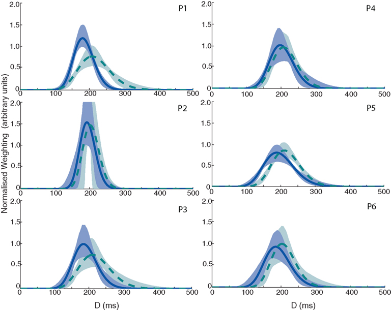
Figure 5. Velocity integration filters for all six observers in Experiment 1. Solid dark blue line denotes the plot based on the high contrast data; dashed light blue line denotes the plot for the low-contrast data. Shaded areas indicate 95% confidence limits based on 10,000 bootstrap replications (dark blue and light green for high and low-contrast conditions, respectively).
The data show that the filter peaks shift toward larger values of D for the low-contrast condition (M = 207 ms, SEM = 1.5 ms) as compared to the high contrast condition (M = 188 ms, SEM = 2.5 ms), for every single observer. There also appears to be a slight increase in the width of the filter as contrast is reduced (M = 79 ms, SEM = 6.7 ms in the high contrast condition, M = 88 ms, SEM = 7.7 ms in the low-contrast condition). These effects are not concomitant with an increase in saccade latency in the step conditions – in the high contrast condition, the mean saccade latency across all observers was 271 ms (SEM = 8.3 ms), compared to a mean saccade latency of 274 ms (SEM = 6.5 ms) in the low-contrast condition – an increase of only 3 ms. The saccade latency should correspond to any changes in the saccadic go signal (i.e., the fixation stimulus change). However, if as a result of the reduction in contrast, it is harder to localize the target (for example, for the purposes of the final position grab), then we might reasonably expect that the saccade latency would increase. The fact that we do not see this is important, as it shows that peak shifts that we see are not simply a result of “stretching” that occurs due to a general increase in the time it takes to detect or generate a saccade to a lower contrast target.
To assess the effects of contrast more formally, we adopted a model selection approach (Burnham and Anderson, 2002; Wagenmakers, 2007). Indeed, this was the motivation for estimating the model parameters using maximum likelihood. For this purpose, we defined a number of competing models that represent different hypotheses about the effect(s) of contrast. The likelihoods of these models constitute an index of the amount of evidence provided by the data for the different hypotheses.
The following four competing models were defined. If contrast had no effect on the width or peak location of the filter, we would expect a set of four parameters to suffice – a single peak location parameters, a width parameter, and two separate asymptotes (this is hereafter known as the baseline model). At the other extreme, contrast could affect every possible aspect of the filter, necessitating two separate sets of three parameters to account for the data. We refer to this model as the saturated model. In between these two extremes fall two reduced models of critical interest: (1) a five-parameter peak location model accommodates the data from both contrast conditions with a common width, but allows the location and asymptote to vary with contrast; (2) a five-parameter width model which assumes different widths and asymptotes for the low and high contrasts. In other words, we force the location and/or widths to be the same.
One problem with the Gamma function is that its parameters do not correspond to experimentally interesting parameters such as filter width and peak position. This makes it very difficult to, for example, test the competing models that we have outlined above. Therefore, for the purpose of this test, we chose to fit our data with scaled cumulative Gaussian curves, instead of the Gamma functions used earlier. As can be seen in Figure 5, the identified temporal filters are relatively symmetrical. Seeing as this is the case, a Gaussian function is attractive because its two parameters are independent and correspond directly to the location and width parameters of the filter. In comparison, the shape and scale parameters of the Gamma interact to jointly determine its location and width. The inability of the Gaussian to accommodate the slight asymmetries in the filters, did result in a decreased goodness-of-fit, as we will show below. However, the critical components of the filter, the width and location, were numerically very close under both models. Moreover, the effect(s) of contrast on these two components was also very similar when estimated with Gaussian or Gamma functions. For this reason, we see the reduction in goodness-of-fit as a price worth paying for the greater utility of the Gaussian function in terms of parameter interpretation.
Finally, the four models defined above differ in the number of free parameters. In evaluating their likelihoods, it is desirable to take this variation in complexity into account. A Bayesian information criterion (BIC) adjusts the log-likelihood of a model, given the observed data and best-fitting parameters, according to the number of free parameters (Schwarz, 1978; Wagenmakers, 2007). In particular:

where L is the maximum log-likelihood, k is the number of free parameters of a model, and N is the number of observed data points. As is readily apparent from Eq. 4, the BIC balances goodness-of-fit with parsimony. Models with smaller BICs are more competitive, as those with a greater number of free parameters (which should produce a better fit) are penalized.
Table 1 shows the values of the BICs for all four models and observers, the summed totals across the sample, as well as the BICs for the fits of the saturated Gamma functions for each observer. The Gamma function is the clear overall winner with the lowest BIC – the BIC difference with the saturated Gaussian model is 41, which corresponds to a corrected likelihood-ratio, or Bayes factor, of greater than 1000 (Wagenmakers, 2007). Thus it is clear that fitting the data with a Gaussian function results in a less desirable fit of the data; however, the Gaussian still offers a considerable advantage in terms of the interpretability of the parameters. Moreover, inspection of a plot of the weightings based on the best-fitting Gaussian and Gamma (both full and simplified versions) models shows that all three functions fit the data reasonably well (see Figure 6).
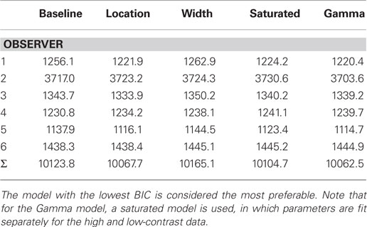
Table 1. Bayesian Information Criterions (and summed BICs) for all six observers for each of the four Gaussian comparison models.
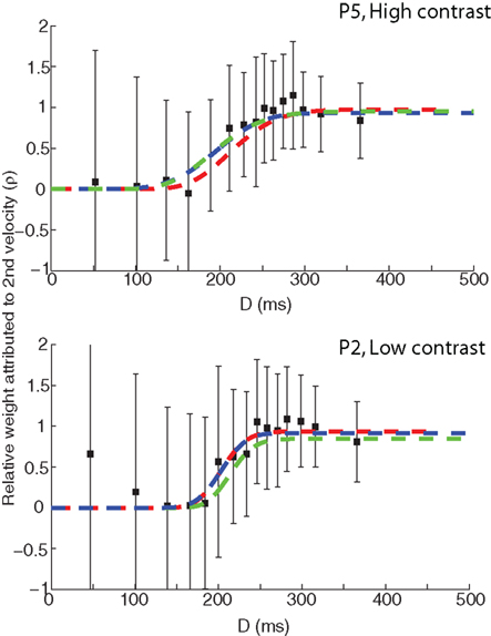
Figure 6. Comparison of the weighting function fits based on the original Gamma model (green), the simplified Gamma model (red), and a Gaussian (blue). The top panel shows the participant data set with the highest correlation between the model fits (P5).The bottom panel shows the participant data set with the lowest correlation between the model fits (P2).
With respect to the Gaussian model comparisons then, the five-parameter location model is the winning model by a clear margin. In other words, allowing a peak shift, but not a width shift, provides the best description of the data. The BIC difference with the nearest competitor – the saturated Gaussian model – is ∼37, which again corresponds to a Bayes factor, of greater than 1000. The direct comparison between the width and location models also came out strongly in favor of the location model (a combined BIC difference of almost 100). In both circumstances, the size of the Bayes factor corresponds to an effective p value of <0.01 (Wagenmakers, 2007). In conclusion, it seems unlikely that allowing the width of the integration filters to vary with contrast improves our model fits in any meaningful way – it is the location of the peak of the filter that is important. Across all six observers, this shift in μ corresponded to a peak shift of 18 ms as contrast is reduced, comparable to the shift found for the Gamma fits.
Discussion
Sensorimotor decisions in a dynamic world necessarily involve an element of prediction. Behavior needs to be adapted to the future characteristics of the targeted object (e.g., its position). Careful analysis of variable single-trial behavior in response to a perturbation of the sensory input affords insight over what interval the relevant object characteristics are estimated. In the present study, we simplified and adjusted our method (Etchells et al., 2010) for identifying the temporal filter that is used by observers to estimate the velocity of a moving object. This estimate then guides the observers’ prediction about the future location of the object, taking into account the interval between the decision to move and the completion of that movement.
Single cell recording in the primate brain and VEP studies in humans generally suggest an increase in conduction latency with lower contrast (e.g., Shapley and Victor, 1978; Kuba and Kubova, 1992; Kubova et al., 1995; Bach and Ullrich, 1997). Moreover, neuronal conduction latencies generally increase in higher cortical areas (for example, in MT and beyond) as successive stages of processing are added (Raiguel et al., 1999), and this effect will be amplified by a reduction in contrast. Behavioral studies have often measured reaction times, either of manual button presses (e.g., Mansfield, 1973; Breitmeyer, 1975; Harwerth and Levy, 1978; Plainis and Murray, 2000; Murray and Plainis, 2003)or saccades (Carpenter, 2004; Ludwig et al., 2004; Taylor et al., 2006; White et al., 2006). Generally speaking, reductions in contrast diminish the behavioral responsiveness to changes in the stimulus.
However, to get from the brain and responses of single cells to general behavior requires postulating internal information processing mechanisms. For the case of intercepting moving targets, any reduced behavioral responsiveness to velocity changes at low-contrast could come about either through a widening of the temporal filter used to estimate instantaneous velocity, and/or through a delay in the input to the integration mechanism. It was by no means obvious a priori which mechanism(s) would be responsible for diminished visual–saccadic performance. Our analysis method allowed us to distinguish between these possibilities. We obtained strong evidence in favor of a shift of the filter toward longer latencies, most likely produced by the longer input delays reviewed above. We found no evidence in favor of a consistent increase in the width of the filters at the lower contrast level.
Whilst our method cannot tell us where velocity integration for saccadic planning resides in the brain, it would not be unreasonable to suggest area MT as a likely candidate. Area MT is important for motion integration (Born and Bradley, 2005), and is known to project to eye movement related structures such as the superior colliculus (Ungerleider et al., 1984) and frontal eye fields (Tian and Lynch, 1996; Leigh and Zee, 2006). As noted above, lowering the contrast of moving visual stimuli results in an increase in the time that it takes for signals to reach MT (e.g., Kubova et al., 1995; Bach and Ullrich, 1997). It would be a matter for future research, perhaps using imaging techniques, in order to determine the likely cortical location of this mechanism.
Using a closely related approach, Tavassoli and Ringach (2009) identified the temporal filter driving eye velocity during smooth pursuit. Their pursuit stimulus was perturbed with Gaussian velocity noise. By correlating the velocity of the noisy stimulus with the eye velocity at different lags, they were able to estimate the latency with which the system responds to a perturbation, as well as the interval over which velocity information was integrated. For a large reduction in target contrast comparable to that of the current study (although note that their lowest contrast level was lower than ours), the filters showed a shift in the time-to-peak on the order of ∼30 ms. In addition, they also found a moderate increase in the width of the filters of ∼20. Given the evidence for shared visual processing between the pursuit and saccadic systems (Liston and Krauzlis, 2005; Orban de Xivry and Lefèvre, 2007), it would be reasonable to suggest that any neuronal effects of target speed estimation on smooth pursuit might also be reflected in the saccadic system. Indeed, one of the major inputs shared between the two systems appears to be target velocity (e.g., Newsome et al., 1985; Gellman and Carl, 1991; de Brouwer et al., 2002).
Given that lowering the contrast of a stimulus results in a decrease in the SNR (e.g., Weiss et al., 2002), we expected that a widening of the temporal filters might be a useful way in which to counteract this decrease. One reason that we did not see this decrease is that the contrast level we used in the low-contrast condition was simply not close enough to threshold for it to cause real issues with the SNR. Additionally, widening the integration epoch in order to boost the SNR of the internal velocity estimate may only be adaptive in situations where the velocity remains (approximately) constant. In realistic terms, moving objects are often subject to changes in velocity. In such an environment, widening the temporal filter might not be useful, as it would hinder the fidelity with which the observer could track changes in velocity, and ultimately result in less accurate estimates of how fast a target is moving. In our present study, observers are presented with a mix of constant velocity and changing velocity trials. Importantly, the velocity change was relatively large (e.g., compared to the zero-mean noise used in Tavassoli and Ringach, 2009). It may be that the cost of widening the filter under these conditions was simply too large. The necessity for rapidity of response might well have outweighed any need for increasing the SNR. Note that if this explanation is correct, it suggests a degree of flexibility in the system so that adaptation of the integration period depends on the wider context in which the system operates.
The methodology that we present here sits well within the broader context of research assessing perceptual and decision-making behavior on single trials. Using a relatively simple experimental paradigm (i.e., tracking primary orienting eye movements to a moving target), quite complex and temporally precise knowledge about how visual information is used within the saccadic latency period can be gathered. By varying target contrast and the timing of the saccadic go signal from trial-to-trial, we are able to show not only that the integration of visual (in this case, velocity) information can be modified during the latency period, but we are also able to show how it is modified. By assessing these results within the context of similar studies (e.g., Caspi et al., 2004; Ludwig et al., 2005), we can build up a coherent picture about the time course of how eye movement decisions are made using simple behavioral paradigms. This allows for a great deal of flexibility in the methods and models that are implemented, and allows for simple modifications in order to answer further questions about what exactly occurs during the saccadic latency period. For example, the use of non-constant velocities in the present experiment would aid in the assessment of how the integration filters deal with acceleration. In turn, this may provide an understanding as to how acceleration is represented within areas such as MT (e.g., Schlack et al., 2007, 2008), and also how sampling mechanisms are used in the predict drive for ocular pursuit (see Bennett et al., 2007). Along more general lines, such approaches may help to further our understanding of how the smooth pursuit and saccadic systems interact and coordinate with each other.
Conclusion
The simplified methodology presented in this paper provides a novel addition to a growing toolbox for the behavioral study of how information on single trials may be integrated and used in eye movement programming. Our approach allows for maximum likelihood estimates of the parameters of the temporal filter that best accounts for the interval over which the saccadic system samples the velocity of a moving target. The likelihoods provide a solid basis upon which to assess the significance of experimentally targeted variables, such as contrast in this study. More generally, we believe this methodology more uniquely constrains internal processing mechanisms that transform sensory inputs into motor outputs, linking brain and behavior.
Conflict of Interest Statement
The authors declare that the research was conducted in the absence of any commercial or financial relationships that could be construed as a potential conflict of interest.
References
Aslin, R. N., and Shea, S. L. (1987). The amplitude and angle of saccades to double-step target displacements. Vision Res. 27, 1925–1942.
Bach, M., and Ullrich, D. (1997). Contrast dependency of motion-onset and pattern-reversal VEPs: interaction of stimulus type, recording site and response component. Vision Res. 37, 1845–1849.
Becker, W., and Jürgens, R. (1979). An analysis of the saccadic system by means of double-step stimuli. Vision Res. 19, 967–983.
Bennett, S. J., Orban de Xivry, J. J., Barnes, G. R., and Lefèvre, P. (2007). Target acceleration can be extracted and represented within the predictive drive to ocular pursuit. J. Neurophysiol. 98, 1405–1414.
Benton, C. P., and Curran, W. (2009). The dependence of perceived speed upon signal intensity. Vision Res. 49, 284–286.
Beutter, B. R., Eckstein, M. P., and Stone, L. S. (2003). Saccadic and perceptual performance in visual search tasks. I. Contrast detection and discrimination. J. Opt. Soc. Am. A Opt. Image Sci. Vis. 20, 1341–1355.
Born, R. T., and Bradley, D. C. (2005). Structure and function of visual area MT. Annu. Rev. Neurosci. 28, 157–189.
Breitmeyer, B. G. (1975). Simple reaction time as a measure of the temporal response properties of transient and sustained channels. Vision Res. 15, 1411–1412.
Burnham, K. P., and Anderson, D. R. (2002). Model Selection and Inference: A Practical Information-Theoretic Approach. New York: Springer.
Carpenter, R. H. S. (2004). Contrast, probability and saccadic latency: evidence for independence of detection and decision. Curr. Biol. 14, 1576–1580.
Caspi, A., Beutter, B. R., and Eckstein, M. P. (2004). The time course of visual information accrual guiding eye movement decisions. Proc. Natl. Acad. Sci. U.S.A. 101, 13086–13090.
Cornelissen, F. W., Peters, E. M., and Palmer, J. (2002). The eyelink toolbox: eye tracking with MATLAB and the psychophysics toolbox. Behav. Res. Methods Instrum. Comput. 34, 613–617.
de Brouwer, S., Missal, M., Barnes, G., and Lefèvre, P. (2002). Quantitative analysis of catch-up saccades during sustained pursuit. J. Neurophysiol. 87, 1772–1780.
Eckstein, M. P., Beutter, B. R., Pham, B. T., Shimozaki, S. S., and Stone, L. S. (2007). Similar neural representations of the target for saccades and perception during search. J. Neurosci. 27, 1266–1270.
Efron, B., and Tibshirani, R. J. (1993). An Introduction to the Bootstrap. Monographs on Statistics and Applied Probability. Boca Raton, FL: Chapman & Hall/CRC.
Enroth-Cugell, C., and Robson, J. G. (1966). The contrast sensitivity of retinal ganglion cells of the cat. J. Physiol. 187, 517–552.
Etchells, P. J., Benton, C. P., Ludwig, C. J. H., and Gilchrist, I. D. (2010). The target velocity integration function for saccades. J. Vis. 10, 1–14.
Findlay, J. M., and Harris, L. R. (1984). “Small saccades to double-stepped targets moving in two dimensions,” in Theoretical and Applied Aspects of Eye Movement Research, eds A. G. Gale and F. Johnson (Amsterdam: Elsevier), 71–78.
Gellman, R. S., and Carl, J. R. (1991). Motion processing for saccadic eye movements in humans. Exp. Brain Res. 84, 660–667.
Glimcher, P. W. (2001). Making choices: the neurophysiology of visual-saccadic decision making. Trends Neurosci. 24, 654–659.
Gold, J. I., and Shadlen, M. N. (2001). Neural computations that underlie decisions about sensory stimuli. Trends Cogn. Sci. 5, 10–16.
Gold, J. I., and Shadlen, M. N. (2007). The neural basis of decision making. Annu. Rev. Neurosci. 30, 535–574.
Harwerth, R. S., and Levy, D. M. (1978). Reaction time as a measure of suprathreshold grating detection. Vision Res. 18, 1579–1586.
Kaplan, E., and Shapley, R. M. (1982). X and Y cells in the lateral geniculate nucleus of macaque monkeys. J. Physiol. 330, 125–143.
Kerzel, D., and Gegenfurtner, K. R. (2003). Neuronal processing delays are compensated in the sensorimotor branch of the visual system. Curr. Biol. 13, 1975–1978.
Krekelberg, B., van Wezel, R. J., and Albright, T. D. (2006). Interactions between speed and contrast tuning in the middle temporal area: implications for the neural code for speed. J. Neurosci. 26, 8988–8998.
Kuba, M., and Kubova, Z. (1992). Visual evoked potentials specific for motion-onset. Doc. Ophthalmol. 80, 83–89.
Kubova, Z., Kuba, M., Spekreijse, H., and Blakemore, C. (1995). Contrast dependence of motion-onset and pattern-reversal evoked potentials. Vision Res. 35, 197–205.
Liston, D., and Krauzlis, R. J. (2005). Shared decision signal explains performance and timing of pursuit and saccadic eye movements. J. Vis. 5, 678–689.
Livingstone, M. S., and Conway, B. R. (2006). Contrast affects speed tuning, space-time slant, and receptive-field organisation of simple cells in macaque V1. J. Neurophysiol. 97, 849–857.
Ludwig, C. J. H. (2009). Temporal integration of sensory evidence for saccade target selection. Vision Res. 49, 2764–2773.
Ludwig, C. J. H., Gilchrist, I. D., and McSorley, E. (2004). The influence of spatial frequency and contrast on saccade latencies. Vision Res. 44, 2597–2604.
Ludwig, C. J. H., Gilchrist, I. D., McSorley, E., and Baddeley, R. J. (2005). The temporal impulse response underlying saccadic decisions. J. Neurosci. 25, 9907–9912.
Ludwig, C. J. H., Mildinhall, J. W., and Gilchrist, I. D. (2007). A population coding account for systematic variation in saccadic dead time. J. Neurophysiol. 97, 795–805.
Maunsell, J. H. R., Ghose, G. M., Assad, J. A., McAdams, C. J., Boudreau, C. E., and Noerager, B. D. (1999). Visual response latencies of magnocellular and parvocellular LGN neurons in macaque monkeys. Vis. Neurosci. 16, 1–14.
Murray, I. J., and Plainis, S. (2003). Contrast coding and magno/parvo segregation revealed in reaction time studies. Vision Res. 43, 2707–2719.
Nelder, J. A., and Mead, R. (1965). A simplex-method for function minimization. Comput. J. 7, 308–313.
Newsome, W. T., Wurtz, R. H., Dursteler, M. R., and Mikami, A. (1985). Deficits in visual-motion processing following ibotenic acid lesions of the middle temporal visual area of the macaque monkey. J. Neurosci. 5, 825–840.
Nickerson, R. S., and Burnham, D. W. (1969). Response times with nonaging foreperiods. J. Exp. Psychol. 79, 452–457.
Nummela, S. U., Lovejoy, L. P., and Krauzlis, R. J. (2008). Saccade selection when reward probability is dynamically manipulated using Markov chains. Exp. Brain Res. 187, 321–330.
Orban de Xivry, J. J., and Lefèvre, P. (2007). Saccades and pursuit: two outcomes of a single sensorimotor process. J. Physiol. 584, 11–23.
Oswal, A., Ogden, M., and Carpenter, R. H. S. (2007). The time course of stimulus expectation in a saccadic decision task. J. Neurophysiol. 97, 2722–2730.
Pack, C. C., Hunter, J. N., and Born, R. T. (2005). Contrast dependence of suppressive influences in cortical area MT of alert macaque. J. Neurophysiol. 93, 1809–1815.
Plainis, S., and Murray, I. J. (2000). Neurophysiological interpretation of human visual reaction times: effect of contrast, spatial frequency and luminance. Neuropsychologia 38, 1555–1564.
Raiguel, S. E., Xiao, D. K., Marcar, V. L., and Orban, G. A. (1999). Response latency of macaque area MT/V5 neurons and its relationship to stimulus parameters. J. Neurophysiol. 82, 1944–1956.
Schall, J. D. (2003). Neural correlates of decision processes: neural and mental chronometry. Curr. Opin. Neurobiol. 13, 182–186.
Schlack, A., Krekelberg, B., and Albright, T. D. (2007). Recent history of stimulus speeds affects the speed tuning of neurons in area MT. J. Neurosci. 27, 11009–11018.
Schlack, A., Krekelberg, B., and Albright, T. D. (2008). Speed perception during acceleration and deceleration. J. Vis. 8, 1–11.
Seijas, O., Gómez de Liaño, P., Gómez de Liaño, R., Roberts, C. J., Piedrahita, E., and Diaz, E. (2007). Ocular dominance diagnosis and its influence in monovision. Am. J. Ophthalmol. 144, 209–216.
Shapley, R. M., and Victor, J. D. (1978). The effect of contrast on the transfer properties of cat retinal ganglion cells. J. Physiol. 285, 275–298.
Smith, P. L. (1995). Psychophysically principled models of visual simple reaction time. Psychol. Rev. 102, 567–593.
Spering, M., Kerzel, D., Braun, D. I., Hawken, M. J., and Gegenfurtner, K. R. (2005). Effects of contrast on smooth pursuit eye movements. J. Vis. 5, 455–465.
Tavassoli, A., and Ringach, D. L. (2009). Dynamics of smooth pursuit maintenance. J. Neurophysiol. 102, 110–118.
Taylor, M. J., Carpenter, R. H. S., and Anderson, A. J. (2006). A noisy transform predicts saccadic and manual reaction times to changes in contrast. J. Physiol. 573, 741–751.
Tian, J. R., and Lynch, J. C. (1996). Corticocortical input to the smooth and saccadic eye movement subregions of the frontal eye field in the Cebus monkey. J. Neurophysiol. 76, 2754–2771.
Ungerleider, L. G., Desimone, R., Galkin, T. W., and Mishkin, M. (1984). Subcortical projections of area MT in the macaque. J. Comp. Neurol. 223, 368–386.
Wagenmakers, E. J. (2007). A practical solution to the pervasive problems of p values. Psychon. Bull. Rev. 14, 779–804.
Walker, R., Walker, D. G., Husain, M., and Kennard, C. (2000). Control of voluntary and reflexive saccades. Exp. Brain Res. 130, 540–544.
Watson, A. B. (1986). “Temporal sensitivity,” in Handbook of Perception and Human Performance, eds K. R. Boff, L. Kaufman, and J. P. Thomas (New York: Wiley), 6.1–6.43.
Weiss, Y., Simoncelli, E. P., and Adelson, E. H. (2002). Motion illusions as optimal percepts. Nat. Neurosci. 5, 598–604.
Keywords: saccades, contrast, velocity integration, motion, prediction
Citation: Etchells PJ, Benton CP, Ludwig CJH, and Gilchrist ID (2011) Testing a simplified method for measuring velocity integration in saccades using a manipulation of target contrast. Front. Psychology 2:115. doi: 10.3389/fpsyg.2011.00115
Received: 02 March 2011;
Paper pending published: 03 May 2011;
Accepted: 16 May 2011;
Published online: 26 May 2011.
Edited by:
Paul Sajda, Columbia University, USAReviewed by:
Roberto Caldara, University of Glasgow, UKPiers D. L. Howe, Harvard Medical School, USA
Copyright: © 2011 Etchells, Benton, Ludwig and Gilchrist. This is an open-access article subject to a non-exclusive license between the authors and Frontiers Media SA, which permits use, distribution and reproduction in other forums, provided the original authors and source are credited and other Frontiers conditions are complied with.
*Correspondence: Peter J. Etchells, School of Experimental Psychology, University of Bristol, 12A Priory Road, Clifton, Bristol BS8 1TU, UK. e-mail:cGV0ZXIuZXRjaGVsbHNAYnJpc3RvbC5hYy51aw==