- 1 Centre de Recherche Cerveau et Cognition, Paul Sabatier University, Toulouse, France
- 2 Centre de Recherche Cerveau et Cognition, UMR5549, CNRS, Toulouse, France
- 3 Swartz Center for Computational Neuroscience, Institute for Neural Computation, University of California San Diego, La Jolla, CA, USA
In electroencephalography, the classical event-related potential model often proves to be a limited method to study complex brain dynamics. For this reason, spectral techniques adapted from signal processing such as event-related spectral perturbation (ERSP) – and its variant event-related synchronization and event-related desynchronization – have been used over the past 20 years. They represent average spectral changes in response to a stimulus. These spectral methods do not have strong consensus for comparing pre- and post-stimulus activity. When computing ERSP, pre-stimulus baseline removal is usually performed after averaging the spectral estimate of multiple trials. Correcting the baseline of each single-trial prior to averaging spectral estimates is an alternative baseline correction method. However, we show that this method leads to positively skewed post-stimulus ERSP values. We eventually present new single-trial-based ERSP baseline correction methods that perform trial normalization or centering prior to applying classical baseline correction methods. We show that single-trial correction methods minimize the contribution of artifactual data trials with high-amplitude spectral estimates and are robust to outliers when performing statistical inference testing. We then characterize these methods in terms of their time–frequency responses and behavior compared to classical ERSP methods.
Introduction
Electroencephalography and magnetoencephalography methods have become standard tools to study brain mechanisms. Different approaches have been used to unveil brain electrical activity in relation to sensory, motor, or cognitive events using electrical potential variations recorded either at the scalp level or from intra-cranial electrodes. The study of changes of the ongoing electroencephalogram (EEG) in response to stimulation started with event-related potentials (ERP) techniques, which relies on measuring the amplitude and latency of post-stimulus peaks in stimulus-locked EEG trial averages. The standard ERP model relies on the hypothesis that ERPs consist of stereotyped patterns of stimulus-locked electrical activity, superimposed onto an independent stationary stochastic EEG processes (Basar and Dumermuth, 1982; Luck, 2005; Nunez and Srinivasan, 2006). In the ERP model, every single-trial contains a noisy version of the grand average ERP, and, when averaging trials, “stationary” or “non-time-locked” background EEG elements of the signal cancel out.
The standard ERP model has been intensely debated for the past 10 years. In some rare cases, the standard ERP model may hold in particular for early pre-perceptual activity such as somatosensory evoked potentials with latencies as short as 20 ms (N20 wave; Yao and Dewald, 2005; Kennett et al., 2011). However, in most cases, including the well-known P300 ERP peak, scalp ERPs arise as a complex superposition of ongoing EEG activity in single-trials (Delorme et al., 2007). Most ERP peaks have been shown to result from a reorganization of the phase of ongoing EEG oscillations (Tallon-Baudry et al., 1996; Delorme et al., 2002; Makeig et al., 2002). Thus the phase or latency of the ERP peak in single-trials is not constant but may depend on the ongoing EEG activity (Makeig et al., 2004). Since the ERP by itself cannot unravel complex EEG dynamics, it became necessary to develop new techniques.
In the 1960s, while some researchers were starting to use ERPs, some other pioneer researchers were using pure-frequency based techniques to assess spontaneous EEG oscillatory changes under various conditions. Scientists compared the EEG spectrum of subjects with their eyes opened or their eyes closed, and observed an increased 10-Hz alpha power in the eyes-closed condition (Legewie et al., 1969). This approach focused on the frequency domain exclusively while the ERP approach focused only on the time domain. In the last 20 years, evolution of computational capabilities brought up the possibility of developing new methods to visualize, quantify, and characterize stimulus-induced complex brain dynamic simultaneously in the time and frequency domains. These new tools allow disentangling ongoing brain activity from stimulus-evoked activity.
These new post-stimulus spectral estimation methods were called event-related desynchronization (ERD; Pfurtscheller and Aranibar, 1977), event-related synchronization (ERSyn; Pfurtscheller, 1992), and event-related spectral perturbation (ERSP; Makeig, 1993; Makeig et al., 2004) which regroups both ERSyn and ERD. The concept of ERD, ERSyn, and ERSP consists in averaging the power spectrum of short sliding time windows in multiple stimulus-locked data trials. ERSP results are usually visualized in 2-D time–frequency images where the pixels’ color represent power variations at different time–frequency points.
Using ERSP is however not as simple as using ERP since there are a large number of variants. For example, it is possible to compute power using either fast Fourier transform (FFT) or Wavelet transforms (Delorme and Makeig, 2004). Wavelets also have different variants. Although most authors use Morlet wavelets (Schiff et al., 1994; Tallon-Baudry et al., 1997; Herrmann et al., 1999; Adeli et al., 2003; Lemm et al., 2004), EEG has been studied with other type of wavelets such as Daubechies or Meyer wavelets (Bertrand et al., 1994; Kim et al., 2008; Asaduzzaman et al., 2010). In addition, it is also possible to compute ERSPs using the multi-taper method (Mitra and Pesaran, 1999) or band-passed Hilbert transforms (Clochon et al., 1996). Fortunately, all of these spectral methods tend to return similar results (Le Van Quyen et al., 2001; Bruns, 2004) so we will focus on using simple sliding-window FFT decompositions in this report.
In addition to using different spectral methods, ERSP variants may also use different baseline correction methods. When processing intra-cranial electrodes, researchers often avoid computing baselines and analyze raw time-varying spectral power variations (Tallon-Baudry et al., 2001). This is possible because intra-cranial EEG data is less subject to noise than scalp EEG recordings and event-related spectral variations may be visible without any further processing. However, when using scalp channels, it is often necessary to subtract baseline activity in each frequency band from the post-stimulus period. Intra-cranial EEG, scalp EEG, or Magneto-encephalography (MEG) raw spectral images are dominated by low frequencies (Freeman et al., 2000; Slotnick et al., 2002) which can mask the activity at higher frequencies. Moreover, even within a given frequency band, post-stimulus power changes relative to the pre-stimulus baseline period are often subtle and may be difficult to observe (Figure 1). Thus it becomes necessary to compute spectral changes relative to baseline. Since most of EEG spectral analysis aims to quantify the effect of a stimulus on the ongoing EEG spectrum, the most intuitive approach to isolate event-related changes is to subtract the trial-averaged pre-stimulus spectral activity from post-stimulus activity in each frequency band. Eventually, baseline correction may also be useful when performing statistical inference where post-stimulus activity is compared to baseline activity.
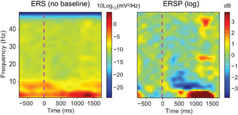
Figure 1. Raw event-related spectrum (absolute log-ERS) on the left versus baseline corrected ERSP (log-ERSP) on the right for scalp EEG data trials. Electrode Iz from the “animal” dataset of subject “CLM” (see Materials and Methods) was used to compute FFT-based ERS and ERSP. ERS was computed using Eq. 1and log-ERSP was computed using the classical baseline correction divisive method described in Eq. 6(see Materials and Methods). Although post-stimulus power decrease at about 7 Hz is clearly visible on the ERSP image, it is more difficult to see in the ERS image where large low-frequency changes stretch the color scale limits. This shows the usefulness of removing the pre-stimulus baseline for scalp EEG data.
There are mainly two methods to perform baseline correction. These two methods rely on different assumptions about the EEG signal. The first method assumes an additive model where stimulus-induced power at specific frequencies adds onto existing power at these frequencies. The second alternative model consists in using a divisive baseline, which assumes an EEG gain model where the occurrence of a stimulus proportionally increases or decreases the amplitude of existing oscillatory EEG activity. Both models are widely used and, for the first time, we are comparing them in terms of their time–frequency response and behavior when performing statistical inference testing.
Finally, a new idea we are introducing here deals with trial-based baseline correction methods. The classical baseline approach involves first computing time–frequency decompositions for each trial, then computing a trial average, and as a last step removing the pre-stimulus baseline. However, as we show in this report, this method proves to be quite sensitive to noisy data trials. By contrast, it is also possible to perform different types of correction in single-trials prior to averaging time–frequency estimates. In this report, we compare new trial-based baseline correction approaches to classical baseline correction methods. We will demonstrate how our trial-based correction methods tend to make ERSP less sensitive to the presence of a limited number of trials with excessive ambient or physiological noise.
Materials and Methods
We will first describe the two different models used to compute ERSP for both the classical baseline correction approach and the single-trial baseline correction approach. We will then detail the two statistical methods implemented to compute significance. Finally, we will explain the procedure used to study ERSP robustness to noisy trials.
ERSP Models
Two main methods for ERSP pre-stimulus baseline correction may be distinguished. We first present these two approaches, which for simplicity we have termed the ERSP “gain model” and the ERSP “additive model”. We describe how ERSPs are calculated for each of these models and then show how they can be adapted for single-trial baseline correction.
Event-related spectrum
The event-related spectrum (ERS) consists in computing the data power spectrum for sliding time windows centered at time t in each trial and then computing the average across trials. The mean ERS for frequency f and time point t is defined as

where n is the total number of trials, and Fk( f,t) is the spectral estimate at frequency f and time point t for trial k. In the rest of this report, we assume that Fk( f,t) is computed using FFT after applying a Hanning window to remove window border effects. However, formula (1) is still valid if Fk( f,t) represents a wavelet or a Hilbert transform. Formula (1) would have to be modified for multi-taper decompositions (Mitra and Pesaran, 1999).
Classical baseline approaches
Classical baseline normalization – additive model. The first method to remove baseline activity presented here is based on an additive ERSP model, which assumes that stimulus-induced spectral activity adds linearly to existing pre-stimulus spectral activity. This approach was first introduced by Tallon-Baudry et al. (1996, 1999) and is now one of the standard approaches for computing ERSPs.
To compute this ERSP, the ERS trial average is normalized for each frequency band. In the baseline period – classically defined as the period preceding the stimulus – the average and standard deviation (SD) of power are first computed at each frequency. Then, the average baseline power is subtracted from all time windows at each frequency, and the resulting baseline-centered values are divided by the SD. For each time–frequency point of the time–frequency decomposition, the calculation of the ERSP can be formalized as follows:

where μB( f ) is the mean spectral estimate for all baseline points at frequency f

where B is the ensemble of time points in the baseline period and m is the cardinal of B or the total number of time points in the baseline period. σB( f ) is the spectral estimate SD for all baseline points at frequency f and is defined as:

The unit for ERSPz values computed in Eq. 2is z-score or SD of the baseline. A close variant to this approach is the mean baseline removal approach, which consists in simply removing the mean baseline value at each frequency. Because of the way significance is computed (see Statistical Methods to Assess Significance), we would not observe any difference between ERSPz and the mean baseline removal approach in terms of region of significance. It will therefore not be included in this report.
Dividing by baseline value – gain model. The gain model is detailed in Delorme and Makeig (2004) and is the default model in the popular EEGLAB software. In this model, for each frequency band, ERS power at each time–frequency point is divided by the average spectral power in the pre-stimulus baseline period at the same frequency. Two measures may be derived from this model, an absolute ERSP measure and a log-transformed ERSP measure. The absolute ERSP measure is computed as follows:

where μB( f ) is the mean spectral estimate defined in Eq. 3. The unit for ERSP% is percentage of baseline activity. The log-transformed measure is derived by taking the log value of ERSP%:

The logarithmic scale of the last measure offers two advantages compared to the methods described previously. First, it has been shown by a large body of statistical signal processing literature that, for skewed signals such as EEG, the distribution of the logarithm of the signal is more normal than the distribution of the original signal. Therefore parametric inference testing is often more valid when applied to log-transformed power values – although in the case of the EEGLAB software, which we are using in this report, most statistics rely on surrogate methods which are not sensitive to the data probability distribution. The second advantage of logarithmic scales is that they allow visualizing a wider range of power variations, whereas for the absolute scales, power changes at low frequencies may mask power changes at high frequencies.
By definition, the unit of ERSPlog is Decibel (dB). Both measures ERSP% and ERSPlog are commonly used in the literature (Fuentemilla et al., 2006; Delorme et al., 2007; Meltzer et al., 2008).
Single-trial baseline correction
In the previous section we outlined different types of ERSP calculations applied to the ERS trial average. In this section, we are introducing methods to compute single-trial baseline correction. For each of the two ERSP models, namely the “additive model” and the “gain model,” the single-trial version of calculation is formalized below.
Single-trial baseline normalization – additive model. Instead of computing baseline normalization after trial averaging, baseline normalization is computed for each trial using the following equations:


where μ′B ( f,k) is the mean baseline spectral estimate for trial k at frequency f and is defined as

σ′B ( f,k) is the spectral estimate SD for the baseline period of trial k at frequency f and is defined as

Dividing single-trials by their baseline value – gain model. In the case of the gain model, we first divide each time–frequency point value by the average spectral power in the pre-stimulus baseline period at the same frequency. It is only after each trial has been baseline corrected that we compute the trial average. This is summarized in the following formal equations:


where μ′B ( f,k) is the mean baseline spectral estimate for trial k at frequency f described in Eq. 9.
The log-transformed ERSP version is computed by taking the logarithm of ERSPTB − %

Note that it would also be possible to compute the log of each trial and then average the results – which would be equivalent to computing the product of the time–frequency estimates across trials and then performing a log-transformation as:

However, calculating the product of single-trial spectral estimates might not be biological plausible. Moreover, it also leads to regularization issues. When the mean baseline power at a given frequency is too close to 0, the term defined in (11) would tend toward infinite. As a consequence, after log-transformation, the power of some trials could dominate the ERSP. This last approach has therefore not been considered in this report.
Classical pre-stimulus baseline after full-epoch length single-trial correction. There is no need to perform classical baseline correction after single-trial baseline correction since, after single-trial pre-stimulus baseline correction, averaging values across trials preserves the baseline value. For instance, the baseline value for each trial is already centered at 0 for the ERSPTB − z measure – after averaging trials the average baseline value remains 0. Similarly the average baseline value is 1 in ERSPTB − %, and remains 1 after averaging trials.
This is important when computing statistics since the NULL hypothesis is based on trial-average baseline values: the general NULL hypothesis states that post-stimulus values do not differ from baseline values. Having a centered baseline is especially important for the “Bootstrap random polarity inversion” statistical method (see Statistical Methods to Assess Significance) that randomly inverts baseline corrected single-trial spectral estimate polarity at each time–frequency point.
In the results section, we show that single-trial baseline correction methods are biased. As a consequence we developed methods that normalize single-trials or centers them at 1 prior to applying standard baseline correction methods. We call these methods full-epoch length single-trial corrections, which, as we will see in the Section “Results,” proved to be powerful techniques. Full-epoch length single-trial correction is equivalent to computing ERSPTB − z, ERSPTB − %, or ERSPTB − log and consider the full-trial length for the “baseline” period instead of the pre-stimulus baseline. Note that the term “baseline” is not appropriate any longer in this case and is simply used to outline the calculation method. After computing ERSP trial averages, the average pre-stimulus values (actual pre-stimulus baseline) may differ from 0 (ERSPTB − z, ERSPTB − log) or from 1 (ERSPTB − %). It is therefore important to recompute the classical trial average pre-stimulus baseline prior to computing statistics. This is formalized in the following paragraph: it consists in first performing full-epoch length single-trial correction, and then performing classical pre-stimulus baseline corrections on the resulting ERSP trial averages.
ERSPFull TB − z is obtained by replacing raw spectral estimates |Fk( f,t)|2 in Eqs 1–4 by full-epoch length single-trial baseline corrected spectral estimates  . Similarly, ERSPFull TB − % is obtained by replacing raw spectral estimates |Fk( f,t)|2 in Eqs 1, 3, 5, and 6 by full-epoch length single-trial baseline corrected spectral estimates
  ( f,t) and ERSPFull TB − log is obtained by taking the log of ERSPFull TB − % multiplied by 10.
Statistical Methods to Assess Significance
We used two different statistical techniques to assess significance of ERSP results: one method is based on permutation of baseline period values at each frequency and another method is based on bootstrapping single-trial ERSP polarity at each time–frequency point. Note that after each procedure, the false discovery rate (FDR) procedure (Benjamini and Hochberg, 1995) was applied to correct for multiple comparisons and compensate for the fact that a statistical test was performed at each time–frequency point.
Baseline permutation
In this method, we considered the collection of single-trials and computed the surrogate distribution at each frequency by permuting baseline values across both time and trials. We therefore obtained one surrogate distribution per frequency and then tested if original ERSP values point lied in the 2.5 or 97.5% tail of the surrogate distribution at a given frequency. If it did, the specific time–frequency point was considered significant at p < 0.05. Note that in practice the position of the non-shuffled time–frequency estimate in the surrogate distribution allows computing the exact p-value, which can then be corrected for multiple comparisons using the FDR procedure. We used a total of 2000 permutations at each frequency to assess significance. The same method was used in Delorme et al. (2007) and is implemented in the EEGLAB software.
Single-trial power estimates need to be baseline corrected prior to applying this statistical procedure. However, for classical baseline correction methods (ERSPz, ERSP%, and ERSPlog), this method returns equivalent results if the statistical procedure is performed before or after baseline correction.
Bootstrap random polarity inversion
In this method, we randomly inverted the polarity of single-trial time–frequency power estimate after baseline correction. Randomly inverting the polarity means that on average only half of the values have their polarity inverted – although for each repetition, a different set of values is inverted. This statistical procedure is performed independently at each frequency point and is also applied to time–frequency point lying within the baseline period.
It is important to perform baseline correction on each trial prior to applying the statistical procedure since the polarity inversion of single-trial values depend on this baseline value.
For this statistical procedure, a surrogate distribution is computed at each time–frequency point – in contrast to each frequency for the statistical procedure described in Section “Baseline Permutation.” If the original ERSP value at a given time–frequency point lies in the 2.5 or 97.5% tail of the surrogate distribution for this time–frequency point, the value is considered significant at p < 0.05. As for the previous statistical procedure, in practice the position of the original ERSP time–frequency estimate in the bootstrap distribution allows computing the exact p-value, which can then be corrected for multiple comparisons using the FDR procedure. We used a total of 2000 bootstrap random polarity inversion to assess significance at each time–frequency point. As this statistical procedure had not been implemented in any software to our knowledge, we developed custom Matlab scripts for it.
Datasets Used for Analysis and Assessing Robustness to Noisy Trials
First, both classical and trial-based ERSP methods will be applied to artificial EEG data to demonstrate their fundamental properties. In a second step aiming to address the robustness of different ERSP methods, we introduced noisy data trials in a resting-state EEG dataset in which artificial spectral perturbations were added to background EEG activity. Finally we applied the methods to an actual EEG dataset taken from an animal/non-animal categorization task and analyzed the influence of noisy trials on ERSP results.
Artificial EEG data trials
The first dataset used to study robustness of ERSP to noisy trials is an artificial dataset. It was created by mixing real EEG data recorded from a single subject and artificial spectral perturbations.
Electroencephalogram data was acquired using a Biosemi ActiveTwo system of 64 scalp electrodes placed according to the 10–20 system. The EEG signal was digitized at 2048 Hz with 24-bit A/D conversion, then down-sampled to 256 Hz. The data was then high-pass filtered at 0.5 Hz using a FIR filter and converted to averaged reference. Paroxysmal activity as well as periods containing electrical artifacts were removed by visual inspection of the raw continuous data.
Since the subject was not performing any task and no stimuli were presented, the continuous data should not contain any time-locked spectral activity. However, in order to simulate an evoked spectral response, mock events were first inserted in the raw continuous data every 3 s. Then, data epochs ranging from −1000 to 2000 ms relative to mock events were extracted for electrode Fp1, resulting in 58 non-overlapping 3000 ms segments. In each epoch, baseline was considered as the period starting 1000 ms before the mock event and ending at the mock event onset. Spectral perturbations were then modeled as an increase followed by a decrease in power in the 20 to 26 Hz frequency band. We artificially increased power for a finite time period from 300 ms to 799 ms after mock events, and reduced power from 1399 ms to 1599 ms.
To introduce spectral perturbations, first the time window to be perturbed was selected. Then a FFT was used on each EEG data trial for this time window. FFT coefficients corresponding to frequencies from 20 to 26 Hz were modified by adding or subtracting a fixed scalar (equal to 300). We finally computed an inverse FFT transform (using Matlab ifft function) to generate a perturbed time series that we used to replace the EEG data in each data trial in the selected time window.
Actual EEG data from animal/non-animal categorization task
The second set of EEG data came from an event-related EEG experimental paradigm (Delorme et al., 2004). In this paradigm, photographs containing animal or distractors were briefly flashed to experimental subjects on a computer screen. The task of the subjects was to press a button whenever they saw an animal. Fourteen subjects were recorded performing this task. The data was recorded at 1000 Hz using a Neuroscan 32-channel system with electrodes placed according to the 10–20 system. Here, we used a pruned version of the data, where the data was down-sampled at 256 Hz and 3 s data epochs were extracted for each stimulus – from −1 to +2 s after each stimulus. Epochs were baseline corrected using pre-stimulus period – from −1 s to the stimulus onset – and bad epochs were removed by visual inspection. These datasets are publically available on the Internet in the form of an EEGLAB STUDY at http://sccn.ucsd.edu/∼arno/fam2data/publicly_available_EEG_ data.html. When performing statistical analysis for Figures 5–9, we have only considered the 14 datasets containing animal stimuli – one dataset per subject. Figures 1–4 and 10 were generated with the dataset containing animal stimuli of subject “CLM.”
Procedure to model noisy trials and assess robustness of ERSP model
To estimate the robustness of different ERSP models to noise, for both the artificial and the real EEG data described above, we added noise to a given percentage of data trials. To model noise in single-trials, an independent Gaussian noise with SD of five times the SD of the EEG data – computed over all time points and all data trials – was added to a random set of trials (in Figure 5, we varied this coefficient from 1 to 5). The number of perturbed trials ranged from 0 to the maximum number of available trials in the EEG dataset: 58 for the artificial EEG data and 126 for “CLM” dataset.
In order to evaluate the accuracy of the two different baseline correction methods, we first used the artificial EEG dataset containing the controlled spectral perturbation and computed confusion matrices for each ERSP method and for each percentage of noisy trials. We considered True Positives (TP, i.e., significant time–frequency estimates – or pixel in the ERSP image – included in the spectral perturbation area), False Positives (FP, i.e., significant time–frequency estimates outside of the spectral perturbation area), False Negatives (FN, i.e., non-significant time–frequency estimates inside the perturbation area) and True Negatives (TN, i.e., non-significant time–frequency estimates outside of the perturbation area). TP, FP, FN, and TN were expressed in percentage of the maximum number of time–frequency estimates in each category. Thus TP = 100% indicates that all time–frequency estimates in the perturbation area are significant, FN = 100 − TP indicates the percentage of time–frequency estimates within the perturbation which are not significant. Similarly, the maximum FP is reached when all the time–frequency estimates outside of the spectral perturbation area are significant. These measures allow evaluating the quality of each ERSP method through different metrics basically defined by signal detection theory and used in evaluation of classifiers or subject performances in categorization tasks (Green and Swets, 1974; Fawcett, 2006). We computed sensitivity, i.e., the ability to detect TP, which corresponds to TP Rate; and specificity, i.e., the ability to detect TN, which corresponds to TN Rate. Both metrics can be formalized as follows:

In addition, we computed the d′ sensitivity index for each percentage of noisy trials introduced in the signal. d′ is defined as

Z(p),p ∈ [0,1] being the inverse of the cumulative Gaussian distribution, and

Results
Figure 2 shows that when computing single-trial baseline, post-baseline spectral estimates tend to be biased toward positive values. This effect occurs because spectral estimates are skewed toward positive values. This is true for ERSPTB − log (Figure 2), ERSPTB − % and ERSPTB − z (not shown). Therefore performing single-trial baseline correction is sensitive to post-stimulus outliers and large positive post-baseline values are dominating the ERSP. One hypothesis is that pre-stimulus outliers affect the post-stimulus results as if the pre-stimulus data were stable, then the results would not be so sensitive to how the baseline subtraction is handled. However, the fact that this bias is observed with Gaussian noise disproves this hypothesis. The bias is a result of non-stationary of both the EEG signal and the computation method (Figure 3).
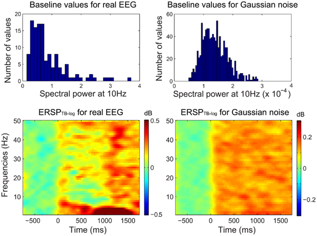
Figure 2. Single-trial baseline correction. Top row, distribution of mean single-trial baseline power values at 10 Hz for real EEG data (electrode Iz of subject “CLM” – see Materials and Methods) and for 1000 simulated trials of normalized Gaussian noise with the same time limits. Bottom row, ERSPTB − log with single-trial baseline correction tends to produce large positively biased event-related post-stimulus spectral perturbations for both the real EEG data and the artificial Gaussian noise.

Figure 3. Comparison of different baseline approaches. This figure shows spectral power at 5.8 Hz in single-trials using the classical pre-stimulus baseline ERSPz method (A), the single-trial pre-stimulus baseline ERSPTB − z method (B), and the single-trial full-epoch length correction ERSPFull TB − z method (C). The thick black line represents the average of all trials.
Figure 3 shows the apparent superiority of full-epoch length single-trial correction. For the classical baseline methods, outliers with large power values are clearly visible (Figure 3A). The middle panel (Figure 3B) shows the single-trial pre-stimulus baseline approach where data is well normalized in the baseline period. However in the post-stimulus period positive outliers are clearly visible and bias the average spectral estimate toward positive values. This is the same effect we were observing in the bottom row of Figure 2. In the last panel (Figure 3C), we use the single-trials full-epoch length correction method (see Materials and Methods), and observe that all single-trial corrected spectral estimates are within the same range of z-score values. In the rest of this manuscript, we focus on comparing classical ERSP methods versus ERSP methods based on single-trial full-epoch length correction methods.
We then compared the performance of classical ERSP methods versus single-trial full-epoch length correction methods on artificial data using the baseline permutation statistical methods (Figure 4). Figure 4A shows results for ERSPlog and ERSPFull TB − log. We chose these two ERSP methods because they exhibited the best visual contrast (Figure 6). However, using other ERSP methods return similar results. We can clearly see that TP are less sensitive to noisy trials for the single-trial method (ERSPFull TB − log) and that FN increase at a slower rate when noisy trials are added. The rate of FP is globally higher for the single-trial-based correction method than for the classical one, except when the percentage of noisy trials is lower than 8%. The bootstrap random polarity inversion method for significant testing returned qualitatively similar results.
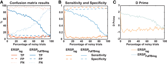
Figure 4. Confusion matrix, sensitivity, specificity, and d′ results of the ERSP classical method and the ERSP using single-trial correction. (A) True Positives (TP), False Positives (FP) and False Negatives (FN) significant results for the ERSPlog and ERSPFull TB − log. The single-trial-based method (ERSPFull TB − log) clearly outperforms the classical method (ERSPlog). (B) Sensitivity and specificity of the two methods. (C) d′ results for the two methods. Significance of ERSP results is computed using baseline permutation statistical method.
Figure 4C shows d′ values for the ERSPlog and ERSPFull TB − log methods. d′ quickly drops to 0 for the classical baseline method when as little as 2% of noisy trials are introduced, whereas the d′ for our single-trial correction method remains above 1.5 with up to 60% of noisy trials.
Table 1 indicates the specificity and sensitivity of the classical baseline correction and single-trial correction ERSPz and ERSP%/ERSPlog methods for the two types of statistical inference methods when 8.6% of trials are noisy. Significance levels between classical correction and single-trial correction methods are computed using a bootstrap procedure as described in Section “Baseline Permutation.” Irrespective of the ERSP method used, sensitivity is significantly higher by 70–80% for single-trial correction methods compared to classical correction methods for both baseline permutation statistical method and bootstrap random polarity inversion. Specificity is 2–3% higher for classical correction methods compared to single-trial correction methods although the difference is not always significant.

Table 1. Sensitivity and specificity of the classical baseline correction and single-trial correction ERSPz and ERSP%/ERSPlog methods for the two types of statistical methods when 8.6% of trials are noisy.
It may be argued that low sensitivity to noisy trials of the classical ERSP method depends on the level of the noise introduced. We thus used the same two ERSP methods on noisy trials with different amplitudes of noise. As described in the Section “Materials and Methods,” noisy trials are obtained by introducing Gaussian noise with a SD equal to the SD of the EEG multiplied by a coefficient. We used different coefficient values ranging from 1 to 5. For each coefficient value, 10 iterations were computed and the mean TP, FP, FN were calculated. Results are presented on Figure 5, which shows that for all values of coefficient greater than 1, the ERSP method using single-trial correction clearly outperforms the classical ERSP method with a higher TP rate of significant values and a comparable rate of FN responses. This performance improves as the coefficient increases.
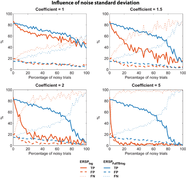
Figure 5. Confusion matrix of the ERSP classical method and the ERSP using single-trial correction for different amplitude of noise. The single-trial-based method (ERSPFull TB − log) clearly outperforms the classical method (ERSPlog) with a higher rate of True Positive significant values and a comparable rate of False Negative significant values.
Figure 6 illustrates the different ERSP approaches described in the Section “Materials and Methods” computed on one subject (see Materials and Methods): it shows ERSPs for both the classical baseline solutions (top row) and the single-trial full-epoch length corrections followed by classical baseline correction (bottom row). All methods show similar ERSP images with interesting nuances. Region 1 circled in Figure 6 shows a significant feature at high frequency that appears only when classical baseline correction methods are used. Since it is not present for the single-trial baseline correction, this region most likely represents activity from a few noisy data trials. After visual inspection of the raw data, 6 of the 126 data trials proved to contain high frequency noise. Upon removal of these data trials, region 1 is not any more significant and visible in classical method results. In addition, region 1 did not prove to be significant in any of the other 13 subjects of the same study. Region 2 shows a 500% power increase relative to baseline for the ERSP% method. The region is slightly smaller for the ERSP methods based on single-trial correction than for the classical ERSP methods. We tested the hypothesis that single-trial methods were more sensitive to noise by replacing good trials by noisy ones as described in Section “Procedure to Model Noisy Trials and Assess Robustness of ERSP Model” and computed the ERSPlog and ERSPFull TB − log for every number of noisy trials introduced in the signal. We observed that Region 2 was still significant and had the same extent for both classical and single-trial-based ERSP methods when 80% of noisy trials was introduced. Region 3 indicates a post-stimulus power decrease centered at about 13 Hz and spanning over the 10 to 15-Hz frequency band for the ERSPz method. For the ERSP% and the ERSPlog methods, a similar power decrease spans over the 6 to 15-Hz frequency band and is strongest at 6 Hz. This suggests that the variance across trials at 13 Hz is small compared to lower frequencies, which would explain why the power decrease at this frequency is larger in the ERSPz method than in the ERSP% and the ERSPlog methods. For all single-trial correction solutions, one additional significant region appears (region 4). This region corresponds to an early post-stimulus power increase in the 5 to 7-Hz frequency band. Note that the positive peak in the last panel of Figure 3 at about 200 ms corresponds to region 4 in Figure 6. To test if significance in this region was driven by noise, we applied a band-pass filter to single-trials between 5 and 7 Hz and showed that the filtered signal exceeded the SE of the average signal in the 200 to 400-ms time region. The presence of this additional region, although anecdotal, argues in favor of using single-trial baseline methods, which renders visible finer grained spectral changes. Note that the subject selected for Figure 6 was chosen for didactic purposes. When spectral activity is more homogenous across trials, the six types of ERSP are more similar.
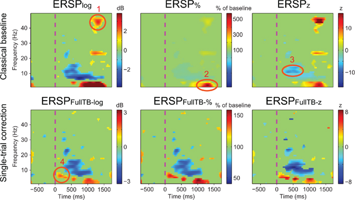
Figure 6. Results of different ERSP methods applied to channel Iz of subject “CLM” (see Materials and Methods). Images are masked for significance at p = 0.05 using the baseline permutation statistical method (see Materials and Methods) after correction for multiple comparisons using the FDR procedure. The top row shows results from classical baseline ERSP methods. The bottom row shows ERSP using full-epoch length single-trial correction. Circled regions of interest are discussed in the text.
In Figure 6, the extent of significant regions is different for the various ERSP approaches. We attempted to determine if regions of significance differed across ERSP methods. We performed ERSP decomposition for each of the 14 subjects of an animal/non-animal categorization study (see Materials and Methods), computed the percentage of significant pixels in the ERSP image, and applied a paired 2-way ANOVA on the mean percentage of significant pixels using two factors ERSP type (% or z-score) and baseline correction method (classical versus single-trial). Only the ERSP%, ERSPz, ERSPFull TB − % and ERSPFull TB − z methods were considered since the ERSPlog and ERSPFull TB − log methods are mere log-transformation of the ERSP% and ERSPFull TB − % methods which do not modify the number of significant pixels. We also tried two methods for assessing significance: baseline permutation and bootstrap random polarity inversion (see Materials and Methods).
Table 2 summarizes the mean over 14 subjects of the number of significant pixels for different ERSP methods. For the baseline permutation statistical method, the percentage of significant pixels was higher for the ERSP classical baseline methods than for the ERSP single-trial correction methods [F(1,13) = 12.504, p = 0.004]. We also observed an effect of the ERSP method [F(1,13) = 20.681, p < 0.001], where the ERSPFull TB − z method returned less significant pixels than the ERSPFull TB − % method. For the bootstrap random polarity inversion statistical method, we also observed a significant effect of the baseline correction method [F(1,13) = 5.132, p = 0.04] but in the opposite direction, the percentage of significant pixels being higher for single-trial correction methods. Bootstrap random polarity inversion statistics returned significant effect for ERSP methods in the same direction as the baseline permutation statistics [F(1,13) = 8.243, p = 0.01], where the ERSPFull TB − z method returned less significant pixels than the ERSPFull TB − % method. In sum, ERSP using baseline normalization tends to return less significant pixels than ERSP using percentages of baseline. Classical baseline and single-trial correction methods also differed significantly although the method returning more significant pixel was contingent on the statistical method used to assess significance.

Table 2. Mean percentage of significant time–frequency points (pixels) for different ERSP methods for electrode Iz.
In Figure 7, we test the hypothesis that full-epoch length single-trial baseline approaches are less sensitive to outlier trials in real EEG. To test this hypothesis, we first added noisy trials to real EEG (see Materials and Methods) and estimated the number of significant time–frequency points (pixels) for different ERSP time–frequency decomposition. We also used two independent methods to estimate significance: either the baseline permutation method or the bootstrap random polarity inversion method (see Materials and Methods). Figure 7 shows a comparison of classical baseline correction and single-trial correction for z-score ERSP methods (respectively ERSPz and ERSPFull TB − z) and percentage of baseline ERSP methods (respectively ERSP% and ERSPFull TB − %). It shows that if the percentage of noisy trials is greater than 2, the single-trial method gives more significant pixels than the classical method, although this difference decreases monotonically as the number of trials increases. Note that the percentage of significant pixels is not a true measure of sensitivity as the ones presented in Figure 4. However, given that we do not have access to the TP pixel measure, it is not possible to compute the more rigorous measures we used for artificial data.
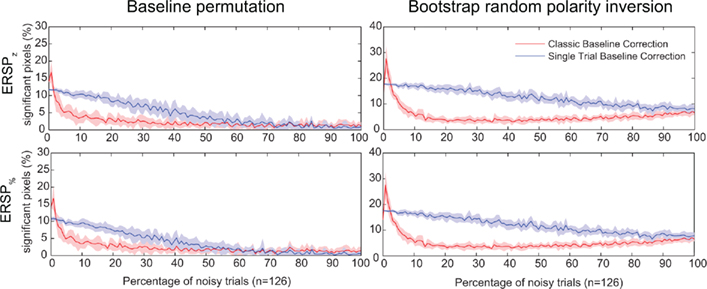
Figure 7. Percentage of significant pixels in ERSP time–frequency decompositions of real EEG data with different percentages of noisy trials. Noisy trials are added to data trials of electrode Iz from subject “CLM” (see Materials and Methods). Two different statistical methods are tested: the baseline permutation method on the left column, and the bootstrap random polarity inversion method on the right column (see Materials and Methods). The first row represents data for time–frequency decompositions computed using z-score (ERSPz and ERSPFull TB − z). The second row represents data for time–frequency decompositions computed using percentage of baseline (ERSP% and ERSPFull TB − %). Classical ERSP baseline correction methods are represented in red and single-trial correction methods are represented in blue. Shaded areas represent SD which is estimated by adding noise to different random sets (n = 10) of trials. Single-trial correction methods always outperform classical baseline methods when the number of noisy trials increases.
In order to further characterize the similarities of the ERSPs’ regions of significance, we computed the percentage of overlap between the significant regions of all pairs of ERSP methods for electrode Iz of 14 subjects (see Materials and Methods). A percentage of overlap between two ERSP methods was computed for each subject by taking the ratio between the intersection of significant regions and the union of these regions. This percentage of overlap was then averaged across subjects:

where A is the first ERSP method and B is the second one. |A ∩ B|s is the number of pixels in the intersection of significant regions computed by ERSP methods A and B for subject s; |A ∪ B|s is the number of pixels in the union of significant regions computed by ERSP methods A and B for subject s; n is the number of subjects.
Figure 8 summarizes overlaps of regions of significance between the different ERSP methods. The two procedures used to assess statistical significance produced similar results. The overlap between the ERSP classical baseline methods and the ERSP full-epoch length single-trial correction methods was only about 60–70% (Figure 8A). The overlap between classical baseline methods was about 90% and the overlap between full-epoch length single-trial correction methods was also about 90% (Figures 8B,C). Classical baseline correction methods have more overlap than single-trial correction methods for both statistical procedures [paired t-test for baseline permutation t(13) = 12.028, p < 0.001, paired t-test for bootstrap random polarity inversion, t(13) = 9.174, p < 0.001]. Note that since the statistics should be equivalent for both ERSP% and ERSPlog (respectively ERSPFull TB − % and ERSPFull TB − log), the differences observed between these two methods are due to random sampling in the bootstrap and permutation methods. Comparing Figure 8B and Figure 8C, we finally observe that the baseline permutation statistical procedure leads to higher overlap between ERSP methods than the bootstrap random polarity inversion procedure [paired t-test for classical baseline ERSP correction methods t(13) = −10.515, p < 0.001; paired t-test for single-trial correction ERSP methods, t(13) = −3.068, p < 0.001].
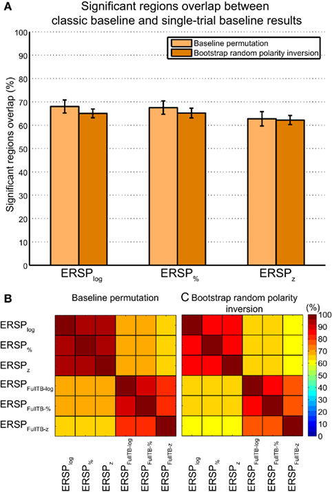
Figure 8. Average percentage of overlap of significant regions between all pairs of ERSP method for 14 subjects. The method for computing percentage of overlap is indicated in the text. (A) Bar chart of the percentage of overlap between the significant regions of ERSP using classical baseline correction and ERSP using single-trial correction. Error bars show the SE of the mean. (B) Overlap of ERSP significant regions for the baseline permutation statistical method. (C) Overlap of significant regions for the bootstrap random polarity inversion statistical method.
At each time–frequency point, Figure 9 shows the percentage of significant subjects for both the ERSP% and the ERSPFull TB − % methods as well as the overlap between them. This innovative representation allows displaying the similarities (i.e., overlap, represented in yellow) and contrast between the two ERSP methods (in red and green). We observe that even if some regions exhibit a strong overlap especially at low frequencies (in bright yellow), some other areas are more specific to one or the other of the two ERSP methods (in bright red or bright green).
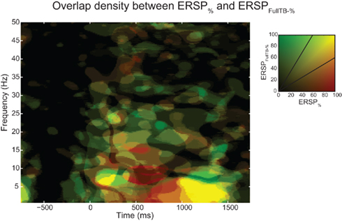
Figure 9. Density of ERSP% and ERSPFull TB − % significant pixels across subjects and their overlap. ERSPs were computed for electrode Iz of 14 subjects and significant pixels were computed using the baseline permutation method (see Materials and Methods). ERSP “density” represents the percentage of significant subject at each time–frequency point from 0 to 100% (all 14 subjects). ERSP% density of significant pixels is represented in green, ERSPFull TB − % density in red, and the overlap between ERSP% and ERSPFull TB − % densities is shown in yellow. Density is coded by color saturation level, higher densities are shown with higher saturation level.
Figure 10 shows the overlap of significant pixels across time and frequency for the ERSP% (classical baseline correction) and ERSPFull TB − % (single-trial correction) methods as well as the percentage of significant pixels for each frequency and time point. Results for the ERSPz and the ERSPFull TB − z methods are similar (not shown). Figure 10A shows that for the data analyzed here, the overlap tends to be higher at low frequencies than at higher frequencies. Figures 10B,D show the density of significant pixels and overlap across time between the two ERSP methods and indicate that for this dataset the overlap is highest in the 200 to 1000-ms time region.
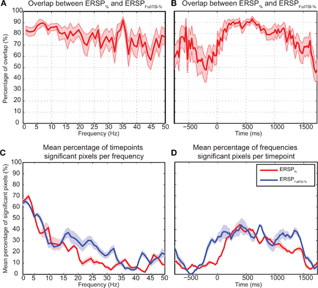
Figure 10. Number of significant pixels and overlap across time and frequency for the ERSP% and the ERSPFull TB − % methods averaged over 14 subjects. The top row shows the mean percentage of overlap between significant regions of the ERSP% (classical baseline correction) and the ERSPFull TB − % (single-trial correction) methods. (A) Average overlap between the two ERSP methods at each frequency. (B) Average overlap between the two ERSP methods at each time point. (C,D). Average percentage of significant pixels at each frequency (C) and at each time point (D). For the four curves, significant regions where computed using the bootstrap random polarity inversion method. Shaded areas show the SE of the mean.
Figure 11 focuses on the baseline time region for the two statistical methods used to compute significance and for different ERSP methods. It shows that significance during the baseline is lowest for the ERSPz and the ERSPFull TB − z methods using the baseline permutation statistical method. This argues in favor of using these ERSP methods and the baseline permutation statistical test when it is important to minimize the number of significant values in the baseline period.
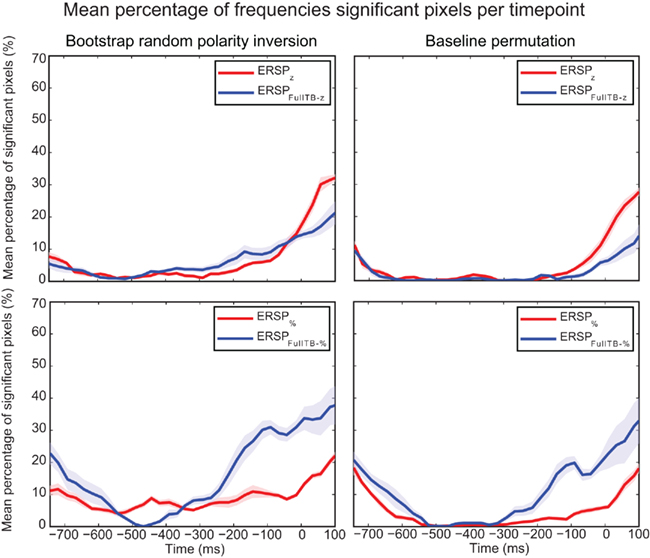
Figure 11. Mean percentage of significant pixels during the baseline period for ERSP z, ERSPFull TB − z, ERSP%, and ERSPFull TB − % using the two statistical methods. ERSPs were all computed on electrode Iz and averaged over 14 subjects. The bootstrap random polarity inversion statistical method is shown on the left column and the baseline permutation statistical method is shown on the right column. Two different ERSP methods are compared: ERSPz displayed in the upper row, and ERSP% displayed in the lower row. Classical baseline correction methods are represented in red and single-trial correction methods are represented in blue. Shaded areas represent SE of the mean.
Discussion
We have presented different ERSP methods, three based on classical baseline correction methods and three implementing single-trial correction methods. We showed the superiority of the single-trial correction methods on both artificial data and real data since these methods were less sensitive to noise compared to classical baseline correction methods. We also compared the number of significant time–frequency estimates and region of significance between all of these ERSP methods. For the data analyzed here, the overlap was strongest at low frequencies in the 200 to 1000 ms post-stimulus period. Moreover, the overlap between region of significance within classical baseline correction methods and within single-trial correction methods was always above 90%. This contrasts to 60–70% of overlap between the classical and the single-trial-based baseline correction methods and argues for a fundamental difference between these two types of approaches.
For single-trial correction methods, use of the entire time interval – including pre- and post-stimulus time intervals – may appear unconventional with respect to event-related approaches. However, processing that combines pre- and post-stimulus activity is a common procedure in EEG signal processing, as for example when performing filtering. Filtering is used in most EEG software. For example, performing high-pass FIR filtering at 0.5 Hz on continuous EEG data at 128 Hz usually requires a filter order or length of about 768. The convolution window thus comprises 6 s and might contain several stimuli: post-stimulus activity may affect pre-stimulus activity (and vice-versa), and we have observed this fact experimentally. Thus, our single-trial correction procedures combining pre- and post-stimulus activity fits well with the current EEG signal processing framework.
The main difference between the classical ERSP baseline correction methods and single-trial correction methods is that the single-trial correction approach is less sensitive to the presence of noisy trials. When adding noisy trials to the data, the number of significant pixels decreased exponentially for classical baseline correction methods. However, it decreased linearly for single-trial correction methods. This result is especially important because spectral transformations may amplify small trial noises. Even though EEG data might not appear noisy, power computed by taking the square of FFT amplitude tends to skew power distribution toward high positive values as shown in Figure 2. Therefore, using ERSP measures robust to outlier trials is important and this is why we have introduced such measures here. Other ERSP measures may also be appropriate where, for example, median ERSP values could be used instead of the mean ERSP value, and this is a potential direction for future research.
We have shown that the difference in terms of region of significance between classical baseline correction and single-trial correction methods is due to the high sensitivity of ERSP classical baseline correction to single-trial noise. This result strongly argues in favor of using single-trial correction methods when computing ERSP. Of all the methods presented in this report, we recommend using the ERSPFull TB − z in conjunction with the baseline permutation statistical method for inference testing. ERSPFull TB − z combined with this statistical method is robust to trial noise and has the lowest number of FP significant time–frequency points in the baseline period. All the methods presented in this article are implemented in the “newtimef” function of the EEGLAB software.
Conflict of Interest Statement
The authors declare that the research was conducted in the absence of any commercial or financial relationships that could be construed as a potential conflict of interest.
Acknowledgments
This work was supported by a thesis fellowship from the French ministry of research and a grant from the FRM Foundation.
References
Adeli, H., Zhou, Z., and Dadmehr, N. (2003). Analysis of EEG records in an epileptic patient using wavelet transform. J. Neurosci. Methods 123, 69–87.
Asaduzzaman, K., Reaz, M. B., Mohd-Yasin, F., Sim, K. S., and Hussain, M. S. (2010). A study on discrete wavelet-based noise removal from EEG signals. Adv. Comput. Biol. 593–599.
Basar, E., and Dumermuth, G. (1982). EEG-brain dynamics: relation between EEG and brain evoked potentials. Comput. Programs Biomed. 14, 227–228.
Benjamini, Y., and Hochberg, Y. (1995). Controlling the false discovery rate: a practical and powerful approach to multiple testing. J. R. Stat. Soc. Series B Stat. Methodol. 57, 289–300.
Bertrand, O., Bohorquez, J., and Pernier, J. (1994). Time-frequency digital filtering based on an invertible wavelet transform: an application to evoked potentials. IEEE Trans. Biomed. Eng. 41, 77–88.
Bruns, A. (2004). Fourier-, Hilbert- and wavelet-based signal analysis: are they really different approaches? J. Neurosci. Methods 137, 321–332.
Clochon, P., Fontbonne, J., Lebrun, N., and Etévenon, P. (1996). A new method for quantifying EEG event-related desynchronization: amplitude envelope analysis. Electroencephalogr. Clin. Neurophysiol. 98, 126–129.
Delorme, A., and Makeig, S. (2004). EEGLAB: an open source toolbox for analysis of single-trial EEG dynamics including independent component analysis. J. Neurosci. Methods 134, 9–21.
Delorme, A., Makeig, S., Fabre-Thorpe, M., and Sejnowski, T. (2002). From single-trial EEG to brain area dynamics. Neurocomputing 44–46, 1057–1064.
Delorme, A., Rousselet, G. A., Macé, M. J-M., and Fabre-Thorpe, et M. (2004). Interaction of top-down and bottom-up processing in the fast visual analysis of natural scenes. Cognitive Brain Res. 19, 103–113.
Delorme, A., Westerfield, M., and Makeig, S. (2007). Medial prefrontal theta bursts precede rapid motor responses during visual selective attention. J. Neurosci. 27, 11949–11959.
Freeman, W. J., Rogers, L. J., Holmes, M. D., and Silbergeld, D. L. (2000). Spatial spectral analysis of human electrocorticograms including the alpha and gamma bands. J. Neurosci. Methods 95, 111–121.
Fuentemilla, L., Marco-Pallarés, J., and Grau, C. (2006). Modulation of spectral power and of phase resetting of EEG contributes differentially to the generation of auditory event-related potentials. Neuroimage 30, 909–916.
Green, D. M., and Swets, et J. A. (1974). Signal Detection Theory and Psychophysics. Oxford, UK: Robert E. Krieger.
Herrmann, C. S., Mecklinger, A., and Pfeifer, E. (1999). Gamma responses and ERPs in a visual classification task. Clin. Neurophysiol. 110, 636–642.
Kennett, S., Eimer, M., Spence, C., and Driver, J. (2011). Tactile-visual links in exogenous spatial attention under different postures: convergent evidence from psychophysics and ERPs. J. Cogn. Neurosci. 13, 462–478.
Kim, M. S., Cho, Y. C., Abibullaev, B., and Seo, H. D. (2008). Analysis of brain function and classification of sleep stage EEG using Daubechies wavelet. Sens. Mater. 20, 1–15.
Le Van Quyen, M., Foucher, J., Lachaux, J., Rodriguez, E., Lutz, A., Martinerie, J., and Varela, F. J. (2001). Comparison of Hilbert transform and wavelet methods for the analysis of neuronal synchrony. J. Neurosci. Methods 111, 83–98.
Legewie, H., Simonova, O., and Creutzfeldt, O. D. (1969). EEG changes during performance of various tasks under open-and closed-eyed conditions. Electroencephalogr. Clin. Neurophysiol. 27, 470–479.
Lemm, S., Schafer, C., and Curio, G. (2004). BCI competition 2003-data set III: probabilistic modeling of sensorimotor μ rhythms for classification of imaginary hand movements. IEEE Trans. Biomed. Eng. 51, 1077–1080.
Luck, S. J. (2005). An Introduction to the Event-Related Potential Technique. 1st Edn. Cambridge, MA: The MIT Press.
Makeig, S. (1993). Auditory event-related dynamics of the EEG spectrum and effects of exposure to tones. Electroencephalogr. Clin. Neurophysiol. 86, 283–293.
Makeig, S., Debener, S., Onton, J., and Delorme, A. (2004). Mining event-related brain dynamics. Trends Cogn. Sci. (Regul. Ed.) 8, 204–210.
Makeig, S., Westerfield, M., Jung, T. P., Enghoff, S., Townsend, J., Courchesne, E., and Sejnowski, T. J. (2002). Dynamic brain sources of visual evoked responses. Science 295, 690.
Meltzer, J. A., Zaveri, H. P., Goncharova, I. I., Distasio, M. M., Papademetris, X., Spencer, S. S., Spencer, D. D., and Constable, R. T. (2008). Effects of working memory load on oscillatory power in human intracranial EEG. Cereb. Cortex 18, 1843–1855.
Mitra, P. P., and Pesaran, B. (1999). Analysis of dynamic brain imaging data. Biophys. J. 76, 691–708.
Nunez, P. L., and Srinivasan, R. (2006). Electric Fields of the Brain: The Neurophysics of EEG. New York: Oxford University Press.
Pfurtscheller, G. (1992). Event-related synchronization (ERS): an electrophysiological correlate of cortical areas at rest. Electroencephalogr. Clin. Neurophysiol. 83, 62–69.
Pfurtscheller, G., and Aranibar, A. (1977). Event-related cortical desynchronization detected by power measurements of scalp EEG. Electroencephalogr. Clin. Neurophysiol. 42, 817–826.
Schiff, S. J., Aldroubi, A., Unser, M., and Sato, S. (1994). Fast wavelet transformation of EEG. Electroencephalogr. Clin. Neurophysiol. 91, 442–455.
Slotnick, S. D., Moo, L. R., Kraut, M. A., Lesser, R. P., and Hart, J. Jr. (2002). Interactions between thalamic and cortical rhythms during semantic memory recall in human. Proc. Natl. Acad. Sci. 99, 6440–6443.
Tallon-Baudry, C., Bertrand, O., Delpuech, C., and Pernier, J. (1996). Stimulus specificity of phase-locked and non-phase-locked 40Hz visual responses in human. J. Neurosci. 16, 4240–4249.
Tallon-Baudry, C., Bertrand, O., and Fischer, C. (2001). Oscillatory synchrony between human extrastriate areas during visual short-term memory maintenance. J. Neurosci. 21, RC177.
Tallon-Baudry, C., Bertrand, O., Wienbruch, C., Ross, B., and Pantev, C. (1997). Combined EEG and MEG recordings of visual 40 Hz responses to illusory triangles in human. Neuroreport 8, 1103.
Tallon-Baudry, C., Kreiter, A., and Bertrand, O. (1999). Sustained and transient oscillatory responses in the gamma and beta bands in a visual short-term memory task in humans. Vis. Neurosci. 16, 449–459.
Keywords: EEG, ERP, ERS, ERSP, single-trial, baseline, additive model, multiplicative gain model
Citation: Grandchamp R and Delorme A (2011) Single-trial normalization for event-related spectral decomposition reduces sensitivity to noisy trials. Front. Psychology 2:236. doi: 10.3389/fpsyg.2011.00236
Received: 10 March 2011;
Accepted: 30 August 2011;
Published online: 30 September 2011.
Edited by:
Peter Neri, University of Aberdeen, UKReviewed by:
Giandomenico Iannetti, University of Oxford, UKThomas Charles Ferree, NeuroMetrix, Inc., USA
Copyright: © 2011 Grandchamp and Delorme. This is an open-access article subject to a non-exclusive license between the authors and Frontiers Media SA, which permits use, distribution and reproduction in other forums, provided the original authors and source are credited and other Frontiers conditions are complied with.
*Correspondence: Romain Grandchamp, Centre de Recherche Cerveau et Cognition, UMR5549, CNRS, Pavillon Baudot CHU Purpan, BP 25202, 31052 Toulouse Cedex, France. e-mail:cm9tYWluLmdyYW5kY2hhbXBAY2VyY28udXBzLXRsc2UuZnI=

