Abstract
While multicollinearity may increase the difficulty of interpreting multiple regression (MR) results, it should not cause undue problems for the knowledgeable researcher. In the current paper, we argue that rather than using one technique to investigate regression results, researchers should consider multiple indices to understand the contributions that predictors make not only to a regression model, but to each other as well. Some of the techniques to interpret MR effects include, but are not limited to, correlation coefficients, beta weights, structure coefficients, all possible subsets regression, commonality coefficients, dominance weights, and relative importance weights. This article will review a set of techniques to interpret MR effects, identify the elements of the data on which the methods focus, and identify statistical software to support such analyses.
Multiple regression (MR) is used to analyze the variability of a dependent or criterion variable using information provided by independent or predictor variables (Pedhazur, 1997). It is an important component of the general linear model (Zientek and Thompson, 2009). In fact, MR subsumes many of the quantitative methods that are commonly taught in education (Henson et al., 2010) and psychology doctoral programs (Aiken et al., 2008) and published in teacher education research (Zientek et al., 2008). One often cited assumption for conducting MR is minimal correlation among predictor variables (cf. Stevens, 2009). As Thompson (2006) explained, “Collinearity (or multicollinearity) refers to the extent to which the predictor variables have non-zero correlations with each other” (p. 234). In practice, however, predictor variables are often correlated with one another (i.e., multicollinear), which may result in combined prediction of the dependent variable.
Multicollinearity can lead to increasing complexity in the research results, thereby posing difficulty for researcher interpretation. This complexity, and thus the common admonition to avoid multicollinearity, results because the combined prediction of the dependent variable can yield regression weights that are poor reflections of variable relationships. Nimon et al. (2010) noted that correlated predictor variables can “complicate result interpretation… a fact that has led many to bemoan the presence of multicollinearity among observed variables” (p. 707). Indeed, Stevens (2009) suggested “Multicollinearity poses a real problem for the researcher using multiple regression” (p. 74).
Nevertheless, Henson (2002) observed that multicollinearity should not be seen as a problem if additional analytic information is considered:
The bottom line is that multicollinearity is not a problem in multiple regression, and therefore not in any other [general linear model] analysis, if the researcher invokes structure coefficients in addition to standardized weights. In fact, in some multivariate analyses, multicollinearity is actually encouraged, say, for example, when multi-operationalizing a dependent variable with several similar measures. (p. 13)
Although multicollinearity is not a direct statistical assumption of MR (cf. Osborne and Waters, 2002), it complicates interpretation as a function of its influence on the magnitude of regression weights and the potential inflation of their standard error (SE), thereby negatively influencing the statistical significance tests of these coefficients. Unfortunately, many researchers rely heavily on standardized (beta, β) or unstandardized (slope) regression weights when interpreting MR results (Courville and Thompson, 2001; Zientek and Thompson, 2009). In the presence of multicollinear data, focusing solely on regression weights yields at best limited information and, in some cases, erroneous interpretation. However, it is not uncommon to see authors argue for the importance of predictor variables to a regression model based on the results of null hypothesis statistical significance tests of these regression weights without consideration of the multiple complex relationships between predictors and predictors with their outcome.
Purpose
The purpose of the present article is to discuss and demonstrate several methods that allow researchers to fully interpret and understand the contributions that predictors play in forming regression effects, even when confronted with collinear relationships among the predictors. When faced with multicollinearity in MR (or other general linear model analyses), researchers should be aware of and judiciously employ various techniques available for interpretation. These methods, when used correctly, allow researchers to reach better and more comprehensive understandings of their data than would be attained if only regression weights were considered. The methods examined here include inspection of zero-order correlation coefficients, β weights, structure coefficients, commonality coefficients, all possible subsets regression, dominance weights, and relative importance weights (RIW). Taken together, the various methods will highlight the complex relationships between predictors themselves, as well as between predictors and the dependent variables. Analysis from these different standpoints allows the researcher to fully investigate regression results and lessen the impact of multicollinearity. We also concretely demonstrate each method using data from a heuristic example and provide reference information or direct syntax commands from a variety of statistical software packages to help make the methods accessible to readers.
In some cases multicollinearity may be desirable and part of a well-specified model, such as when multi-operationalizing a construct with several similar instruments. In other cases, particularly with poorly specified models, multicollinearity may be so high that there is unnecessary redundancy among predictors, such as when including both subscale and total scale variables as predictors in the same regression. When unnecessary redundancy is present, researchers may reasonably consider deletion of one or more predictors to reduce collinearity. When predictors are related and theoretically meaningful as part of the analysis, the current methods can help researchers parse the roles related predictors play in predicting the dependent variable. Ultimately, however, the degree of collinearity is a judgement call by the researcher, but these methods allow researchers a broader picture of its impact.
Predictor Interpretation Tools
Correlation coefficients
One method to evaluate a predictor’s contribution to the regression model is the use of correlation coefficients such as Pearson r, which is the zero-order bivariate linear relationship between an independent and dependent variable. Correlation coefficients are sometimes used as validity coefficients in the context of construct measurement relationships (Nunnally and Bernstein, 1994). One advantage of r is that it is the fundamental metric common to all types of correlational analyses in the general linear model (Henson, 2002; Thompson, 2006; Zientek and Thompson, 2009). For interpretation purposes, Pearson r is often squared (r2) to calculate a variance-accounted-for effect size.
Although widely used and reported, r is somewhat limited in its utility for explaining MR relationships in the presence of multicollinearity. Because r is a zero-order bivariate correlation, it does not take into account any of the MR variable relationships except that between a single predictor and the criterion variable. As such, r is an inappropriate statistic for describing regression results as it does not consider the complicated relationships between predictors themselves and predictors and criterion (Pedhazur, 1997; Thompson, 2006). In addition, Pearson r is highly sample specific, meaning that r might change across individual studies even when the population-based relationship between the predictor and criterion variables remains constant (Pedhazur, 1997).
Only in the hypothetical (and unrealistic) situation when the predictors are perfectly uncorrelated is r a reasonable representation of predictor contribution to the regression effect. This is because the overall R2 is simply the sum of the squared correlations between each predictor (X) and the outcome (Y):
This equation works only because the predictors explain different and unique portions of the criterion variable variance. When predictors are correlated and explain some of the same variance of the criterion, the sum of the squared correlations would be greater than 1.00, because r does not consider this multicollinearity.
Beta weights
One answer to the issue of predictors explaining some of the same variance of the criterion is standardized regression (β) weights. Betas are regression weights that are applied to standardized (z) predictor variable scores in the linear regression equation, and they are commonly used for interpreting predictor contribution to the regression effect (Courville and Thompson, 2001). Their utility lies squarely with their function in the standardized regression equation, which speaks to how much credit each predictor variable is receiving in the equation for predicting the dependent variable, while holding all other independent variables constant. As such, a β weight coefficient informs us as to how much change (in standardized metric) in the criterion variable we might expect with a one-unit change (in standardized metric) in the predictor variable, again holding all other predictor variables constant (Pedhazur, 1997). This interpretation of a β weight suggests that its computation must simultaneously take into account the predictor variable’s relationship with the criterion as well as the predictor variable’s relationships with all other predictors.
When predictors are correlated, the sum of the squared bivariate correlations no longer yields the R2 effect size. Instead, βs can be used to adjust the level of correlation credit a predictor gets in creating the effect:
This equation highlights the fact that β weights are not direct measures of relationship between predictors and outcomes. Instead, they simply reflect how much credit is being given to predictors in the regression equation in a particular context (Courville and Thompson, 2001). The accuracy of β weights are theoretically dependent upon having a perfectly specified model, since adding or removing predictor variables will inevitably change β values. The problem is that the true model is rarely, if ever, known (Pedhazur, 1997).
Sole interpretation of β weights is troublesome for several reasons. To begin, because they must account for all relationships among all of the variables, β weights are heavily affected by the variances and covariances of the variables in question (Thompson, 2006). This sensitivity to covariance (i.e., multicollinear) relationships can result in very sample-specific weights which can dramatically change with slight changes in covariance relationships in future samples, thereby decreasing generalizability. For example, β weights can even change in sign as new variables are added or as old variables are deleted (Darlington, 1968).
When predictors are multicollinear, variance in the criterion that can be explained by multiple predictors is often not equally divided among the predictors. A predictor might have a large correlation with the outcome variable, but might have a near-zero β weight because another predictor is receiving the credit for the variance explained (Courville and Thompson, 2001). As such, β weights are context-specific to a given specified model. Due to the limitation of these standardized coefficients, some researchers have argued for the interpretation of structure coefficients in addition to β weights (e.g., Thompson and Borrello, 1985; Henson, 2002; Thompson, 2006).
Structure coefficients
Like correlation coefficients, structure coefficients are also simply bivariate Pearson rs, but they are not zero-order correlations between two observed variables. Instead, a structure coefficient is a correlation between an observed predictor variable and the predicted criterion scores, often called “Yhat” scores (Henson, 2002; Thompson, 2006). These scores are the predicted estimate of the outcome variable based on the synthesis of all the predictors in regression equation; they are also the primary focus of the analysis. The variance of these predicted scores represents the portion of the total variance of the criterion scores that can be explained by the predictors. Because a structure coefficient represents a correlation between a predictor and the scores, a squared structure coefficient informs us as to how much variance the predictor can explain of the R2 effect observed (not of the total dependent variable), and therefore provide a sense of how much each predictor could contribute to the explanation of the entire model (Thompson, 2006).
Structure coefficients add to the information provided by β weights. Betas inform us as to the credit given to a predictor in the regression equation, while structure coefficients inform us as to the bivariate relationship between a predictor and the effect observed without the influence of the other predictors in the model. As such, structure coefficients are useful in the presence of multicollinearity. If the predictors are perfectly uncorrelated, the sum of all squared structure coefficients will equal 1.00 because each predictor will explain its own portion of the total effect (R2). When there is shared explained variance of the outcome, this sum will necessarily be larger than 1.00. Structure coefficients also allow us to recognize the presence of suppressor predictor variables, such as when a predictor has a large β weight but a disproportionately small structure coefficient that is close to zero (Courville and Thompson, 2001; Thompson, 2006; Nimon et al., 2010).
All possible subsets regression
All possible subsets regression helps researchers interpret regression effects by seeking a smaller or simpler solution that still has a comparable R2 effect size. All possible subsets regression might be referred to by an array of synonymous names in the literature, including regression weights for submodels (Braun and Oswald, 2011), all possible regressions (Pedhazur, 1997), regression by leaps and bounds (Pedhazur, 1997), and all possible combination solution in regression (Madden and Bottenberg, 1963).
The concept of all possible subsets regression is a relatively straightforward approach to explore for a regression equation until the best combination of predictors is used in a single equation (Pedhazur, 1997). The exploration consists of examining the variance explained by each predictor individually and then in all possible combinations up to the complete set of predictors. The best subset, or model, is selected based on judgments about the largest R2 with the fewest number of variables relative to the full model R2 with all predictors. All possible subsets regression is the skeleton for commonality and dominance analysis (DA) to be discussed later.
In many ways, the focus of this approach is on the total effect rather than the particular contribution of variables that make up that effect, and therefore the concept of multicollinearity is less directly relevant here. Of course, if variables are redundant in the variance they can explain, it may be possible to yield a similar effect size with a smaller set of variables. A key strength of all possible subsets regression is that no combination or subset of predictors is left unexplored.
This strength, however, might also be considered the biggest weakness, as the number of subsets requiring exploration is exponential and can be found with 2k − 1, where k represents the number of predictors. Interpretation might become untenable as the number of predictor variables increases. Further, results from an all possible subset model should be interpreted cautiously, and only in an exploratory sense. Most importantly, researchers must be aware that the model with the highest R2 might have achieved such by chance (Nunnally and Bernstein, 1994).
Commonality analysis
Multicollinearity is explicitly addressed with regression commonality analysis (CA). CA provides separate measures of unique variance explained for each predictor in addition to measures of shared variance for all combinations of predictors (Pedhazur, 1997). This method allows a predictor’s contribution to be related to other predictor variables in the model, providing a clear picture of the predictor’s role in the explanation by itself, as well as with the other predictors (Rowell, 1991, 1996; Thompson, 2006; Zientek and Thompson, 2006). The method yields all of the uniquely and commonly explained parts of the criterion variable which always sum to R2. Because CA identifies the unique contribution that each predictor and all possible combinations of predictors make to the regression effect, it is particularly helpful when suppression or multicollinearity is present (Nimon, 2010; Zientek and Thompson, 2010; Nimon and Reio, 2011). It is important to note, however, that commonality coefficients (like other MR indices) can change as variables are added or deleted from the model because of fluctuations in multicollinear relationships. Further, they cannot overcome model misspecification (Pedhazur, 1997; Schneider, 2008).
Dominance analysis
Dominance analysis was first introduced by Budescu (1993) and yields weights that can be used to determine dominance, which is a qualitative relationship defined by one predictor variable dominating another in terms of variance explained based upon pairwise variable sets (Budescu, 1993; Azen and Budescu, 2003). Because dominance is roughly determined based on which predictors explain the most variance, even when other predictors explain some of the same variance, it tends to de-emphasize redundant predictors when multicollinearity is present. DA calculates weights on three levels (complete, conditional, and general), within a given number of predictors (Azen and Budescu, 2003).
Dominance levels are hierarchical, with complete dominance as the highest level. Complete dominance is inherently both conditional and generally dominant. The reverse, however, is not necessarily true; a generally dominant variable is not necessarily conditionally or completely dominant. Complete dominance occurs when a predictor has a greater dominance weight, or average additional R2, in all possible pairwise (and combination) comparisons. However, complete dominance does not typically occur in real data. Because predictor dominance can present itself in more practical intensities, two lower levels of dominance were introduced (Azen and Budescu, 2003).
The middle level of dominance, referred as conditional dominance, is determined by examining the additional contribution to R2 within specific number of predictors (k). A predictor might conditionally dominate for k = 2 predictors, but not necessarily k = 0 or 1. The conditional dominance weight is calculated by taking the average R2 contribution by a variable for a specific k. Once the conditional dominance weights are calculated, the researcher can interpret the averages in pairwise fashion across all k predictors.
The last and lowest level of dominance is general. General dominance averages the overall additional contributions of R2. In simple terms, the average weights from each k group (k = 0, 1, 2) for each predictor (X1, X2, and X3) are averaged for the entire model. General dominance is relaxed compared to the complete and conditional dominance weights to alleviate the number of undetermined dominance in data analysis (Azen and Budescu, 2003). General dominance weights provide similar results as RIWs, proposed by Lindeman et al. (1980) and Johnson (2000, 2004). RIWs and DA are deemed the superior MR interpretation techniques by some (Budescu and Azen, 2004), almost always producing consistent results between methods (Lorenzo-Seva et al., 2010). Finally, an important point to emphasize is that the sum of the general dominance weights will equal the multiple R2 of the model.
Several strengths are noteworthy with a full DA. First, dominance weights provide information about the contribution of predictor variables across all possible subsets of the model. In addition, because comparisons can be made across all pairwise comparisons in the model, DA is sensitive to patterns that might be present in the data. Finally, complete DA can be a useful tool for detection and interpretation of suppression cases (Azen and Budescu, 2003).
Some weaknesses and limitations of DA exist, although some of these weaknesses are not specific to DA. DA is not appropriate in path analyses or to test a specific hierarchical model (Azen and Budescu, 2003). DA is also not appropriate for mediation and indirect effect models. Finally, as is true with all other methods of variable interpretation, model misspecification will lead to erroneous interpretation of predictor dominance (Budescu, 1993). Calculations are also thought by some to be laborious as the number of predictors increases (Johnson, 2000).
Relative importance weights
Relative importance weights can also be useful in the presence of multicollinearity, although like DA, these weights tend to focus on attributing general credit to primary predictors rather than detailing the various parts of the dependent variable that are explained. More specifically, RIWs are the proportionate contribution from each predictor to R2, after correcting for the effects of the intercorrelations among predictors (Lorenzo-Seva et al., 2010). This method is recommended when the researcher is examining the relative contribution each predictor variable makes to the dependent variable rather than examining predictor ranking (Johnson, 2000, 2004) or having concern with specific unique and commonly explained portions of the outcome, as with CA. RIWs range between 0 and 1, and their sum equals R2 (Lorenzo-Seva et al., 2010). The weights most always match the values given by general dominance weights, despite being derived in a different fashion.
Relative importance weights are computed in four major steps (see full detail in Johnson, 2000; Lorenzo-Seva et al., 2010). Step one transforms the original predictors (X) into orthogonal variables (Z) to achieve the highest similarity of prediction compared to the original predictors but with the condition that the transformed predictors must be uncorrelated. This initial step is an attempt to simplify prediction of the criterion by removing multicollinearity. Step two involves regressing the dependent variable (Y) onto the orthogonalized predictors (Z), which yields the standardized weights for each Z. Because the Zs are uncorrelated, these β weights will equal the bivariate correlations between Y and Z, thus making equations (1) and (2) above the same. In a three predictor model, for example, the result would be a 3 × 1 weight matrix (β) which is equal to the correlation matrix between Y and the Zs. Step three correlates the orthogonal predictors (Z) with the original predictors (X) yielding a 3 × 3 matrix (R) in a three predictor model. Finally, step four calculates the RIWs (ε) by multiplying the squared ZX correlations (R) with the squaredYZ weights (β).
Relative importance weights are perhaps more efficiently computed as compared to computation of DA weights which requires all possible subsets regressions as building blocks (Johnson, 2004; Lorenzo-Seva et al., 2010). RIWs and DA also yield almost identical solutions, despite different definitions (Johnson, 2000; Lorenzo-Seva et al., 2010). However, these weights do not allow for easy identification of suppression in predictor variables.
Heuristic Demonstration
When multicollinearity is present among predictors, the above methods can help illuminate variable relationships and inform researcher interpretation. To make their use more accessible to applied researchers, the following section demonstrates these methods using a heuristic example based on the classic suppression correlation matrix from Azen and Budescu (2003), presented in Table 1. Table 2 lists statistical software or secondary syntax programs available to run the analyses across several commonly used of software programs – blank spaces in the table reflect an absence of a solution for that particular analysis and solution, and should be seen as an opportunity for future development. Sections “Excel For All Available Analyses, R Code For All Available Analyses, SAS Code For All Available Analyses, and SPSS Code For All Analyses” provide instructions and syntax commands to run various analyses in Excel, R, SAS, and SPSS, respectively. In most cases, the analyses can be run after simply inputting the correlation matrix from Table 1 (n = 200 cases was used here). For SPSS (see SPSS Code For All Analyses), some analyses require the generation of data (n = 200) using the syntax provided in the first part of the appendix (International Business Machines Corp, 2010). Once the data file is created, the generic variable labels (e.g., var1) can be changed to match the labels for the correlation matrix (i.e., Y, X1, X2, and X3).
Table 1
| Y | X1 | X2 | X3 | |
|---|---|---|---|---|
| Y | 1.000 | |||
| X1 | 0.500 | 1.000 | ||
| X2 | 0.000 | 0.300 | 1.000 | |
| X3 | 0.250 | 0.250 | 0.250 | 1.000 |
Correlation matrix for classical suppression example (Azen and Budescu, 2003).
Reprinted with permission from Azen and Budescu (2003). Copyright 2003 by Psychological Methods.
Table 2
| Program | Beta weights | Structure coefficients | All possible subsets | Commonality analysisc | Relative weights | Dominance analysis |
|---|---|---|---|---|---|---|
| Excel | Base | rs = ry.x1/R | Braun and Oswald (2011)a | Braun and Oswald (2011)a | Braun and Oswald (2011)a | |
| R | Nimon and Roberts (2009) | Nimon and Roberts (2009) | Lumley (2009) | Nimon et al. (2008) | ||
| SAS | Base | base | baseb | Tonidandel et al. (2009)d | Azen and Budescu (2003)b | |
| SPSS | Base | Lorenzo-Seva et al. (2010) | Nimon (2010) | Nimon (2010) | Lorenzo-Seva et al. (2010), Lorenzo-Seva and Ferrando (2011), LeBreton and Tonidandel (2008) |
Tools to support interpreting multiple regression.
aUp to 9 predictors, bup to 10 predictors, cA FORTRAN IV computer program to accomplish commonality analysis was developed by Morris (1976). However, the program was written for a mainframe computer and is now obsolete, dThe Tonidandel et al. (2009) SAS solution computes relative weights with a bias correction, and thus results do not mirror those in the current paper. As such, we have decided not to demonstrate the solution here. However, the macro can be downloaded online (http://www1.davidson.edu/academic/psychology/Tonidandel/TonidandelProgramsMain.htm) and provides user-friendly instructions.
All of the results are a function of regressing Y on X1, X2, and X3 via MR. Table 3 presents the summary results of this analysis, along with the various coefficients and weights examined here to facilitate interpretation.
Table 3
| Predictor | β | rs | r | R2 | Uniquea | Commona | General dominance weightsb | Relative importance weights | |
|---|---|---|---|---|---|---|---|---|---|
| X1 | 0.517 | 0.911 | 0.830 | 0.500 | 0.250 | 0.234 | 0.016 | 0.241 | 0.241 |
| X2 | −0.198 | 0.000 | 0.000 | 0.000 | 0.000 | 0.034 | −0.034 | 0.016 | 0.015 |
| X3 | 0.170 | 0.455 | 0.207 | 0.250 | 0.063 | 0.026 | 0.037 | 0.044 | 0.045 |
Multiple regression results.
R2 = 0.301. The primary predictor suggested by a method is underlined. r is correlation between predictor and outcome variable.
rs = structure coefficient = r/R. . Unique = proportion of criterion variance explained uniquely by the predictor. Common = proportion of criterion variance explained by the predictor that is also explained by one or more other predictors. Unique + Common = r2. Σ General dominance weights = Σ relative importance weights = R2. aSee Table 5 for full CA. bSee Table 6 for full DA.
Correlation coefficients
Examination of the correlations in Table 1 indicate that the current data indeed have collinear predictors (X1, X2, and X3), and therefore some of the explained variance of Y (R2 = 0.301) may be attributable to more than one predictor. Of course, the bivariate correlations tell us nothing directly about the nature of shared explained variance. Here, the correlations between Y and X1, X2, and X3 are 0.50, 0, and 0.25, respectively. The squared correlations (r2) suggest that X1 is the strongest predictor of the outcome variable, explaining 25% (r2 = 0.25) of the criterion variable variance by itself. The zero correlation between Y and X2 suggests that there is no relationship between these variables. However, as we will see through other MR indices, interpreting the regression effect based only on the examination of correlation coefficients would provide, at best, limited information about the regression model as it ignores the relationships between predictors themselves.
Beta weights
The β weights can be found in Table 3. They form the standardized regression equation which yields predicted Y scores: where all predictors are in standardized (Z) form. The squared correlation between Y and equals the overall R2 and represents the amount of variance of Y that can be explained by and therefore by the predictors collectively. The β weights in this equation speak to the amount of credit each predictor is receiving in the creation of and therefore are interpreted by many as indicators of variable importance (cf. Courville and Thompson, 2001; Zientek and Thompson, 2009).
In the current example, indicating that about 30% of the criterion variance can be explained by the predictors. The β weights reveal that X1 (β = 0.517) received more credit in the regression equation, compared to both X2 (β = −0.198) and X3 (β = 0.170). The careful reader might note that X2 received considerable credit in the regression equation predicting Y even though its correlation with Y was 0. This oxymoronic result will be explained later as we examine additional MR indices. Furthermore, these results make clear that the βs are not direct measures of relationship in this case since the β for X2 is negative even though the zero-order correlation between the X2 and Y is positive. This difference in sign is a good first indicator of the presence of multicollinear data.
Structure coefficients
The structure coefficients are given in Table 3 as rs. These are simply the Pearson correlations between and each predictor. When squared, they yield the proportion of variance in the effect (or, of the scores) that can be accounted for by the predictor alone, irrespective of collinearity with other predictors. For example, the squared structure coefficient for X1 was 0.830 which means that of the 30.1% (R2) effect, X1 can account for 83% of the explained variance by itself. A little math would show that 83% of 30.1% is 0.250, which matches the r2 in Table 3 as well. Therefore, the interpretation of a (squared) structure coefficient is in relation to the explained effect rather than to the dependent variable as a whole.
Examination of the β weights and structure coefficients in the current example suggests that X1 contributed most to the variance explained with the largest absolute value for both the β weight and structure coefficient (β = 0.517, rs = 0.911 or ). The other two predictors have somewhat comparable βs but quite dissimilar structure coefficients. Predictor X3 can explain about 21% of the obtained effect by itself (β = 0.170, rs = 0.455, ), but X2 shares no relationship with the scores (β = −0.198, rs and ).
On the surface it might seem a contradiction for X2 to explain none of the effect but still be receiving credit in the regression equation for creating the predicted scores. However, in this case X2 is serving as a suppressor variable and helping the other predictor variables do a better job of predicting the criterion even though X2 itself is unrelated to the outcome. A full discussion of suppression is beyond the scope of this article1. However, the current discussion makes apparent that the identification of suppression would be unlikely if the researcher were to only examine β weights when interpreting predictor contributions.
Because a structure coefficient speaks to the bivariate relationship between a predictor and an observed effect, it is not directly affected by multicollinearity among predictors. If two predictors explain some of the same part of the score variance, the squared structure coefficients do not arbitrarily divide this variance explained among the predictors. Therefore, if two or more predictors explain some of the same part of the criterion, the sum the squared structure coefficients for all predictors will be greater than 1.00 (Henson, 2002). In the current example, this sum is 1.037 (0.830 + 0 + 0.207), suggesting a small amount of multicollinearity. Because X2 is unrelated to Y, the multicollinearity is entirely a function of shared variance between X1 and X3.
All possible subsets regression
We can also examine how each of the predictors explain Y both uniquely and in all possible combinations of predictors. With three variables, seven subsets are possible (2k − 1 or 23 − 1). The R2 effects from each of these subsets are given in Table 4, which includes the full model effect of 30.1% for all three predictors. Predictors X1 and X2 explain roughly 27.5% of the variance in the outcome. The difference between a three predictor versus this two predictor model is a mere 2.6% (30.1−27.5), a relatively small amount of variance explained. The researcher might choose to drop X3, striving for parsimony in the regression model. A decision might also be made to drop X2 given its lack of prediction of Y independently. However, careful examination of the results speaks again to the suppression role of X2, which explains none of Y directly but helps X1 and X3 explain more than they could by themselves when X2 is added to the model. In the end, decisions about variable contributions continue to be a function of thoughtful researcher judgment and careful examination of existing theory. While all possible subsets regression is informative, this method generally lacks the level of detail provided by both βs and structure coefficients.
Table 4
| Predictor set | R2 |
|---|---|
| X1 | 0.250 |
| X2 | 0.000 |
| X3 | 0.063 |
| X1, X2 | 0.275 |
| X1, X3 | 0.267 |
| X2, X3 | 0.067 |
| X1, X2, X3 | 0.301 |
All possible subsets regression.
Predictor contribution is determined by researcher judgment. The model with the highest R2 value, but with the most ease of interpretation, is typically chosen.
Commonality analysis
Commonality analysis takes all possible subsets further and divides all of the explained variance in the criterion into unique and common (or shared) parts. Table 5 presents the commonality coefficients, which represent the proportions of variance explained in the dependent variable. The unique coefficient for X1 (0.234) indicates that X1 uniquely explains 23.4% of the variance in the dependent variable. This amount of variance is more than any other partition, representing 77.85% of the R2 effect (0.301). The unique coefficient for X3 (0.026) is the smallest of the unique effects and indicates that the regression model only improves slightly with the addition of variable X3, which is the same interpretation provided by the all possible subsets analysis. Note that X2 uniquely accounts for 11.38% of the variance in the regression effect. Again, this outcome is counterintuitive given that the correlation between X2 and Y is zero. However, as the common effects will show, X2 serves as a suppressor variable, yielding a unique effect greater than its total contribution to the regression effect and negative commonality coefficients.
Table 5
| Predictor(s) | X1 | X2 | X3 | Coefficient | Percent |
|---|---|---|---|---|---|
| X1 | 0.234 | 0.234 | 77.845 | ||
| X2 | 0.034 | 0.034 | 11.381 | ||
| X3 | 0.026 | 0.026 | 8.702 | ||
| X1, X2 | −0.030 | −0.030 | −0.030 | −10.000 | |
| X1, X3 | 0.041 | 0.041 | 0.041 | 13.453 | |
| X2, X3 | −0.010 | −0.010 | −0.010 | −3.167 | |
| X1, X2, X3 | 0.005 | 0.005 | 0.005 | 0.005 | 1.779 |
| Total | 0.250 | 0.000 | 0.063 | 0.301 | 100.000 |
Commonality coefficients.
Commonality coefficients identifying suppression underlined.
ΣXk Commonality coefficients equals r2 between predictor (k) and dependent variable.
Σ Commonality coefficients equals Multiple R2 = 30.1%. Percent = coefficient/multiple R2.
The common effects represent the proportion of criterion variable variance that can be jointly explained by two or more predictors together. At this point the issue of multicollinearity is explicitly addressed with an estimate of each part of the dependent variable that can be explained by more than one predictor. For example, X1 and X3 together explain 4.1% of the outcome, which represents 13.45% of the total effect size.
It is also important to note the presence of negative commonality coefficients, which seem anomalous given that these coefficients are supposed to represent variance explained. Negative commonality coefficients are generally indicative of suppression (cf. Capraro and Capraro, 2001). In this case, they indicate that X2 suppresses variance in X1 and X3 that is irrelevant to explaining variance in the dependent variable, making the predictive power of their unique contributions to the regression effect larger than they would be if X2 was not in the model. In fact, if X2 were not in the model, X1 and X3 would respectively only account for 20.4% (0.234−0.030) and 1.6% (0.026−0.010) of unique variance in the dependent variable. The remaining common effects indicate that, as noted above, multicollinearity between X1 and X3 accounts for 13.45% of the regression effect and that there is little variance in the dependent variable that is common across all three predictor variables. Overall, CA can help to not only identify the most parsimonious model, but also quantify the location and amount of variance explained by suppression and multicollinearity.
Dominance weights
Referring to Table 6, the conditional dominance weights for the null or k = 0 subset reflects the r2 between the predictor and the dependent variable. For the subset model where k = 2, note that the additional contribution each variable makes to R2 is equal to the unique effects identified from CA. In the case when k = 1, DA provides new information to interpreting the regression effect. For example, when X2 is added to a regression model with X1, DA shows that the change (Δ) in R2 is 0.025.
Table 6
| Subset model | Additional contribution of: | |||
|---|---|---|---|---|
| X1 | X2 | X3 | ||
| Null and k = 0 average | 0 | 0.250 | 0.000 | 0.063 |
| X1 | 0.250 | 0.025 | 0.017 | |
| X2 | 0.000 | 0.275 | 0.067 | |
| X3 | 0.063 | 0.204 | 0.004 | |
| k = 1 average | 0.240 | 0.015 | 0.044a | |
| X1, X2 | 0.275 | 0.026 | ||
| X1, X3 | 0.267 | 0.034 | ||
| X2, X3 | 0.067 | 0.234 | ||
| k = 2 average | 0.234 | 0.034 | 0.026 | |
| X1, X2, X3 | 0.301 | |||
| Overall average | 0.241 | 0.016 | 0.044 | |
Full dominance analysis (Azen and Budescu, 2003).
The DA weights are typically used to determine if variables have complete, conditional, or general dominance. When evaluating for complete dominance, all pairwise comparisons must be considered. Looking across all rows to compare the size of dominance weights, we see that X1 consistently has a larger conditional dominance weight. Because of this, it can be said that predictor X1 completely dominates the other predictors. When considering conditional dominance, however, only three rows must be considered: these are labeled null and k = 0, k = 1, and k = 2 rows. These rows provide information about which predictor dominates when there are 0, 1, and 2 additional predictors present. From this, we see that X1 conditionally dominates in all model sizes with weights of 0.250 (k = 0), 0.240 (k = 1), and 0.234 (k = 2). Finally, to evaluate for general dominance, only one row must be attended to. This is the overall average row. General dominance weights are the average conditional dominance weight (additional contribution of R2) for each variable across situations. For example, X1 generally dominates with a weight of 0.241 [i.e., (0.250 + 0.240 + 0.234)/3]. An important observation is the sum of the general dominance weights (0.241 + 0.016 + 0.044) is also equal to 0.301, which is the total model R2 for the MR analysis.
Relative importance weights
Relative importance weights were computed using the Lorenzo-Seva et al. (2010) SPSS code using the correlation matrix provided in Table 1. Based on RIW (Johnson, 2001), X1 would be considered the most important variable (RIW = 0.241), followed by X3 (RIW = 0.045) and X2 (RIW = 0.015). The RIWs offer an additional representation of the individual effect of each predictor while simultaneously considering the combination of predictors as well (Johnson, 2000). The sum of the weights (0.241 + 0.045 + 0.015 = 0.301) is equal to R2. Predictor X1 can be interpreted as the most important variable relative to other predictors (Johnson, 2001). The interpretation is consistent with a full DA, because both the individual predictor contribution with the outcome variable (rX1·Y), and the potential multicollinearity (rX1·X2 and rX1·X3) with other predictors are accounted for. While the RIWs may differ slightly compared to general dominance weights (e.g., 0.015 and 0.016, respectively, for X2), the conclusions are the consistent with those from a full DA. This method rank orders the variables with X1 as the most important, followed by X3 and X2. The suppression role of X2, however, is not identified by this method, which helps explain its rank as third in this process.
Discussion
Predictor variables are more commonly correlated than not in most practical situations, leaving researchers with the necessity to addressing such multicollinearity when they interpret MR results. Historically, views about the impact of multicollinearity on regression results have ranged from challenging to highly problematic. At the extreme, avoidance of multicollinearity is sometimes even considered a prerequisite assumption for conducting the analysis. These perspectives notwithstanding, the current article has presented a set of tools that can be employed to effectively interpret the roles various predictors have in explaining variance in a criterion variable.
To be sure, traditional reliance on standardized or unstandardized weights will often lead to poor or inaccurate interpretations when multicollinearity or suppression is present in the data. If researchers choose to rely solely on the null hypothesis statistical significance test of these weights, then the risk of interpretive error is noteworthy. This is primarily because the weights are heavily affected by multicollinearity, as are their SE which directly impact the magnitude of the corresponding p values. It is this reality that has led many to suggest great caution when predictors are correlated.
Advances in the literature and supporting software technology for their application have made the issue of multicollinearity much less critical. Although predictor correlation can certainly complicate interpretation, use of the methods discussed here allow for a much broader and more accurate understanding of the MR results regarding which predictors explain how much variance in the criterion, both uniquely and in unison with other predictors.
In data situations with a small number of predictors or very low levels of multicollinearity, the interpretation method used might not be as important as results will most often be very similar. However, when the data situation becomes more complicated (as is often the case in real-world data, or when suppression exists as exampled here), more care is needed to fully understand the nature and role of predictors.
Cause and effect, theory, and generalization
Although current methods are helpful, it is very important that researchers remain aware that MR is ultimately a correlational-based analysis, as are all analyses in the general linear model. Therefore, variable correlations should not be construed as evidence for cause and effect relationships. The ability to claim cause and effect are predominately issues of research design rather than statistical analysis.
Researchers must also consider the critical role of theory when trying to make sense of their data. Statistics are mere tools to help understand data, and the issue of predictor importance in any given model must invoke the consideration of the theoretical expectations about variable relationships. In different contexts and theories, some relationships may be deemed more or less relevant.
Finally, the pervasive impact of sampling error cannot be ignored in any analytical approach. Sampling error limits the generalizability of our findings and can cause any of the methods described here to be more unique to our particular sample than to future samples or the population of interest. We should not assume too easily that the predicted relationships we observe will necessarily appear in future studies. Replication continues to be a key hallmark of good science.
Interpretation Methods
The seven approaches discussed here can help researchers better understand their MR models, but each has its own strengths and limitations. In practice, these methods should be used to inform each other to yield a better representation of the data. Below we summarize the key utility provided by each approach.
Pearson r correlation coefficient
Pearson r is commonly employed in research. However, as illustrated in the heuristic example, r does not take into account the multicollinearity between variables and they do not allow detection of suppressor effects.
Beta weights and structure coefficients
Interpretations of both β weights and structure coefficients provide a complementary comparison of predictor contribution to the regression equation and the variance explained in the effect. Beta weights alone should not be utilized to determine the contribution predictor variables make to a model because a variable might be denied predictive credit in the presence of multicollinearity. Courville and Thompson, 2001; see also Henson, 2002) advocated for the interpretation of (a) both β weights and structure coefficients or (b) both β weights and correlation coefficients. When taken together, β and structure coefficients can illuminate the impact of multicollinearity, reflect more clearly the ability of predictors to explain variance in the criterion, and identify suppressor effects. However, they do not necessarily provide detailed information about the nature of unique and commonly explained variance, nor about the magnitude of the suppression.
All possible subsets regression
All possible subsets regression is exploratory and comes with increasing interpretive difficulty as predictors are added to the model. Nevertheless, these variance portions serve as the foundation for unique and common variance partitioning and full DA.
Commonality analysis, dominance analysis, and relative importance weights
Commonality analysis decomposes the regression effect into unique and common components and is very useful for identifying the magnitude and loci of multicollinearity and suppression. DA explores predictor contribution in a variety of situations and provides consistent conclusions with RIWs. Both general dominance and RIWs provide alternative techniques to decomposing the variance in the regression effect and have the desirable feature that there is only one coefficient per independent variable to interpret. However, the existence of suppression is not readily understood by examining general dominance weights or RIWs. Nor do the indices yield information regarding the magnitude and loci of multicollinearity.
Conclusion
The real world can be complex – and correlated. We hope the methods summarized here are useful for researchers using regression to confront this multicollinear reality. For both multicollinearity and suppression, multiple pieces of information should be consulted to understand the results. As such, these data situations should not be shunned, but simply handled with appropriate interpretive frameworks. Nevertheless, the methods are not a panacea, and require appropriate use and diligent interpretation. As correctly stated by Wilkinson and the APA Task Force on Statistical Inference (1999), “Good theories and intelligent interpretation advance a discipline more than rigid methodological orthodoxy… Statistical methods should guide and discipline our thinking but should not determine it” (p. 604).
Statements
Conflict of interest
The authors declare that the research was conducted in the absence of any commercial or financial relationships that could be construed as a potential conflict of interest.
Footnotes
1.^Suppression is apparent when a predictor has a beta weight that is disproportionately large (thus receiving predictive credit) relative to a low or near-zero structure coefficient (thus indicating no relationship with the predicted scores). For a broader discussion of suppression, see Pedhazur (1997) and Thompson (2006).
References
1
AikenL. S.WestS. G.MillsapR. E. (2008). Doctorial training in statistics, measurement, and methodology in psychology: replication and extension of Aiken, West, Sechrest, and Reno’s (1990) survey of PhD programs in North America. Am. Psychol.63, 32–50.10.1037/0003-066X.63.1.32
2
AzenR.BudescuD. V. (2003). The dominance analysis approach to comparing predictors in multiple regression. Psychol. Methods8, 129–148.10.1037/1082-989X.8.2.129
3
BraunM. T.OswaldF. L. (2011). Exploratory regression analysis: a tool for selecting models and determining predictor importance. Behav. Res. Methods43, 331–339.10.3758/s13428-010-0046-8
4
BudescuD. V. (1993). Dominance analysis: a new approach to the problem of relative importance of predictors in multiple regression. Psychol. Bull.114, 542–551.10.1037/0033-2909.114.3.542
5
BudescuD. V.AzenR. (2004). Beyond global measures of relative importance: some insights from dominance analysis. Organ. Res. Methods7, 341–350.10.1177/1094428104267049
6
CapraroR. M.CapraroM. M. (2001). Commonality analysis: understanding variance contributions to overall canonical correlation effects of attitude toward mathematics on geometry achievement. Mult. Lin. Regression Viewpoints27, 16–23.
7
CourvilleT.ThompsonB. (2001). Use of structure coefficients in published multiple regression articles: is not enough. Educ. Psychol. Meas.61, 229–248.10.1177/00131640121971211
8
DarlingtonR. B. (1968). Multiple regression in psychological research and practice. Psychol. Bull.69, 161–182.10.1037/h0025471
9
HensonR. K. (2002). The logic and interpretation of structure coefficients in multivariate general linear model analyses. Paper Presented at the Annual Meeting of the American Educational Research Association, New Orleans.
10
HensonR. K.HullD. M.WilliamsC. (2010). Methodology in our education research culture: toward a stronger collective quantitative proficiency. Educ. Res.39, 229–240.10.3102/0013189X10365102
11
International Business Machines Corp. (2010). Can SPSS Help me Generate a File of Raw Data with a Specified Correlation Structure? Available at: https://www-304.ibm.com/support/docview.wss?uid=swg21480900
12
JohnsonJ. W. (2000). A heuristic method for estimating the relative weight of predictor variables in multiple regression. Multivariate Behav. Res.35, 1–19.10.1207/S15327906MBR3501_1
13
JohnsonJ. W. (2001). “Determining the relative importance of predictors in multiple regression: practical applications of relative weights,” in Advances in Psychology Research, Vol. V, eds ColumbusF.ColumbusF. (Hauppauge, NY: Nova Science Publishers), 231–251.
14
JohnsonJ. W. (2004). Factors affecting relative weights: the influence of sampling and measurement error. Organ. Res. Methods7, 283–299.10.1177/1094428104266510
15
LeBretonJ. M.TonidandelS. (2008). Multivariate relative importance: relative weight analysis to multivariate criterion spaces. J. Appl. Psychol.93, 329–345.10.1037/0021-9010.93.2.329
16
LindemanR. H.MerendaP. F.GoldR. Z. (1980). Introduction to Bivariate and Multivariate Analysis. Glenview, IL: Scott Foresman.
17
Lorenzo-SevaU.FerrandoP. J. (2011). FIRE: an SPSS program for variable selection in multiple linear regression via the relative importance of predictors. Behav. Res. Methods43, 1–7.10.3758/s13428-010-0043-y
18
Lorenzo-SevaU.FerrandoP. J.ChicoE. (2010). Two SPSS programs for interpreting multiple regression results. Behav. Res. Methods42, 29–35.10.3758/BRM.42.1.29
19
LumleyT. (2009). Leaps: Regression Subset Selection. R Package Version 2.9. Available at: http://CRAN.R-project.org/package=leaps
20
MaddenJ. M.BottenbergR. A. (1963). Use of an all possible combination solution of certain multiple regression problems. J. Appl. Psychol.47, 365–366.10.1037/h0040365
21
MorrisJ. D. (1976). A computer program to accomplish commonality analysis. Educ. Psychol. Meas.36, 721–723.10.1177/001316447603600319
22
NimonK. (2010). Regression commonality analysis: demonstration of an SPSS solution. Mult. Lin. Regression Viewpoints36, 10–17.
23
NimonK.HensonR.GatesM. (2010). Revisiting interpretation of canonical correlation analysis: a tutorial and demonstration of canonical commonality analysis. Multivariate Behav. Res.45, 702–724.10.1080/00273171.2010.498293
24
NimonK.LewisM.KaneR.HaynesR. M. (2008). An R package to compute commonality coefficients in the multiple regression case: an introduction to the package and a practical example. Behav. Res. Methods40, 457–466.10.3758/BRM.40.2.457
25
NimonK.ReioT. (2011). Regression commonality analysis: a technique for quantitative theory building. Hum. Resour. Dev. Rev.10, 329–340.10.1177/1534484311411077
26
NimonK.RobertsJ. K. (2009). Yhat: Interpreting Regression effects. R Package Version 1.0-3. Available at: http://CRAN.R-project.org/package=yhat
27
NunnallyJ.C.BernsteinI. H. (1994). Psychometric Theory, 3rd Edn. New York: McGraw-Hill.
28
OsborneJ.WatersE. (2002). Four assumptions of multiple regression that researchers should always test. Practical Assessment, Research & Evaluation, 8(2). Available at: http://PAREonline.net/getvn.asp?v=8&n=2 [accessed December 12, 2011]
29
PedhazurE. J. (1997). Multiple Regression in Behavioral Research: Explanation and Prediction, 3rd Edn. Fort Worth, TX: Harcourt Brace.
30
RowellR. K. (1991). Partitioning predicted variance into constituent parts: how to conduct commonality analysis. Paper Presented at the Annual Meeting of the Southwest Educational Research Association, San Antonio.
31
RowellR. K. (1996). “Partitioning predicted variance into constituent parts: how to conduct commonality analysis,” in Advances in Social science Methodology, Vol. 4, ed. ThompsonB. (Greenwich, CT: JAI Press), 33–44.
32
SchneiderW. J. (2008). Playing statistical ouija board with commonality analysis: good questions, wrong assumptions. Appl. Neuropsychol.15, 44–53.10.1080/09084280801917566
33
StevensJ. P. (2009). Applied Multivariate Statistics for the Social Sciences, 4th Edn. New York: Routledge.
34
ThompsonB. (2006). Foundations of Behavioral Statistics: An Insight-Based Approach. New York: Guilford Press.
35
ThompsonB.BorrelloG. M. (1985). The importance of structure coefficients in regression research. Educ. Psychol. Meas.45, 203–209.
36
TonidandelS.LeBretonJ. M.JohnsonJ. W. (2009). Determining the statistical significance of relative weights. Psychol. Methods14, 387–399.10.1037/a0017735
37
UCLA: Academic Technology Services Statistical Consulting Group. (n.d.). Introduction to SAS. Available at: http://www.ats.ucla.edu/stat/sas
38
WilkinsonL.APA Task Force on Statistical Inference. (1999). Statistical methods in psychology journals: guidelines and explanation. Am. Psychol.54, 594–604.10.1037/0003-066X.54.8.594
39
ZientekL. R.CapraroM. M.CapraroR. M. (2008). Reporting practices in quantitative teacher education research: one look at the evidence cited in the AERA panel report. Educ. Res.37, 208–216.10.3102/0013189X08319762
40
ZientekL. R.ThompsonB. (2006). Commonality analysis: partitioning variance to facilitate better understanding of data. J. Early Interv.28, 299–307.10.1177/105381510602800405
41
ZientekL. R.ThompsonB. (2009). Matrix summaries improve research reports: secondary analyses using published literature. Educ. Res.38, 343–352.10.3102/0013189X09339056
42
ZientekL. R.ThompsonB. (2010). Using commonality analysis to quantify contributions that self-efficacy and motivational factors make in mathematics performance. Res. Sch.17, 1–12.
Appendix
Excel for all available analyses
Note. Microsoft Excel version 2010 is demonstrated. The following will yield all possible subsets, relative importance weights, and dominance analysis results.
Download the Braun and Oswald (2011) Excel file (ERA.xlsm) from
Save the file to your desktop
Click Enable Editing, if prompted
Click Enable Macros, if prompted
Step 1: Click on New Analysis

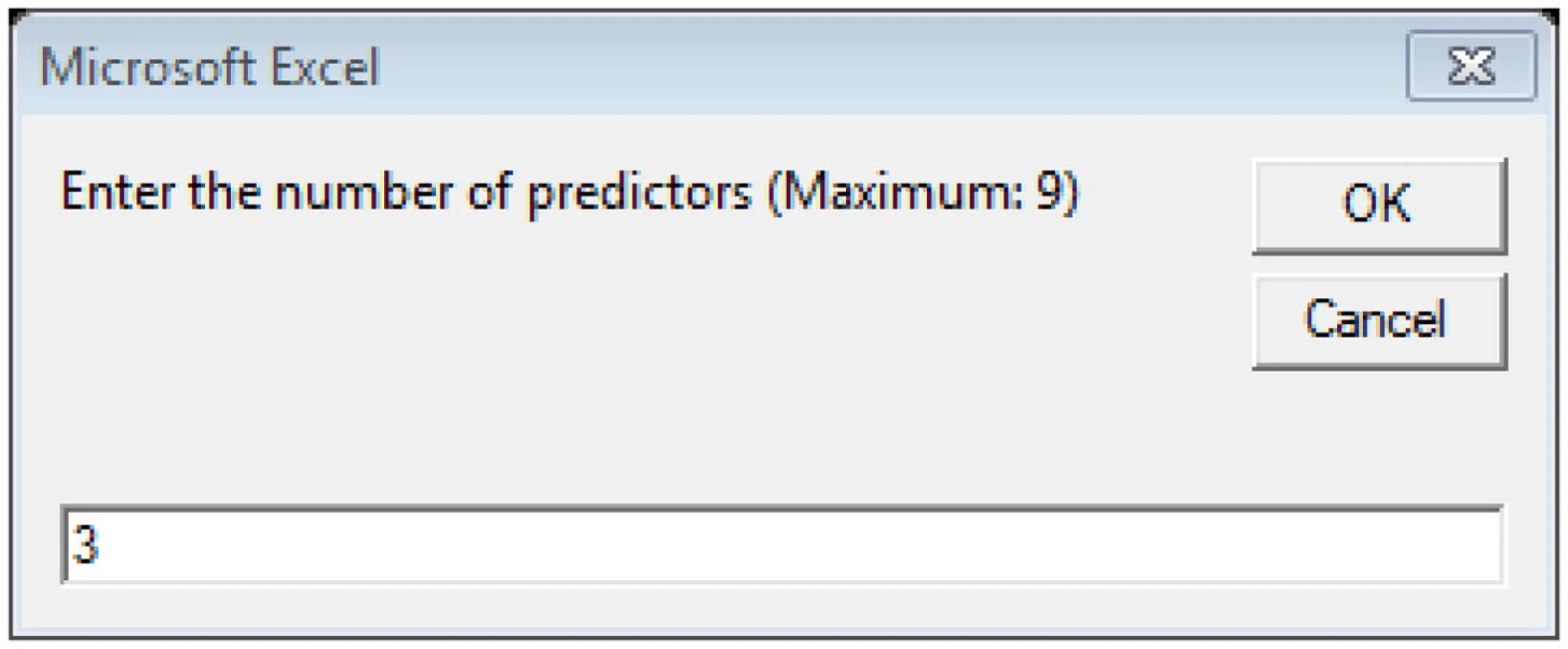
Step 2: Enter the number of predictors and click OK
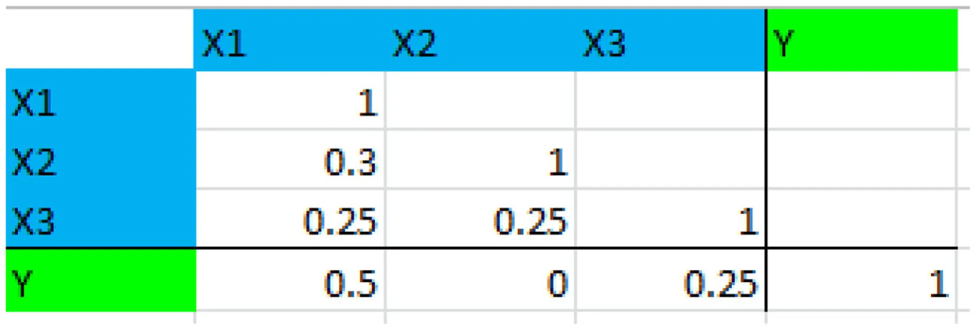
Step 3: Enter the correlation matrix as shown
Step 4: Click Prepare for Analyses to complete the matrix

Step 5: Click Run Analyses

Step 6: Review output in the Results worksheet
R Code for all available analyses
Note. R Code for Versions 2.12.1 and 2.12.2 are demonstrated.
Open R
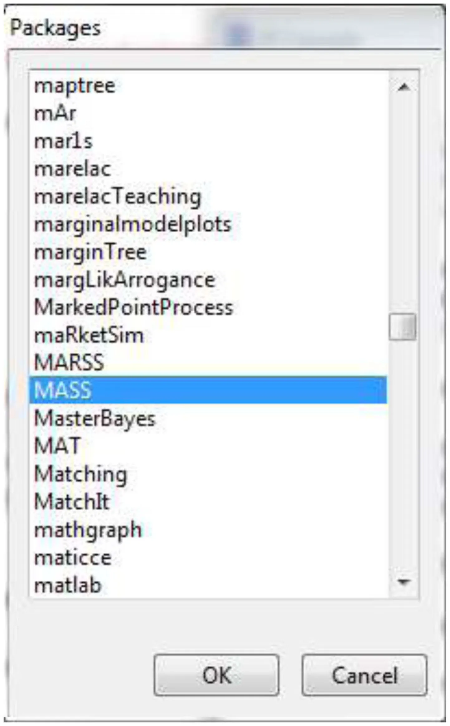
Click on Packages → Install package(s)
Select the one package from a user-selected CRAN mirror site (e.g., USA CA 1)
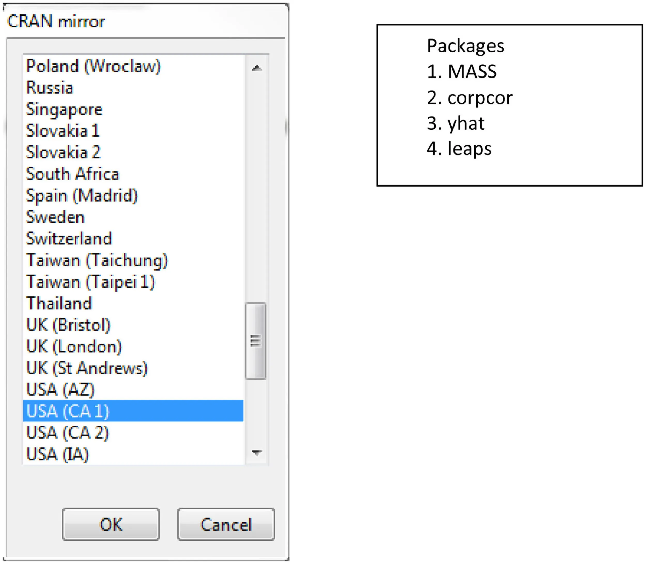
Repeat installation for all four packages
Click on Packages → Load for each package (for a total of four times)
Step 1: Copy and paste the following code to Generate Data from Correlation Matrix
library(MASS)
library(corpcor)
covm<-c(1.00,0.5,0.00,0.25,
0.5, 1,0.3,0.25,
0.0,0.30, 1,0.25,
0.25,0.25,0.25, 1)
covm<-matrix(covm,4,4)
covm<-make.positive.definite(covm)
varlist<-c("DV", "IV1", "IV2", "IV3")
dimnames(covm)<-list(varlist,varlist)
data1<-mvrnorm(n=200,rep(0,4),covm,empirical=TRUE)
data1<-data.frame(data1)
Step 2: Copy and paste the following code to Produce Beta Weights, Structure Coefficients, and Commonality Coefficients
library(yhat)
lmOut<-lm(DV~IV1+IV2+IV3,data1)
regrOut<-regr(lmOut)
regrOut$Beta_Weights
regrOut$Structure_Coefficients
regrOut$Commonality_Data
Step 3: All Possible Subset Analysis
library(leaps)
a<-regsubsets(data1[,(2:4)],data1[,1],method='exhaustive',nbest=7)
cbind(summary(a)$which,rsq = summary(a)$rsq)
SAS code for all available analyses
Note. SAS code is demonstrated in SAS version 9.2.
Open SAS
Click on File → New Program
Step 1: Copy and paste the following code to Generate Data from Correlation Matrix
options pageno = min nodate formdlim = '-';
DATA corr (TYPE=CORR);
LENGTH _NAME_ $ 2;
INPUT _TYPE_ $ _NAME_ $ Y X1 X2 X3;
CARDS;
corr Y 1.00 .500 .000 .250
corr X1 .500 1.00 .300 .250
corr X2 .000 .300 1.00 .250
corr X3 .250 .250 .250 1.00
;
Step 2: Download a SAS macro from UCLA (n.d.) Statistics http://www.ats.ucla.edu/stat/sas/macros/corr2data.sas and save the file as “Corr2Data.sas” to a working directory such as “My Documents”
Step 3: Copy and paste the code below.
%include 'C:\My Documents\corr2data.sas';
%corr2datamycorr, corr, 200, FULL = 'T', corr = 'T');
Step 4: Copy and paste the code below to rename variables with the macro (referenced from http://www.ats.ucla.edu/stat/sas/code/renaming_variables_dynamically.htm)
%macro rename1(oldvarlist, newvarlist);
%let k = 1;
%let old = %scan(&oldvarlist, &k);
%let new = %scan(&newvarlist, &k);
%do %while(("&old" NE "") & ("&new" NE ""));
rename &old = &new;
%let k = %eval(&k + 1);
%let old = %scan(&oldvarlist, &k);
%let new = %scan(&newvarlist, &k);
%end;
%mend;
COMMENT set dataset;
data Azen;
set mycorr;
COMMENT set (old, new) variable names;
%rename1(col1 col2 col3 col4, Y X1 X2 X3);
run;
Step 5: Copy and paste the code below to Conduct Regression Analyses and Produce Beta Weights and Structure Coefficients.
proc reg data=azen; model Y =X1 X2 X3;
output r=resid p=pred;
run;
COMMENT structure coefficients;
proc corr; VAR pred X1 X2 X3;
run;
Step 6: Copy and paste the code below to conduct an All Possible Subset Analysis
proc rsquare; MODEL Y = X1 X2 X3;
run;
Step 7: Link to https://pantherfile.uwm.edu/azen/www/DAonly.txt (Azen and Budescu, 1993)
Step 8: Copy and paste the text below the line of asterisks (i.e., the code beginning at run; option nosource;).
Step 9: Save the SAS file as “dom.sas” to a working directory such as “My Documents.”
Step 8: Copy and paste the code below to conduct a full Dominance Analysis
%include 'C:\My Documents\dom.sas'; *** CHANGE TO PATH WHERE MACRO IS SAVED ***;
%dom(p = 3);
SPSS code for all analyses
Notes. SPSS Code demonstrated in Version 19.0. SPSS must be at least a graduate pack with syntax capabilities.
Reprint Courtesy of International Business Machines Corporation, *(2010) International Business Machines Corporation. The syntax was retrieved from https://www-304.ibm.com/support/docview.wss?uid = swg21480900.
Open SPSS
If a dialog box appears, click Cancel and open SPSS data window.
Click on File → New → Syntax
Step 1: Generate Data from Correlation Matrix. Be sure to specify a valid place to save the correlation matrix. Copy and paste syntax below into the SPSS syntax editor.
matrix data variables= v1 to v4
/contents=corr.
begin data.
1.000
0.500 1.000
0.000 .300 1.000
0.250 .250 .250 1.000
end data.
save outfile="C:\My Documents\corrmat.sav"
/keep=v1 to v4.
Step 2: Generate raw data. Change #i from 200 to your desired N. Change x(4) and #j from 4 to the size of your correlation matrix, if different. Double Check the filenames and locations.
new file.
input program.
loop #i=1 to 200.
vector x(4).
loop #j=1 to 4.
compute x(#j)=rv.normal(0,1).
end loop.
end case.
end loop.
end file.
end input program.
execute.
factor var=x1 to x4
/criteria=factors(4)
/save=reg(all z).
matrix.
get z/var=z1 to z4.
get r/file='C:\My Documents\corrmat.sav'.
compute out=z*chol(r).
save out/outfile='C:\My Documents\AzenData.sav'.
end matrix.
Step 3: Retrieve file generated from the syntax above. Copy and paste the syntax below Highlight the syntax and run the selection by clicking on the
 button.
get file = 'C:\My Documents\AzenData.sav'.
Step 4: Rename variables if desired. Replace “var1 to var10” with appropriate variable names. Copy and paste the syntax below and run the selection by highlighting one line. Be sure to save changes.
rename variables(col1 col2 col3 col4=Y X1 X2 X3).
Step 5: Copy and paste the syntax into the syntax editor to confirm correlations are correct.
CORRELATIONS
/VARIABLES = Y X1 X2 X3
/PRINT = TWOTAIL NOSIG
/MISSING = PAIRWISE.
Step 6: Copy and paste the syntax into the syntax editor to Conduct Regression and Produce Beta Weights.
REGRESSION
/MISSING LISTWISE
/STATISTICS COEFF OUTS R ANOVA
/CRITERIA = PIN(0.05) POUT(0.10)
/NOORIGIN
/DEPENDENT Y
/METHOD = ENTER X1 X2 X3
/SAVE PRED.
Step 7: Copy and paste the syntax into the syntax editor to *Compute Structure Coefficients.
CORRELATIONS
/VARIABLES=X1 X2 X3 WITH PRE_1
/PRINT = TWOTAIL NOSIG
/MISSING = PAIRWISE.
Step 8: All Subset Analysis and Commonality analysis (step 8 to step 11). Before executing, download cc.sps (commonality coefficients macro) from http://profnimon.com/CommonalityCoefficients.sps to working directory such as My Documents.
Step 9: Copy data file to working directory (e.g., C:\My Documents)
Step 10: Copy and paste syntax below in the SPSS syntax editor
CD "C:\My Documents".
INCLUDE FILE="CommonalityCoefficients.sps".
!cc dep = Y
Db=AzenData.sav
Set=Azen
Ind=X1 X2 X3.
Step 11: Retrieve commonality results. Commonality files are written to AzenCommonalityMatrix.sav and AzenCCByVariable.sav. APS files are written toAzenaps.sav.
Step 12: Relative Weights (Step 13 to Step 16).
Step 13: Before executing, download mimr_raw.sps and save to working directory from http://www.springerlink.com/content/06112u8804155th6/supplementals/
Step 14: Open or activate the AzenData.sav dataset file, by clicking on it.
Step 15: If applicable, change the reliabilities of the predictor variables as indicated (4 in the given example).
Step 16: Highlight all the syntax and run; these steps will yield relative importance weights.
Summary
Keywords
multicollinearity, multiple regression
Citation
Kraha A, Turner H, Nimon K, Zientek LR and Henson RK (2012) Tools to Support Interpreting Multiple Regression in the Face of Multicollinearity. Front. Psychology 3:44. doi: 10.3389/fpsyg.2012.00044
Received
21 December 2011
Accepted
07 February 2012
Published
14 March 2012
Volume
3 - 2012
Edited by
Jason W Osborne, Old Dominion University, USA
Reviewed by
Elizabeth Stone, Educational Testing Service, USA; James Stamey, Baylor University, USA
Copyright
© 2012 Kraha, Turner, Nimon, Zientek and Henson.
This is an open-access article distributed under the terms of the Creative Commons Attribution Non Commercial License, which permits non-commercial use, distribution, and reproduction in other forums, provided the original authors and source are credited.
*Correspondence: Amanda Kraha, Department of Psychology, University of North Texas, 1155 Union Circle No. 311280, Denton, TX 76203, USA. e-mail: amandakraha@my.unt.edu
This article was submitted to Frontiers in Quantitative Psychology and Measurement, a specialty of Frontiers in Psychology.
Disclaimer
All claims expressed in this article are solely those of the authors and do not necessarily represent those of their affiliated organizations, or those of the publisher, the editors and the reviewers. Any product that may be evaluated in this article or claim that may be made by its manufacturer is not guaranteed or endorsed by the publisher.